MPP–2006-83
TUM–HEP–638/06
hep–ph/0607103
Low and High Energy Phenomenology of Quark-Lepton Complementarity Scenarios

Abstract

We conduct a detailed analysis of the phenomenology of two predictive see-saw scenarios leading to Quark-Lepton Complementarity. In both cases we discuss the neutrino mixing observables and their correlations, neutrinoless double beta decay and lepton flavor violating decays such as $\mu\rightarrow e\gamma$. We also comment on leptogenesis. The first scenario is disfavored on the level of one to two standard deviations, in particular due to its prediction for $|U_{e3}|$. There can be resonant leptogenesis with quasi-degenerate heavy and light neutrinos, which would imply sizable cancellations in neutrinoless double beta decay. The decays $\mu\rightarrow e\gamma$ and $\tau\rightarrow\mu\gamma$ are typically observable unless the SUSY masses approach the TeV scale. In the second scenario leptogenesis is impossible. It is however in perfect agreement with all oscillation data. The prediction for $\mu\rightarrow e\gamma$ is in general too large, unless the SUSY masses are in the range of several TeV. In this case $\tau\rightarrow e\gamma$ and $\tau\rightarrow\mu\gamma$ are unobservable.

1 Introduction

The neutrino mass and mixing phenomena [1] have provided us with some exciting hints towards the structure of the underlying theory of flavor. In particular, based on observations implying that the CKM and PMNS matrices are linked by a profound connection, an interesting class of models arises. The CKM matrix is to zeroth order the unit matrix plus a small correction, given by the sine of the Cabibbo angle, $\sin\theta_{C}=0.23$. Hence, in the quark sector mixing is absent at zeroth order and the deviation from no mixing is small. To make a connection to the lepton sector, it was noted [2] that the deviation from maximal mixing is small. Indeed, using the bimaximal [3] mixing scenario as the zeroth order scheme and interpreting the observed deviation from maximal solar neutrino mixing as a small expansion parameter, one can write [2]:

$$|U_{e2}|\equiv\sqrt{\frac{1}{2}}\,\left(1-\lambda_{\nu}\right)~{}.$$ (1)

With current experimental information [4], we obtain $\lambda_{\nu}=0.21^{+0.04,\,0.08,\,0.11}_{-0.03,\,0.07,\,0.11}$, where we have inserted the best-fit values and the 1, 2 and $3\sigma$ ranges of the relevant oscillation parameters. This number is remarkably similar to the Cabibbo angle [2]. In fact, the so called QLC-relation (Quark-Lepton Complementarity) [5, 6]

$$\theta_{12}+\theta_{C}=\frac{\pi}{4}~{}$$ (2)

has been suggested and several situations in which it can be realized have been discussed [5, 6, 7, 8, 9]. In general, the PMNS matrix is given by $U_{\ell}^{\dagger}\,U_{\nu}$, where $U_{\nu}$ diagonalizes the neutrino mass matrix and $U_{\ell}$ originates from the charged lepton diagonalization. Apparently, deviations from maximal $\theta_{12}$ as implied by Eqs. (1, 2) can be obtained if the neutrino mass matrix corresponds to bimaximal mixing and the charged lepton mass matrix is diagonalized by either the CKM or a CKM-like [10, 11] matrix. The opposite case, namely bimaximal mixing from the charged lepton sector and a CKM correction from the neutrinos, can also be realized, which indicates two possibilities for the approximate realization of Eq. (2).

In the present article we fully analyze the phenomenology of these two popular scenarios, proposed in [5, 6], leading to an approximate realization of QLC within the see-saw mechanism [12]. The two scenarios show the feature that the matrix perturbing the bimaximal mixing scenario is exactly the CKM matrix and not just a CKM-like matrix, which minimizes the number of free parameters. We study the neutrino oscillation phenomenology, neutrinoless double beta decay and – in context of the see-saw mechanism – lepton flavor violating decays such as $\mu\to e\gamma$. We present our results of the correlations between the observables in several plots. In contrast to many previous works, we include the full number of possible $CP$ phases. This is a new approach particularly for the second scenario, where bimaximal mixing arises from the charged lepton sector. For both scenarios we comment on the prospects of leptogenesis. We begin in Sec. 2 with an introduction to the formalism required to study the observables. In Secs. 3 and 4 we discuss the phenomenology of the two scenarios, before we conclude in Sec. 5 with a summary of our results.

2 Formalism

In this section we briefly introduce the required formalism to analyze the QLC scenarios. First, we discuss lepton and quark mixing before turning to lepton flavor violation, whose connection to low energy neutrino physics is implied by the see-saw mechanism. Conclusively, the principles of leptogenesis are outlined.

2.1 Neutrino Masses, Lepton- and Quark-Mixing

The two scenarios leading to QLC are set within the framework of the see-saw mechanism for neutrino mass generation [12]. In general, one has the Lagrangian

$${\cal L}=\frac{1}{2}\,\overline{N_{R}}\,M_{R}\,N_{R}^{c}+\overline{\ell_{R}}\,m_{\ell}\,\ell_{L}+\overline{N_{R}}\,m_{D}\,\nu_{L}~{},$$ (3)

where $N_{R}$ are the right-handed Majorana singlets, $\ell_{L,R}$ the left- and right-handed charged leptons and $\nu_{L}$ the left-handed neutrinos. The mass matrix of the charged leptons is $m_{\ell}$, $m_{D}$ is the Dirac neutrino mass matrix and $M_{R}$ the heavy right-handed Majorana neutrino mass matrix. As $M_{R}\gg m_{D}$, Eq. (3) leads to an effective neutrino mass matrix at low energies, defined as

$$m_{\nu}=-m_{D}^{T}\,M_{R}^{-1}\,m_{D}=U_{\nu}^{\ast}\,m_{\nu}^{\rm diag}\,U_{\nu}^{\dagger}~{},$$ (4)

where $U_{\nu}$ transforms $m_{\nu}$ to $m_{\nu}^{\rm diag}$, with the neutrino masses $m_{1,2,3}$ as diagonal entries. When diagonalizing the charged lepton mass matrix as $m_{\ell}=V_{\ell}\,m_{\ell}^{\rm diag}\,U_{\ell}^{\dagger}$, we can rotate $\nu_{L}\rightarrow U_{\nu}^{\dagger}\,\nu_{L}$, $\ell_{R}\rightarrow V_{\ell}^{\dagger}\,\ell_{R}$ and $\ell_{L}\rightarrow U_{\ell}^{\dagger}\,\ell_{L}$. From the charged current term, which is proportional to $\overline{\ell_{L}}\,\gamma^{\mu}\,\nu_{L}$, we thus obtain the PMNS matrix

$$U=U_{\ell}^{\dagger}\,U_{\nu}~{},$$ (5)

which we parameterize as

$$U=\left(\begin{array}[]{ccc}c_{12}c_{13}&s_{12}c_{13}&s_{13}\,e^{-i\delta}\\[5.69046pt] -s_{12}c_{23}-c_{12}s_{23}s_{13}e^{i\delta}&c_{12}c_{23}-s_{12}s_{23}s_{13}e^{i\delta}&s_{23}c_{13}\\[5.69046pt] s_{12}s_{23}-c_{12}c_{23}s_{13}e^{i\delta}&-c_{12}s_{23}-s_{12}c_{23}s_{13}e^{i\delta}&c_{23}c_{13}\\ \end{array}\right){\rm diag}(1,e^{i\alpha},e^{i(\beta+\delta)})\,,$$ (6)

where we have used the usual notations $c_{ij}=\cos\theta_{ij}$, $s_{ij}=\sin\theta_{ij}$. We have also introduced the Dirac $CP$-violating phase $\delta$ and the two Majorana $CP$-violating phases $\alpha$ and $\beta$ [13]. The oscillation parameters can be expressed by two independent mass squared differences, $\mbox{$\Delta m^{2}_{\odot}$}=m_{2}^{2}-m_{1}^{2}$ and $\mbox{$\Delta m^{2}_{\rm A}$}=|m_{3}^{2}-m_{1}^{2}|$, as well as three mixing angles, whose exact values are a matter of intense research projects [1]. Their current best-fit values and their 1, 2 and 3$\sigma$ ranges are according to Ref. [4]:

$$\Delta m^{2}_{\odot} = \left(7.9^{+0.3,\,0.6,\,1.0}_{-0.3,\,0.6,\,0.8}\right)\cdot 10^{-5}\mbox{ eV}^{2}~{},$$

$$\sin^{2}\theta_{12} = 0.31^{+0.02,\,0.06,\,0.09}_{-0.03,\,0.05,\,\,0.07}~{},$$

$$\Delta m^{2}_{\rm A} = \left(2.2^{+0.37,\,0.7,\,1.1}_{-0.27,\,0.5,\,0.8}\right)\cdot 10^{-3}\mbox{ eV}^{2}~{},$$ (7)

$$\sin^{2}\theta_{23} = 0.50^{+0.06,\,0.14,\,0.18}_{-0.05,\,0.12,\,0.16}~{},$$

$$\sin^{2}\theta_{13} < 0.012~{}(0.028,\,0.046)~{}.$$

The present best-fit value for $\sin^{2}\theta_{13}$ is 0 and there is no information on any of the phases.

Turning to the quark sector, the CKM matrix is [14]

$$V=\left(\begin{array}[]{ccc}1-\frac{1}{2}\,\lambda^{2}&\lambda&A\,\lambda^{3}\,(\rho-i\eta)\\[8.5359pt] -\lambda&1-\frac{1}{2}\,\lambda^{2}&A\,\lambda^{2}\\[8.5359pt] A\,\lambda^{3}\,(1-\rho+i\eta)&-A\,\lambda^{2}&1\end{array}\right)+{\cal{O}}(\lambda^{4})~{}.$$ (8)

In analogy to the PMNS matrix it is a product of two unitary matrices, $V=V_{\rm up}^{\dagger}\,V_{\rm down}$, where $V_{\rm up}$ ($V_{\rm down}$) is associated with the diagonalization of the up-(down-)quark mass matrix. As reported in [15] the best-fit values as well as the 1, 2 and 3$\sigma$ ranges of the parameters $\lambda,A,\bar{\rho},\bar{\eta}$ are

$$\begin{array}[]{c}\lambda=\sin\theta_{C}=0.2272^{+0.0010,\,0.0020,\,0.0030}_{-0.0010,\,0.0020,\,0.0030}~{},\\[5.69046pt] A=0.809^{+0.014,\,0.029,\,0.044}_{-0.014,\,0.028,\,0.042}~{},\\[5.69046pt] \bar{\rho}=0.197^{+0.026,\,0.050,\,0.074}_{-0.030,\,0.087,\,0.133}~{},\\[5.69046pt] \bar{\eta}=0.339^{+0.019,\,0.047,\,0.075}_{-0.018,\,0.037,\,0.057}~{},\end{array}$$ (9)

where $\bar{\rho}=\rho\,(1-\lambda^{2}/2)$ and $\bar{\eta}=\eta\,(1-\lambda^{2}/2)$. Effects caused by $CP$ violation are always proportional to a Jarlskog invariant [16], defined as

$$J_{CP}=-{\rm Im}\{V_{ud}\,V_{cs}\,V_{us}^{\ast}\,V_{cd}^{\ast}\}\simeq A^{2}\,\lambda^{6}\,\bar{\eta}=\left(3.1^{+0.43,\,0.82,\,1.08}_{-0.37,\,0.74,\,0.96}\right)\cdot 10^{-5}~{}.$$ (10)

The leptonic analogue of Eq. (10) is

$$J_{CP}^{\rm lep}={\rm Im}\left\{U_{e1}\,U_{\mu 2}\,U_{e2}^{\ast}\,U_{\mu 1}^{\ast}\right\}=\frac{1}{8}\,\sin 2\theta_{12}\,\sin 2\theta_{23}\,\sin 2\theta_{13}\,\cos\theta_{13}\,\sin\delta~{},$$ (11)

where we have also given the explicit form of $J_{CP}^{\rm lep}$ with the parameterization of Eq. (6). There are two additional invariants, $S_{1}$ and $S_{2}$ [17], related to the Majorana phases:

$$\begin{array}[]{c}S_{1}={\rm Im}\left\{U_{e1}\,U_{e3}^{\ast}\right\}\mbox{ and }S_{2}={\rm Im}\left\{U_{e2}\,U_{e3}^{\ast}\right\}~{},\end{array}$$ (12)

which have no analogue in the quark sector.

2.2 Lepton Flavor Violation

The see-saw mechanism explains the smallness of neutrino masses, but due to the extreme heaviness of the right-handed Majorana neutrinos a direct test is not only challenging, but presumably impossible. Nonetheless a reconstruction of the see-saw parameter space is possible in supersymmetric (SUSY) scenarios. While being extremely suppressed when mediated by light neutrinos [18], Lepton Flavor Violating (LFV) decays such as $\mu\rightarrow e\gamma$ depend in the context of SUSY see-saw on the very same parameters responsible for neutrino masses and can be observable in this case [19]. The size and relative magnitudes of the decays are known to be a useful tool to distinguish between different models. In this work we will focus on models where SUSY is broken by gravity mediation, so called mSUGRA models. In this case there are four relevant parameters, which are defined at the GUT scale $M_{X}$, namely the universal scalar mass $m_{0}$, the universal gaugino mass $m_{1/2}$, the universal trilinear coupling parameter $A_{0}$ and $\tan\beta$, which is the ratio of the vacuum expectation values of the up- and down-like Higgs doublets. For the branching ratios of the decays $\mu\rightarrow e\gamma$, $\tau\rightarrow e\gamma$ and $\tau\rightarrow\mu\gamma$ one can obtain in the leading-log approximation [19]

$$\text{BR}(l_{i}\to l_{j}\gamma)\simeq\frac{\Gamma(l_{i}\to e\nu\bar{\nu})}{\Gamma_{\text{total}}(l_{i})}\frac{\alpha_{\text{em}}^{3}}{G_{F}^{2}\,m_{S}^{8}\,v_{u}^{4}}\left(\frac{3m_{0}^{2}+A_{0}^{2}}{8\pi^{2}}\right)^{2}\left|\left(\tilde{m}_{D}^{\dagger}\,L\,\tilde{m}_{D}\right)_{ij}\right|^{2}\,\tan^{2}\beta\;.$$ (13)

Here $v_{u}=v\,\sin\beta$ with $v=174$ GeV, $m_{S}$ represents a SUSY particle mass and $L=\delta_{ij}\ln M_{X}/M_{i}$, with $M_{i}$ the heavy Majorana masses and $M_{X}=2\cdot 10^{16}$ GeV. Note that the formulae relevant for lepton flavor violation and leptogenesis have to be evaluated in the basis in which the charged leptons and the heavy Majorana neutrinos are real and diagonal. In this very basis we have to replace

$$m_{D}\rightarrow\tilde{m}_{D}=V_{R}^{T}\,m_{D}\,U_{\ell}~{},$$ (14)

where $V_{R}$ diagonalizes the heavy Majorana mass matrix via $M_{R}=V_{R}^{\ast}\,M_{R}^{\rm diag}\,V_{R}^{\dagger}$. The current limit on the branching ratio of $\mu\to e\gamma$ is $1.2\cdot 10^{-11}$ at 90% C.L. [20]. A future improvement of two orders of magnitude is expected [21]. In most parts of the relevant soft SUSY breaking parameter space, the expression

$$m_{S}^{8}\simeq 0.5~{}m_{0}^{2}~{}m_{1/2}^{2}~{}(m_{0}^{2}+0.6~{}m_{1/2}^{2})^{2}\;,$$ (15)

is an excellent approximation to the results obtained in a full renormalization group analysis [22]. In order to simplify comparisons of different scenarios, it can be convenient to use “benchmark values” of the SUSY parameters. We choose both pints and slopes of the SPS values [23] displayed in Table 1.

Point	$m_{0}$	$m_{1/2}$	$A_{0}$	$\tan\beta$
1a	100	250	$-100$	10
1b	200	400	0	30
2	1450	300	0	10
3	90	400	0	10
4	400	300	0	50

Table 1: SPS Benchmark values for the mSUGRA parameters according to Ref. [23]. The values of $m_{0}$, $m_{1/2}$ and $A_{0}$ are in GeV. The slope for Point 1a (2, 3) is $m_{0}=-A_{0}=0.4\,m_{1/2}$ ($m_{0}=2\,m_{1/2}+850$ GeV, $m_{0}=\frac{1}{4}\,m_{1/2}-10$ GeV) with varying $m_{1/2}$.

In this context it might be worth commenting on renormalization aspects of the QLC relation (see also [6]). The running of the CKM parameters can always be neglected. However, the case of a large $\tan\beta\mathrel{\hbox to0.0pt{\raise 2.20013pt\hbox{$>$}\hss}{\lower 2.20013pt\hbox{$\sim$}}}10$ in the MSSM can imprint sizeable effects on the neutrino observables, if the neutrino masses are not normally ordered. In our analysis, this would affect only the SPS point 4, when the neutrinos have an inverted hierarchy or are quasi-degenerate.

It proves useful to consider also the “double” ratios,

$$\begin{array}[]{c}R(21/31)\displaystyle\equiv\frac{\text{BR}(\mu\to e+\gamma)}{\text{BR}(\tau\to e+\gamma)}\simeq\frac{\left|(\tilde{m}_{D}^{\dagger}\,L\,\tilde{m}_{D})_{21}\right|^{2}}{\left|(\tilde{m}_{D}^{\dagger}\,L\,\tilde{m}_{D})_{31}\right|^{2}}\;,\\[8.5359pt] R(21/32)\displaystyle\equiv\frac{\text{BR}(\mu\to e+\gamma)}{\text{BR}(\tau\to\mu+\gamma)}\simeq\frac{\left|(\tilde{m}_{D}^{\dagger}\,L\,\tilde{m}_{D})_{21}\right|^{2}}{\left|(\tilde{m}_{D}^{\dagger}\,L\,\tilde{m}_{D})_{32}\right|^{2}}\;,\end{array}$$ (16)

which are essentially independent of the SUSY parameters.

2.3 Leptogenesis

Since we will also comment on the possibility of leptogenesis in the QLC scenarios, we will summarize the key principles of this mechanism. An important challenge in modern cosmology is the explanation of the baryon asymmetry $\eta_{B}\simeq 6\cdot 10^{-10}$ [25] of the Universe. One of the most popular mechanisms to create the baryon asymmetry is leptogenesis [26]. The heavy neutrinos, whose comparatively huge masses govern the smallness of the light neutrino masses, decay in the early Universe into Higgs bosons and leptons, thereby generating a lepton asymmetry, which in turn gets recycled into a baryon asymmetry via non-perturbative Standard Model processes. For recent reviews, see [27]. In principle, all three heavy neutrinos generate a decay asymmetry, which can be written as (summed over all flavors)

$$\begin{array}[]{c}\varepsilon_{i}\displaystyle=\frac{1}{8\pi\,v_{u}^{2}}\,\frac{1}{\left(\tilde{m}_{D}\,\tilde{m}_{D}^{\dagger}\right)_{ii}}\,\sum\limits_{j\neq i}{\rm Im}\left\{\left(\tilde{m}_{D}\,\tilde{m}_{D}^{\dagger}\right)_{ji}^{2}\right\}\,\sqrt{x_{j}}\,\left(\frac{2}{1-x_{j}}-\ln\left(\frac{1+x_{j}}{x_{j}}\right)\right)~{},\\[8.5359pt] \displaystyle\varepsilon_{1}\simeq-\frac{3}{8\pi\,v_{u}^{2}}\,\frac{1}{\left(\tilde{m}_{D}\,\tilde{m}_{D}^{\dagger}\right)_{11}}\,\sum\limits_{j=2,3}\,{\rm Im}\left\{\left(\tilde{m}_{D}\,\tilde{m}_{D}^{\dagger}\right)_{j1}^{2}\right\}\,\frac{M_{1}}{M_{j}}~{},\end{array}$$ (17)

where $x_{j}=M_{j}^{2}/M_{i}^{2}$. This is the general form of $\varepsilon_{i}$ and the limit for $\varepsilon_{1}$ in case of $M_{3}\gg M_{2}\gg M_{1}$. Note that the decay asymmetries depend on $\tilde{m}_{D}\,\tilde{m}_{D}^{\dagger}$, which has to be compared to the dependence on $\tilde{m}_{D}^{\dagger}\,\tilde{m}_{D}$ governing the LFV decays. In the case $M_{3}\gg M_{2}\gg M_{1}$ only $\varepsilon_{1}$ plays a role, and dedicated numerical studies [27, 28] have shown that in case of the MSSM and a hierarchical spectrum of the heavy Majorana neutrino masses, successful thermal leptogenesis is only possible for

$$m_{1}\mathrel{\hbox to0.0pt{\raise 2.20013pt\hbox{$<$}\hss}{\lower 2.20013pt\hbox{$\sim$}}}0.1~{}{\rm eV}\mbox{ and }M_{1}\mathrel{\hbox to0.0pt{\raise 2.20013pt\hbox{$>$}\hss}{\lower 2.20013pt\hbox{$\sim$}}}10^{9}~{}{\rm GeV}~{}.$$ (18)

However, it can occur in certain models that the lightest heavy neutrino mass is smaller than the limit of $10^{9}$ GeV given above. We will encounter a scenario like this in the next section. There are three possible ways to resolve this problem:

• the decay of the second heaviest neutrino can in certain scenarios generate the baryon asymmetry. Flavor effects [29, 30] are important in this respect;

• if the heavy Majorana neutrinos are quasi-degenerate in mass, the decay asymmetry can be resonantly enhanced, as has been analyzed in [31]. This requires some amount of tuning;

• non-thermal leptogenesis, i.e., the production of heavy neutrinos via inflaton decay [32]. This possibility is a more model dependent case and complicates the situation, as the reheating temperature, the mass of the inflaton and the corresponding branching ratios for its decay into the Majorana neutrinos need to be known.

Let us comment a bit on the first case: the expression for the decay asymmetry Eq. (17) has been obtained by summing over all flavors in which the heavy neutrino decays. Recently, however, is has been realized that flavor effects on leptogenesis can have significant impact on the scenario [29, 30]. The decay asymmetry for the decay of the heavy neutrino in a lepton of flavor $\alpha=e,\mu,\tau$ has to be evaluated individually and the wash-out or distribution for each flavor has to be followed individually by its own Boltzmann-equation. However, the bound on the lightest heavy neutrino mass $M_{1}$ is essentially the same as in the “summed over all flavors” approach. In addition, the decay asymmetry in this approach can be enhanced by at most one order of magnitude. What will be interesting for our purpose is that if $M_{1}\ll 10^{9}$ GeV the second heaviest neutrino with mass $M_{2}$ can in principle generate the baryon asymmetry [30], as long as the wash-out by the lightest heavy neutrino is low. We will discuss this in more detail in Section 3.3.

3 First Realization of QLC

The first framework in which our analysis is set is the following:

• we assume the conventional see-saw mechanism to generate the neutrino mass matrix $m_{\nu}=-m_{D}^{T}\,M_{R}^{-1}\,m_{D}$. Diagonalization of $m_{\nu}$ is achieved via $m_{\nu}=U_{\nu}^{\ast}\,m_{\nu}^{\rm diag}\,U_{\nu}^{\dagger}$ and $U_{\nu}$ produces exact bimaximal mixing;

• the PMNS matrix is given by $U=U_{\ell}^{\dagger}\,U_{\nu}$, where $U_{\ell}$ corresponds to the CKM matrix $V$. This can be achieved in some $SU(5)$ models, in which $m_{\ell}=m_{\rm down}^{T}$, where $m_{\rm down}$ is the down-quark mass matrix. Hence, $V_{\rm down}=V$. Consequently, the up-quark mass matrix $m_{\rm up}$ is real and diagonal;

• in some $SO(10)$ models it holds that $m_{\rm up}=m_{D}$. It follows that the bimaximal structure of $m_{\nu}$ originates from $M_{R}$, which is diagonalized by $M_{R}=V_{R}^{\ast}\,M_{R}^{\rm diag}\,V_{R}^{\dagger}$.

This scenario has been outlined already in [5, 6]. Note that only $U_{\ell}=V$ is required for the low energy realization of QLC and that the relation $m_{\ell}=m_{\rm down}^{T}$ will not be required to calculate the branching ratios of the LFV decays or the baryon asymmetry. It is known that $m_{\ell}=m_{\rm down}^{T}$ is not realistic for the first and second fermion generation. More “realistic” scenarios have been analyzed in Refs. [8, 33], in which the relation $m_{\ell}=m_{\rm down}^{T}$ is modified by the Georgi-Jarlskog factor [34]. However, in this case the neutrinos can not be diagonalized by a bimaximal mixing matrix, because a too large solar neutrino mixing angle would result. Consequently the minimality of the scenarios is lost, and the QLC relation $\theta_{12}+\theta_{C}=\pi/4$ turns out to be just a numerical coincidence. Therefore, following most of the analyzes in Refs. [5, 6, 7], we assume that there is a particular structure on the mass matrices in which mixing depends only weakly on the mass eigenvalues.

With the indicated set of properties, we can express Eq. (5) as

$$U=V^{\dagger}\,U_{\rm bimax}~{},$$ (19)

with $U_{\rm bimax}$ corresponding to bimaximal mixing, which will be precisely defined in Eq. (21). Moreover, Eq. (14) changes to

$$\tilde{m}_{D}=V_{R}^{T}\,m_{D}\,V\Rightarrow\left\{\begin{array}[]{cc}\tilde{m}_{D}^{\dagger}\,\tilde{m}_{D}=V^{\dagger}\,{\rm diag}(m_{u}^{2},m_{c}^{2},m_{t}^{2})\,V&\mbox{ for LFV}~{},\\[8.5359pt] \tilde{m}_{D}\,\tilde{m}_{D}^{\dagger}=V_{R}^{T}\,{\rm diag}(m_{u}^{2},m_{c}^{2},m_{t}^{2})\,V_{R}^{\ast}&\mbox{ for }\eta_{B}~{}.\end{array}\right.$$ (20)

In the above equation we have given the two important matrices $\tilde{m}_{D}\,\tilde{m}_{D}^{\dagger}$ and $\tilde{m}_{D}^{\dagger}\,\tilde{m}_{D}$ describing leptogenesis and the branching ratios of the lepton flavor violating processes. Note however, that for the latter we have for now neglected the logarithmic dependence on the heavy neutrino masses, cf. Eq. (13).

3.1 Low Energy Neutrino Phenomenology

The matrix diagonalizing $m_{\nu}$ is called $U_{\nu}$ and corresponds to a bimaximal mixing matrix:

$$U_{\nu}=U_{\rm bimax}=P_{\nu}\,\tilde{U}_{\rm bimax}\,Q_{\nu}={\rm diag}(1,e^{i\phi},e^{i\omega})\,\left(\begin{array}[]{ccc}\frac{1}{\sqrt{2}}&\frac{1}{\sqrt{2}}&0\\[8.5359pt] -\frac{1}{2}&\frac{1}{2}&\frac{1}{\sqrt{2}}\\[8.5359pt] \frac{1}{2}&-\frac{1}{2}&\frac{1}{\sqrt{2}}\\[8.5359pt] \end{array}\right){\rm diag}(1,e^{i\sigma},e^{i\tau})~{}.$$ (21)

We have included two diagonal phase matrices $P_{\nu}$ and $Q_{\nu}$. It has been shown in Ref. [11] that this is the most general form if all ”unphysical” phases are rotated away. We have in total five phases, one phase in $U_{\ell}=V$ and four phases in $U_{\nu}$. Note that $Q_{\nu}$ is “Majorana-like” [11], i.e., the phases $\sigma$ and $\tau$ do not appear in neutrino oscillations, but contribute to the low energy Majorana phases. Multiplying the matrices of Eq. (8) and Eq. (21) yields for the oscillation parameters:

$$\begin{array}[]{c}U=U_{\ell}^{\dagger}\,U_{\nu}=V^{\dagger}\,U_{\rm bimax}\\[8.5359pt] \Rightarrow\left\{\begin{array}[]{c}\sin^{2}\theta_{12}=\frac{\displaystyle 1}{\displaystyle 2}-\frac{\displaystyle\lambda}{\displaystyle\sqrt{2}}\,\cos\phi+{\cal O}(\lambda^{3})~{},\\[5.69046pt] |U_{e3}|=\frac{\displaystyle\lambda}{\displaystyle\sqrt{2}}+{\cal O}(\lambda^{3})~{},\\[5.69046pt] \sin^{2}\theta_{23}=\frac{\displaystyle 1}{\displaystyle 2}-\left(A\,\cos(\omega-\phi)+\frac{1}{4}\right)\,\lambda^{2}+{\cal O}(\lambda^{4})~{},\\[5.69046pt] J_{CP}^{\rm lep}=\frac{\displaystyle\lambda}{\displaystyle 4\sqrt{2}}\,\sin\phi+{\cal O}(\lambda^{3})~{}.\end{array}\right.\end{array}$$ (22)

Apparently, Eq. (22) generates correlations between the observables. The solar neutrino mixing parameter depends on the $CP$ phase $\phi$, which originates from the neutrino sector and is to a very good approximation the phase governing leptonic $CP$ violation in oscillation experiments. Note that in order to have solar neutrino mixing of the observed magnitude, the phase has to be close to zero or $2\pi$. Approximately, at $3\sigma$ it should be below $\pi/4$ or above $7\pi/4$. The smallest solar neutrino mixing angle is obtained for $\phi=0$ and the prediction for $\sin^{2}\theta_{12}$ is

$$\sin^{2}\theta_{12}\mathrel{\hbox to0.0pt{\raise 2.20013pt\hbox{$>$}\hss}{\lower 2.20013pt\hbox{$\sim$}}}0.334~{}(0.333,\,0.332,\,0.331)~{}.$$ (23)

This value of $\sin^{2}\theta_{12}\mathrel{\hbox to0.0pt{\raise 2.20013pt\hbox{$>$}\hss}{\lower 2.20013pt\hbox{$\sim$}}}0.33$ has to be compared with the experimental $1\sigma$ ($2\sigma$) limit of $\sin^{2}\theta_{12}\leq 0.33~{}(0.37)$, showing a small conflict. Note that for the numerical values, as well as for the generation of the plots, which will be presented and discussed in the following, we did not use the approximate expressions in Eq. (22), but the exact formulae. Besides the phases, we also vary the parameters of the CKM matrix in their 1, 2 and 3$\sigma$ ranges (though in particular the error in $\lambda$ is negligible), and also fix these parameters to their best-fit values. Even for the best-fit values of the CKM parameters, there results a range of values, which is caused by the presence of the unknown phases $\phi$ and $\omega$. To a good approximation, $|U_{e3}|$ is the sine of the Cabibbo angle divided by $\sqrt{2}$, leading to a sharp prediction of $|U_{e3}|^{2}=0.0258$. Varying the phases and the CKM parameters, we find a range of

$$|U_{e3}|=0.1607^{+0.0058,\,0.0069,\,0.0083,\,0.0096}_{-0.0059,\,0.0068,\,0.0080,\,0.0091}~{},$$ (24)

where we took the central value $\lambda/\sqrt{2}=0.1607$. Recall that the $1\sigma$ ($2\sigma$) bound on $|U_{e3}|$ is 0.11 (0.17). Therefore, the prediction for $|U_{e3}|$ is incompatible with the current 1$\sigma$ bound of $|U_{e3}|$ and even quite close to the $2\sigma$ limit. The experiments taking data in the next 5 to 10 years [35] will have to find a signal corresponding to non-vanishing $|U_{e3}|$ in order for this particular framework to survive. Leptonic $CP$ violation is in leading order proportional to $\lambda\,\sin\phi$, which is five orders in units of $\lambda$ larger than the $J_{CP}$ of the quark sector. If the neutrino sector conserved $CP$, one would obtain $J_{CP}^{\rm lep}=\frac{1}{8}\,A\,\eta\,\lambda^{4}$, which is still two orders of $\lambda$ larger than the $J_{CP}$ of the quark sector. If $V$ was equal to the unit matrix, which corresponds to bimaximal mixing in the PMNS matrix, $J_{CP}^{\rm lep}$ would be zero. There is an interesting “sum-rule” between leptonic $CP$ violation, solar neutrino mixing and $|U_{e3}|$:

$$\begin{array}[]{c}\sin^{2}\theta_{12}\simeq\frac{1}{2}-|U_{e3}|\,\cos\phi\simeq\frac{1}{2}\pm\sqrt{|U_{e3}|^{2}-16\,(J_{CP}^{\rm lep})^{2}}~{}.\end{array}$$ (25)

Overall, the experimental result of $\sin^{2}\theta_{12}\simeq 0.31$ implies large $\cos\phi$, and therefore small $\sin\phi$, leading to small $CP$ violating effects even though $|U_{e3}|$ is sizable. Atmospheric neutrino mixing stays very close to maximal and due to cancellations $\sin^{2}\theta_{23}=\frac{1}{2}$ can always occur. If $\cos(\omega-\phi)=1$, then $\sin^{2}\theta_{23}$ takes its minimal value. We have seen above that the observed low value of the solar neutrino mixing angle requires $\phi\simeq 0$, so that $\omega\simeq 0$ is implied when $\theta_{23}$ is very close to maximal. The minimal and maximal values of $\sin^{2}\theta_{23}$ are given by

$$\sin^{2}\theta_{23}\geq 0.445~{}(0.444,\,0.443,\,0.442)~{}\mbox{ and }\sin^{2}\theta_{23}\leq 0.531~{}(0.532,\,0.533,\,0.534)~{}.$$ (26)

Probing deviations from maximal mixing of order 10% could be possible in future experiments [35]. In Fig. 1 we show the correlations between the oscillation parameters which result from the relation $U=V^{\dagger}\,U_{\rm bimax}$ in Eq. (22). We plot $J_{CP}^{\rm lep}$, $\phi$ and $\sin^{2}\theta_{23}$ against $\sin^{2}\theta_{12}$, as well as $\sin^{2}\theta_{23}$ against $|U_{e3}|$. We also indicate the current 1, 2 and $3\sigma$ ranges of the oscillation parameters. This shows again that solar neutrino mixing is predicted to be close to its 1$\sigma$ bound and $|U_{e3}|$ even close to its 2$\sigma$ bound.

Now we turn to the neutrino observables outside the oscillation framework and comment on the consequences for neutrinoless double beta decay. The two invariants related to the Majorana phases are

$$\begin{array}[]{c}S_{1}=\frac{\displaystyle\lambda}{\displaystyle 2}\,\sin(\phi+\tau)+\frac{\displaystyle\lambda^{2}}{\displaystyle 2\sqrt{2}}\,\sin\tau+{\cal O}(\lambda^{3})~{},\\[8.5359pt] S_{2}=\frac{\displaystyle\lambda}{\displaystyle 2}\,\sin(\phi-\sigma+\tau)+\frac{\displaystyle\lambda^{2}}{\displaystyle 2\sqrt{2}}\,\sin(\sigma-\tau)+{\cal O}(\lambda^{3})~{}.\end{array}$$ (27)

As expected, the two phases $\sigma$ and $\tau$ in $Q_{\nu}$ only appear in these quantities. According to the parameterization of Eq. (6), we have $S_{1}=-c_{12}\,c_{13}\,s_{13}\,s_{\beta}$ and $S_{2}=s_{12}\,c_{13}\,s_{13}\,s_{\alpha-\beta}$. We can insert in Eq. (27) the expressions for the mixing angles from Eq. (22) to obtain in leading order $\sin\beta\simeq-\sin(\phi+\tau)$ and $\sin(\alpha-\beta)\simeq\sin(\phi-\sigma+\tau)$. Hence, the Majorana phase $\sigma$ is related to the phase $\alpha$ in the parameterization of Eq. (6). It is interesting to study the form of the neutrino mass matrix, which is responsible for bimaximal mixing. It reads

$$\begin{array}[]{c}m_{\nu}^{\rm bimax}=\left(\begin{array}[]{ccc}\displaystyle A&B\,e^{-i\phi}&-B\,e^{-i\omega}\\[5.69046pt] \displaystyle\cdot&(D+\frac{A}{2})\,e^{-2i\phi}&(D-\frac{A}{2})\,e^{-i(\phi+\omega)}\\[8.5359pt] \displaystyle\cdot&\cdot&(D+\frac{A}{2})\,e^{-2i\omega}\end{array}\right)\\[8.5359pt] =\left(\begin{array}[]{ccc}1&0&0\\[5.69046pt] 0&e^{-i\phi}&0\\[5.69046pt] 0&0&e^{-i\omega}\end{array}\right)\left(\begin{array}[]{ccc}\displaystyle A&B&-B\\[5.69046pt] \displaystyle\cdot&D+\frac{A}{2}&D-\frac{A}{2}\\[8.5359pt] \displaystyle\cdot&\cdot&D+\frac{A}{2}\end{array}\right)\left(\begin{array}[]{ccc}1&0&0\\[5.69046pt] 0&e^{-i\phi}&0\\[5.69046pt] 0&0&e^{-i\omega}\end{array}\right)~{},\end{array}$$ (28)

where

$$A=\frac{1}{2}\left(m_{1}+m_{2}\,e^{-2i\sigma}\right)~{},~{}B=\frac{1}{2\sqrt{2}}\left(m_{2}\,e^{-2i\sigma}-m_{1}\right)~{},~{}D=\frac{m_{3}\,e^{-2i\tau}}{2}~{}.$$ (29)

The inner matrix in Eq. (28) is diagonalized by a real and bimaximal rotation and the masses are obtained as

$$m_{1}=A-\sqrt{2}\,B~{}~{},~{}e^{-2i\sigma}\,m_{2}=A+\sqrt{2}\,B~{}~{},~{}e^{-2i\tau}\,m_{3}=2\,D~{}.$$ (30)

Up to now there has been no need to specify the neutrino mass ordering. This is however necessary in order to discuss neutrinoless double beta decay (0$\nu\beta\beta$) [36]. There are three extreme hierarchies often discussed; the normal hierarchy ($m_{3}\simeq\sqrt{\mbox{$\Delta m^{2}_{\rm A}$}}\gg m_{2}\simeq\sqrt{\mbox{$\Delta m^{2}_{\odot}$}}\gg m_{1}$), the inverted hierarchy ($m_{2}\simeq m_{1}\simeq\sqrt{\mbox{$\Delta m^{2}_{\rm A}$}}\gg m_{3}$) and the quasi-degenerate case ($m_{1}\simeq m_{2}\simeq m_{3}\gg\sqrt{\mbox{$\Delta m^{2}_{\rm A}$}}$). The effective mass which can be measured in 0$\nu\beta\beta$ experiments is the $ee$ element of $m_{\nu}$ in the charged lepton basis. To first order in $\lambda$ one gets for a normal hierarchy that $\mbox{$\langle m\rangle$}\simeq\frac{1}{2}\,\sqrt{\mbox{$\Delta m^{2}_{\odot}$}}\,\lambda$. In case of an inverted hierarchy we have

$$\mbox{$\langle m\rangle$}\simeq\sqrt{\mbox{$\Delta m^{2}_{\rm A}$}}\,\left|c_{\sigma}+\sqrt{2}\,s_{\sigma}\,s_{\phi}\,\lambda\right|~{}.$$ (31)

The maximal (minimal) effective mass is obtained for $\sigma=0$ ($\sigma=\pi/2$). On the other hand, we have $\mbox{$\langle m\rangle$}\simeq\sqrt{\mbox{$\Delta m^{2}_{\rm A}$}}\,\sqrt{1-\sin^{2}2\theta_{12}\,\sin^{2}\alpha}$ in terms of the usual parameterization [36]. Therefore, as is also obvious from the discussion following Eq. (27), $\sigma$ will be closely related to the Majorana phase $\alpha$. Similar considerations apply to the quasi-degenerate case.

3.2 Lepton Flavor Violation

Now we study the branching ratios of the LFV decays like $\mu\rightarrow e\gamma$ for this scenario. With our present assumptions we have that $m_{D}=m_{\rm up}={\rm diag}(m_{u},m_{c},m_{t})$. With this input and with Eq. (20) one easily obtains

$$\left|(\tilde{m}_{D}^{\dagger}\,\tilde{m}_{D})_{21}\right|^{2}\simeq A^{4}\,m_{t}^{4}\left(\eta^{2}-(1-\rho)^{2}\right)\,\lambda^{10}+{\cal O}(\lambda^{14})~{}.$$ (32)

Note that we have neglected the logarithmic dependence on $M_{i}$. The double ratios are

$$R(21/31)\simeq A^{2}\,\lambda^{4}+{\cal O}(\lambda^{8})~{}~{},~{}~{}R(21/32)\simeq A^{2}\,\left(\eta^{2}-(1-\rho)^{2}\right)\,\lambda^{6}+{\cal O}(\lambda^{10})~{}.$$ (33)

The branching ratios behave according to

$$\text{BR}(\mu\rightarrow e\gamma):\text{BR}(\tau\rightarrow e\gamma):\text{BR}(\tau\rightarrow\mu\gamma)\simeq\lambda^{6}:\lambda^{2}:1~{},$$ (34)

which is in agreement with Ref. [33].

In order to conduct a more precise study of the rates of the LFV processes, we recall that there is some dependence on the heavy neutrino masses, as encoded in the matrix $L=\delta_{ij}\,\ln M_{X}/M_{i}$ in Eq. (13). Hence, we need to evaluate the values of the heavy Majorana neutrino masses, i.e., we need to invert the see-saw formula $m_{\nu}=-m_{D}^{T}\,M_{R}^{-1}\,m_{D}$ and diagonalize $M_{R}$ [37, 39, 40]. The light neutrino mass matrix is displayed in Eq. (28). With $m_{D}=m_{\rm up}={\rm diag}(m_{u},m_{c},m_{t})$ the heavy neutrino mass matrix reads:

$$\begin{array}[]{c}-M_{R}=m_{\rm up}\,m_{\nu}^{-1}\,m_{\rm up}=P_{\nu}\,\left(\begin{array}[]{ccc}\tilde{A}\,m_{u}^{2}&\tilde{B}\,m_{u}\,m_{c}&-\tilde{B}\,m_{u}\,m_{t}\\[5.69046pt] \cdot&\left(\tilde{D}+\frac{\tilde{A}}{2}\right)\,m_{c}^{2}&\left(\tilde{D}-\frac{\tilde{A}}{2}\right)\,m_{c}\,m_{t}\\[5.69046pt] \cdot&\cdot&\left(\tilde{D}+\frac{\tilde{A}}{2}\right)\,m_{t}^{2}\end{array}\right)\,P_{\nu}~{},\end{array}$$ (35)

where

$$\tilde{A}=\frac{1}{2\,m_{1}}+\frac{e^{2i\sigma}}{2\,m_{2}}=\frac{A}{A^{2}-2B^{2}}~{}~{},~{}\tilde{B}=\frac{e^{2i\sigma}}{2\sqrt{2}\,m_{2}}-\frac{1}{2\sqrt{2}\,m_{1}}=\frac{-B}{A^{2}-2B^{2}}~{}~{},~{}\tilde{D}=\frac{e^{2i\tau}}{2\,m_{3}}=\frac{1}{4D}~{}.$$

$A$, $B$ and $D$ are given in Eq. (29). The heavy Majorana mass matrix is related to the inverse of the light neutrino mass matrix and has for bimaximal mixing a very similar form. Due to the very hierarchical structure of $M_{R}$, and if none of the elements vanish, the eigenvalues are quite easy to obtain (see also [40]):

$$\begin{array}[]{c}\displaystyle M_{1}\,e^{i\phi_{1}}\simeq\frac{m_{u}^{2}\,(\tilde{A}^{2}-2\,\tilde{B}^{2})}{\tilde{A}}=\frac{2\,m_{u}^{2}}{m_{1}+m_{2}\,e^{-2i\sigma}}~{}~{},{}{}\\[8.5359pt] \displaystyle M_{2}\,e^{i\phi_{2}}\simeq 2\,m_{c}^{2}\frac{\tilde{A}\,\tilde{D}}{\tilde{D}+\tilde{A}/2}=2\,e^{2i(\sigma+\tau)}\,m_{c}^{2}\,\frac{m_{1}+m_{2}\,e^{-2i\sigma}}{m_{2}\,m_{3}+m_{1}\,m_{3}\,e^{2i\sigma}+2\,m_{1}\,m_{2}\,e^{2i\tau}}~{}~{},{}{}\\[8.5359pt] \displaystyle M_{3}\,e^{i\phi_{3}}\simeq m_{t}^{2}\,(\tilde{D}+\tilde{A}/2)=\frac{m_{t}^{2}}{4\,m_{1}\,m_{2}\,m_{3}}\,\left(2e^{2i\tau}m_{1}\,m_{2}+e^{2i\sigma}\,m_{1}\,m_{3}+m_{2}\,m_{3}\right)~{}.\end{array}$$ (36)

Here $M_{1,2,3}$ are real and positive, and $\phi_{1,2,3}$ denote the phases of the complex eigenvalues of the inner matrix in Eq. (35). We see that the values of the heavy Majorana masses depend on the phases $\sigma$ and $\tau$, which in turn are related to the low energy Majorana phases. Note that the requirement of $M_{3}$ from Eq. (36) being smaller than the Planck mass gives a lower bound on the smallest neutrino mass of

$$m_{1}\geq\frac{m_{t}^{2}}{4\,M_{\rm Pl}}\simeq 2\cdot 10^{-7}~{}{\rm eV}\mbox{ and }m_{3}\geq\frac{m_{t}^{2}}{2\,M_{\rm Pl}}\simeq 4\cdot 10^{-7}~{}{\rm eV}~{},$$ (37)

for the normal and inverted hierarchy, respectively.

The matrix $V_{R}$ is defined via $M_{R}=V_{R}^{\ast}\,M_{R}^{\rm diag}\,V_{R}^{\dagger}$, where $M_{R}^{\rm diag}={\rm diag}(M_{1},M_{2},M_{3})$ contains real and positive entries. We find

$$\begin{array}[]{c}V_{R}=i\,P_{\nu}^{\ast}\,\tilde{V}_{R}\,P_{\nu}\,R_{\nu}~{},\mbox{ where }\\[8.5359pt] \tilde{V}_{R}\simeq{\scriptsize\left(\begin{array}[]{ccc}\displaystyle 1&\displaystyle\frac{m_{u}}{m_{c}}\,\frac{\tilde{B}}{\tilde{A}}&\displaystyle-\frac{m_{u}}{m_{t}}\,\frac{2\tilde{B}(\tilde{A}^{2}-2\tilde{B}^{2})}{\tilde{A}(\tilde{A}^{2}-2\tilde{B}^{2}+2\tilde{A}\,\tilde{D})-4\tilde{B}^{2}\,\tilde{D}}\\[5.69046pt] \displaystyle-\frac{m_{u}}{m_{c}}\,\frac{\tilde{B}}{\tilde{A}}&\displaystyle 1&\displaystyle-\frac{m_{c}}{m_{t}}\,\frac{\tilde{A}(\tilde{A}^{2}-2\tilde{B}^{2}-2\tilde{A}\,\tilde{D})+4\tilde{B}^{2}\,\tilde{D}}{\tilde{A}(\tilde{A}^{2}-2\tilde{B}^{2}+2\tilde{A}\,\tilde{D})-4\tilde{B}^{2}\,\tilde{D}}\\[5.69046pt] \displaystyle\frac{m_{u}}{m_{t}}\,\frac{\tilde{B}}{\tilde{A}}&\displaystyle\frac{m_{c}}{m_{t}}\,\frac{\tilde{A}(\tilde{A}^{2}-2\tilde{B}^{2}-2\tilde{A}\,\tilde{D})+4\tilde{B}^{2}\,\tilde{D}}{\tilde{A}(\tilde{A}^{2}-2\tilde{B}^{2}+2\tilde{A}\,\tilde{D})-4\tilde{B}^{2}\,\tilde{D}}&1\end{array}\right)~{},}\end{array}$$ (38)

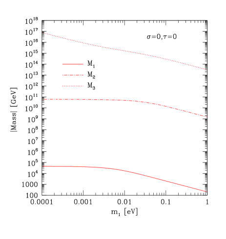
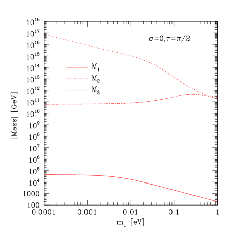
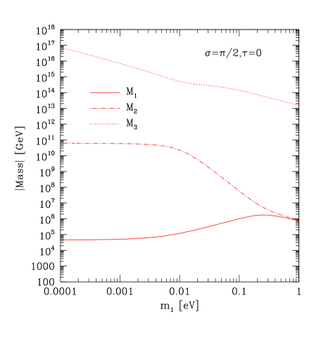
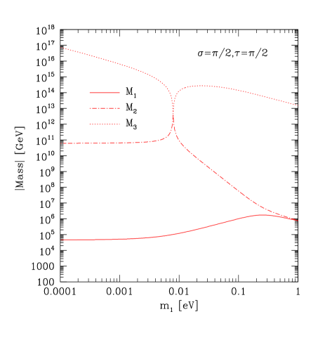
Figure 2: First realization of QLC: the heavy neutrino masses resulting from the diagonalization of Eq. (35) as a function of the smallest neutrino mass for the normal mass ordering. We have chosen four different pairs of values for $\sigma$ and $\tau$, showing the possible degeneracy of the masses. See text for further discussion.

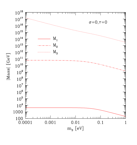
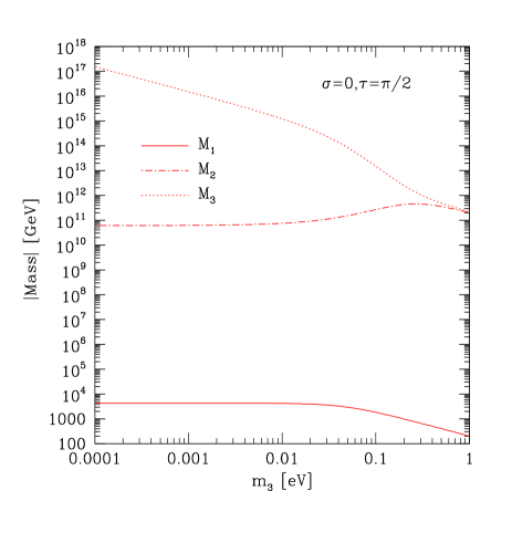
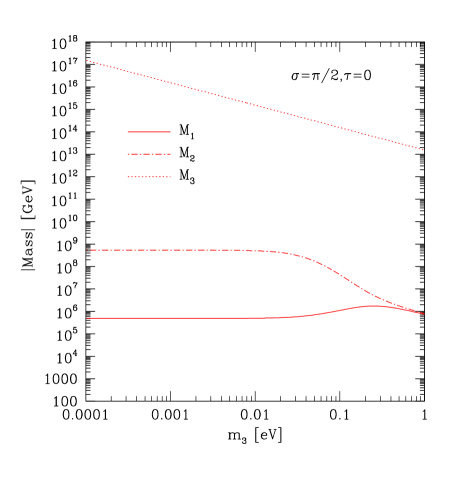
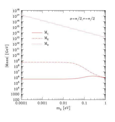
Figure 3: Same as Figure 2 for the inverted mass ordering.

where $R_{\nu}={\rm diag}(e^{-i\phi_{1}/2},e^{-i\phi_{2}/2},e^{-i\phi_{3}/2})$ contains the phases of the eigenvalues in Eq. (36). The above matrix is unitary to order $m_{u}/m_{c}$ or $m_{c}/m_{t}$, which phenomenologically corresponds to an order of $\lambda^{4}$. The heavy neutrino masses are plotted in Fig. 2 as a function of the lightest neutrino mass in case of normal ordering. Figure 3 shows the same for inversely ordered light neutrinos. We have chosen four different pairs of values for $\sigma$ and $\tau$. For the plots we have fixed $\Delta m^{2}_{\odot}$ and $\Delta m^{2}_{\rm A}$ to their best-fit values and have taken the quark masses as $m_{u}=0.45$ MeV, $m_{c}=1.2$ GeV and $m_{t}=175$ GeV. The matrix $M_{R}$ was diagonalized numerically. Eq. (36) is nevertheless an excellent approximation if $\sigma$ and $\tau$ are far away from $\pi/2$. Moreover, it holds that $V_{R}\simeq\mathbbm{1}$ in this case. On the other hand, if $\sigma\simeq\pi/2$ it can occur that $M_{1}$ and $M_{2}$ are almost degenerate if $m_{1}$ takes a value around 0.5 eV. This happens if $\tilde{A}=0$ or, strictly speaking, $\tilde{A}\,m_{u}^{2}\ll\tilde{B}\,m_{u}\,m_{c}$ in which case Eqs. (36, 38) are no longer valid [39, 40], but $M_{1}$ and $M_{2}$ build a pseudo-Dirac pair with mass

$$M_{1}\simeq M_{2}\simeq\tilde{B}\,m_{u}\,m_{c}\simeq\frac{m_{u}\,m_{c}}{2\sqrt{2}\,m_{1}}\sim 10^{6}~{}\rm GeV~{}.$$ (39)

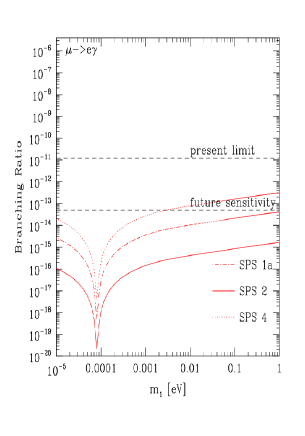
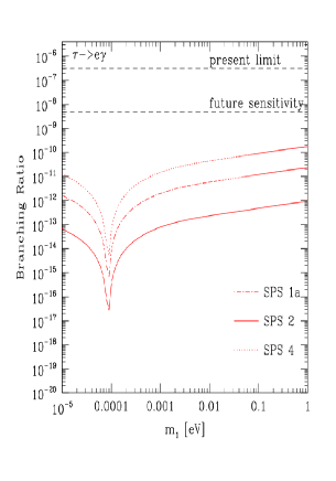
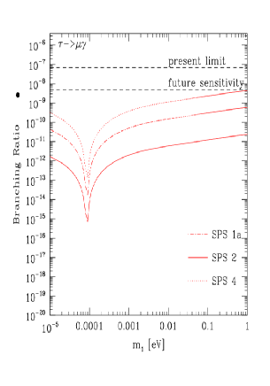
Figure 4: First realization of QLC: the branching ratios for $\mu\rightarrow e\gamma$, $\tau\rightarrow e\gamma$ and $\tau\rightarrow\mu\gamma$ against the smallest neutrino mass (normal ordering) for the SPS points 1a, 2 and 4, see Table 1. Indicated are also the present and future experimental sensitivities.

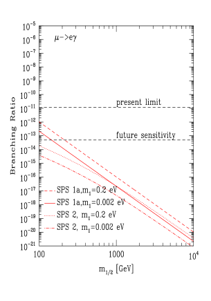
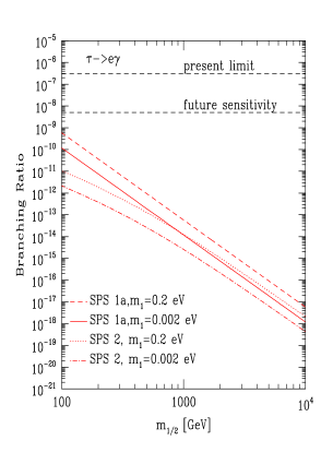
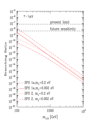
Figure 5: First realization of QLC: the branching ratios for $\mu\rightarrow e\gamma$, $\tau\rightarrow e\gamma$ and $\tau\rightarrow\mu\gamma$ against the SUSY parameter $m_{1/2}$ for the SPS slopes 1a and 2 see Table 1. We have chosen two values for the neutrino masses (normal ordering), namely 0.002 eV and 0.2 eV. Indicated are also the present and future experimental sensitivities.

Note that the indicated value of $m_{1}$ is in conflict with tight cosmological constraints [41]. There are similar situations for $M_{2}$ and $M_{3}$, which occur when $\tau\simeq\pi/2$. Neglecting these tuned cases, we plot the branching ratios in case of $\tau=\sigma=0$ for the normal ordering in Fig. 4 as a function of the smallest neutrino mass, choosing the SPS points 1a, 2 and 4. We do not use points 1b and 3, because the corresponding plots will be indistinguishable from the plots for points 1a and 2, respectively. The results are typical if both $\tau$ and $\sigma$ are not close to $\pi/2$. In order to take renormalization aspects into account, we evaluated the branching ratios for quark masses at high scale [38]. For instance, we took $m_{u}=0.7$ MeV, $m_{c}=210$ MeV and $m_{t}=82.4$ GeV, which corresponds for $\tan\beta=10$ to $m_{u}=2.3$ MeV, $m_{c}=677$ MeV and $m_{t}=181$ GeV at $M_{Z}$ [38]. Due to the presence of the diagonal matrix $L=\delta_{ij}\,\ln M_{X}/M_{i}$ in the equation for the branching ratios the possibility of cancellations arises, leading to a very small branching ratio. From Eq. (32) alone, such a cancellation is impossible. We have also indicated current and future sensitivities on the decays in Fig. 4. Typically, $\mu\rightarrow e\gamma$ can be observable for not too small neutrino masses, unless the SUSY masses approach the TeV scale. BR($\tau\rightarrow e\gamma$) is predicted to be very small, and observation of $\tau\rightarrow\mu\gamma$ requires rather large neutrino masses, small SUSY masses, or large $\tan\beta$. This is illustrated in Fig. 5, where we have plotted the branching ratios as a function of the SUSY parameter $m_{1/2}$ for the SPS slopes 1a and 2 from Table 1. We have chosen two values for the neutrino masses (normal ordering), namely 0.002 eV and 0.2 eV. The relative magnitude of the branching ratios, as estimated in Eq. (34), holds true for most of the parameter space.

3.3 Comments on Leptogenesis

It is worth to discuss leptogenesis in the scenario under study. As indicated in Sec. 2.3, the value of the baryon asymmetry crucially depends on the spectrum of the heavy Majorana neutrinos, which we have displayed in Figs. 2 and 3 for normally and inversely ordered light neutrino masses. It also depends on the matrix $V_{R}$, which in case of $\sigma$ far away from $\pi/2$ is given in Eq. (38). In this case the eigenvalues $M_{1,2,3}$ are strongly hierarchical. In general $M_{1}$ does not exceed $10^{6}$ GeV, as obvious from Eq. (36) and Figs. 2, 3. According to Eq. (18) this is too small a value for successful thermal leptogenesis generated by this heavy neutrino. As pointed out in Section 2.3, it is in principle possible that the second heaviest neutrino generates the decay asymmetry. We will illustrate now that within the QLC scenario under study this is problematic. Taking advantage of the analysis in [30] we can estimate the resulting baryon asymmetry including flavor effects [29, 30]. The decay asymmetry of the neutrino with mass $M_{2}$ in the flavor $\alpha=e,\mu,\tau$ reads [30, 42]

$$\begin{array}[]{c}\varepsilon_{2}^{\alpha}\displaystyle\simeq-\frac{1}{8\pi\,v_{u}^{2}}\,\frac{1}{\left(\tilde{m}_{D}\,\tilde{m}_{D}^{\dagger}\right)_{22}}\left[\frac{3}{2}\,\frac{M_{2}}{M_{3}}\,{\rm Im}\left\{(\tilde{m}_{D})_{2\alpha}\,(\tilde{m}_{D}^{\dagger})_{\alpha 3}\,\left(\tilde{m}_{D}\,\tilde{m}_{D}^{\dagger}\right)_{23}\right\}\right.\\[5.69046pt] \left.\displaystyle+\frac{M_{1}}{M_{2}}\,\left(\ln\frac{M_{2}}{M_{1}}-2\right)\,{\rm Im}\left\{(\tilde{m}_{D})_{2\alpha}\,(\tilde{m}_{D}^{\dagger})_{\alpha 1}\,\left(\tilde{m}_{D}\,\tilde{m}_{D}^{\dagger}\right)_{21}\right\}\right]~{},\end{array}$$ (40)

where $\tilde{m}_{D}$ is given in Eq. (20). In case of a normal hierarchy, we can neglect $m_{1}$ with respect to $m_{2}\simeq\sqrt{\mbox{$\Delta m^{2}_{\odot}$}}$ and $m_{3}\simeq\sqrt{\mbox{$\Delta m^{2}_{\rm A}$}}$ and find from Eq. (36) that

$$\begin{array}[]{c}\displaystyle M_{1}\,e^{i\phi_{1}}\simeq\frac{2\,m_{u}^{2}}{\sqrt{\mbox{$\Delta m^{2}_{\odot}$}}}\,e^{2i\sigma}~{}~{},~{}~{}M_{2}\,e^{i\phi_{2}}\simeq\frac{2\,m_{c}^{2}}{\sqrt{\mbox{$\Delta m^{2}_{\rm A}$}}}\,e^{2i\tau}~{}~{},~{}~{}M_{3}\,e^{i\phi_{3}}\simeq\frac{m_{t}^{2}}{4\,m_{1}}~{},\end{array}$$ (41)

which fixes $\phi_{1}=2\sigma$, $\phi_{2}=2\tau$ and $\phi_{3}=0$ in the phase matrix $R_{\nu}$ appearing in Eq. (38). The matrix $\tilde{V}_{R}$ in Eq. (38) simplifies considerably to

$$\tilde{V}_{R}\simeq\left(\begin{array}[]{ccc}\displaystyle 1&\displaystyle-\frac{m_{u}}{\sqrt{2}\,m_{c}}&\displaystyle\sqrt{2}\,\frac{m_{u}}{m_{t}}\\[8.5359pt] \displaystyle\frac{m_{u}}{\sqrt{2}\,m_{c}}&\displaystyle 1&\displaystyle-\frac{m_{c}}{m_{t}}\\[8.5359pt] \displaystyle-\frac{m_{u}}{\sqrt{2}\,m_{t}}&\displaystyle\frac{m_{c}}{m_{t}}&1\end{array}\right)~{}.$$ (42)

We can evaluate the decay asymmetries by making an expansion in terms of $\lambda$, for which we use that $m_{c}=c_{c}\,m_{t}\,\lambda^{4}$ and $m_{u}=c_{u}\,m_{t}\,\lambda^{8}$ with $c_{u,c}\simeq 1$. One finds that $\varepsilon_{2}^{\tau}$ is larger than $\varepsilon_{2}^{\mu}$ ($\varepsilon_{2}^{e}$) by two (four) orders in $\lambda$. The leading term in $\varepsilon_{2}^{\tau}$ comes from the contribution proportional to $M_{2}/M_{3}\simeq 8\,c_{c}^{2}\,\lambda^{8}\,m_{1}/m_{3}$ in Eq. (40). Thus we obtain

$$\varepsilon_{2}^{\tau}\simeq\frac{3\,c_{c}^{2}}{2\,\pi\,(1+c_{c}^{2})}\,\frac{m_{1}}{\sqrt{\mbox{$\Delta m^{2}_{\rm A}$}}}\,\lambda^{8}\,\sin 2(\omega-\phi+\tau)\simeq 5\cdot 10^{-9}\,\left(\frac{m_{1}}{10^{-4}\,\rm eV}\right)\,\sin 2(\omega-\phi+\tau)~{}.$$ (43)

The second contribution in Eq. (40) proportional to $M_{1}/M_{2}$ is suppressed by $(1-c_{c}^{2})\,\lambda^{24}\,m_{3}/m_{2}$, which is always much smaller than $m_{1}/\sqrt{\mbox{$\Delta m^{2}_{\rm A}$}}\,\lambda^{8}$ due to the lower limit on $m_{1}$ from Eq. (37). We can identify the leptogenesis phase $\omega-\phi+\tau$. This combination of phases is not directly measurable in low energy experiments, as is clear from the results in Section 3.1. Recall however that $\sin^{2}\theta_{23}-\frac{1}{2}\propto\lambda^{2}\,\cos(\omega-\phi)$, $J_{CP}\propto\sin\phi$ and $\sin\beta\simeq-\sin(\phi+\tau)$, which in principle allows to reconstruct the leptogenesis phase with low energy measurements. However, determining the Majorana phases in case of a normal hierarchy seems at present impossible. We still have to estimate the final baryon asymmetry from the decay asymmetry Eq. (43). The wash-out of $\varepsilon_{2}^{\tau}$ by the lightest neutrino is governed by $\tilde{m}_{1}^{\tau}/m^{\ast}$, where $m^{\ast}\simeq 10^{-3}$ eV and $\tilde{m}_{i}^{\tau}\simeq(\tilde{m}_{D})_{i\tau}\,(\tilde{m}_{D}^{\dagger})_{\tau i}/M_{i}$. In our case, $\tilde{m}_{1}^{\tau}/m^{\ast}\simeq\sqrt{\mbox{$\Delta m^{2}_{\odot}$}}/(4\,c_{u}^{2}\,m^{\ast})\simeq 2$, which confirms the result in Ref. [30], where it has been shown that the resulting wash-out is of order 0.2. Without flavor effects, the wash-out would be two orders of magnitude stronger [30], which clearly demonstrates their importance. However, there is very strong wash-out from interactions involving $M_{2}$: the efficiency is $m^{\ast}/\tilde{m}_{2}^{\tau}\simeq 2\,c_{c}^{2}\,m^{\ast}/\sqrt{\mbox{$\Delta m^{2}_{\rm A}$}}\simeq 1/25$ and the estimate for the total baryon asymmetry is [30]

$$\eta_{B}\simeq 6\cdot 10^{-5}\,\epsilon_{2}^{\tau}\simeq 3\cdot 10^{-13}\,\left(\frac{m_{1}}{10^{-4}~{}\rm eV}\right)\,\sin 2(\omega-\phi+\tau)~{},$$ (44)

which is much below the observed value of $6\cdot 10^{-10}$. Of course, these estimates will eventually have to be confirmed by a precise numerical analysis. Nevertheless, it serves to show that successful thermal leptogenesis with the second heaviest Majorana neutrino is quite problematic in the scenario.

We can perform similar estimates if the light neutrinos are governed by an inverted hierarchy. After some algebra in analogy to the normal hierarchical case treated above we find that

$$\begin{array}[]{c}\varepsilon_{2}^{\tau}\simeq\displaystyle\frac{3\,c_{c}^{2}}{16\,\pi\,(1+c_{c}^{2})}\,\frac{m_{3}}{\sqrt{\mbox{$\Delta m^{2}_{\rm A}$}}}\,\lambda^{8}\,\sin 2(\phi+\tau-\omega-\sigma/2)\\ \displaystyle\simeq 7\cdot 10^{-10}\,\left(\frac{m_{3}}{10^{-4}\,\rm eV}\right)\,\sin 2(\phi+\tau-\omega-\sigma/2)~{},\end{array}$$ (45)

which is always larger than $\varepsilon_{2}^{e,\mu}$. This expression is one order of magnitude smaller than the decay asymmetry for the normal hierarchy. It seems therefore that successful leptogenesis within the inverted hierarchy is even more difficult. A more precise statement would require solving the full system of Boltzmann equations. The leptogenesis phase is now $\phi+\tau-\omega-\sigma/2$ and this combination of phases can in principle be reconstructed using $\sin^{2}\theta_{23}-\frac{1}{2}\propto\lambda^{2}\,\cos(\omega-\phi)$, $J_{CP}\propto\sin\phi$, $\sin\beta\simeq-\sin(\phi+\tau)$ and $\sin(\alpha-\beta)\simeq\sin(\phi-\sigma+\tau)$. However, determining both Majorana phases seems at present impossible.

There is another interesting situation in which successful leptogenesis can take place in this scenario, namely resonant leptogenesis. This can occur if $\sigma\simeq\pi/2$, in which case two heavy neutrinos have quasi-degenerate masses, see Eq. (39). In Ref. [40] a similar framework was considered, and the mass splitting required to generate an $\eta_{B}$ of the observed size has been estimated. The result corresponds to $|1-M_{2}/M_{1}|\simeq 10^{-5}\ldots 10^{-6}$, which is a rather fine-tuned situation. However, there are two rather interesting aspects to this case: as discussed in Section 3.1 the phase $\sigma$ is related to the low energy Majorana phase $\alpha$. If $\alpha=\pi/2$ it is known that for quasi-degenerate neutrinos the stability with respect to radiative corrections is significantly improved [24]. Moreover, the resonant condition occurs if the smallest neutrino mass is approximately 0.5 eV, i.e., the light neutrinos are quasi-degenerate. In this case the effective mass for neutrinoless double beta decay reads

$$\mbox{$\langle m\rangle$}\simeq m_{1}\,\left(\sqrt{2}\,\lambda+\frac{1}{2}\,c_{\phi+2\tau}\,\lambda^{2}\right)~{}.$$ (46)

The maximum value of the effective mass for quasi-degenerate neutrinos is roughly $m_{1}$ [36]. The suppression factor $\sqrt{2}\,\lambda$ is nothing but $\cos 2\theta_{12}$. Therefore there are sizable cancellations in the effective mass [44] when the resonance condition for the heavy neutrino masses is fulfilled. With $m_{1}\simeq 0.5$ eV we can predict that $\mbox{$\langle m\rangle$}\simeq 0.16$ eV, a value which can be easily tested in running and up-coming experiments [45].

If $\tau\simeq\pi/2$, it is apparent from Figs. 2 and 3 that situations can occur in which $M_{2}$ and $M_{3}$ are quasi-degenerate. Hence, their decay could create a resonantly enhanced decay asymmetry, but the lighter neutrino with mass $M_{1}$ should not wash out this asymmetry. Determining if this is indeed possible would again require a dedicated study and solution of the Boltzmann equations. Leaving the fine-tuned possibility of resonant leptogenesis aside, we can consider non-thermal leptogenesis. However, as also discussed in Ref. [40], the decay asymmetry $\varepsilon_{1}$ turns out to be too tiny: if we insert the phenomenological values $m_{u}/m_{c}\sim m_{c}/m_{t}\simeq\lambda^{4}$ in the exact equations and if we refrain from considering the possibility of resonant enhancements, $\varepsilon_{1}$ is of order $\lambda^{16}\simeq 10^{-11}$. In principle, the baryon asymmetry could be generated by the decays of the heavier neutrinos, i.e., by $\varepsilon_{2}$ and/or $\varepsilon_{3}$, which are indeed larger than $\varepsilon_{1}$. This possibility would indicate that the inflaton has a sizable branching ratio in the heavier neutrinos. However, this would also require that the lightest Majorana neutrino $N_{1}$ does not wash out the asymmetry generated by $N_{2}$ and $N_{3}$, making a detailed numerical analysis necessary.

4 Second Realization of QLC

In this section we discuss another possible realization of QLC, which has also been outlined already in [5, 6]:

• the conventional see-saw mechanism generates the neutrino mass matrix. Diagonalization of $m_{\nu}$ is achieved via $m_{\nu}=U_{\nu}^{\ast}\,m_{\nu}^{\rm diag}\,U_{\nu}^{\dagger}$ and $U_{\nu}$ is related to $V$ (in the sense that $U_{\nu}^{\dagger}=P_{\nu}\,V\,Q_{\nu}$);

• the matrix diagonalizing the charged leptons corresponds to bimaximal mixing: $U_{\ell}=U_{\rm bimax}^{T}$. This can be achieved when $V_{\rm up}=V^{\dagger}$, therefore $V_{\rm down}=\mathbbm{1}$;

• if indeed $V_{\rm up}=V^{\dagger}$, then $m_{\nu}=-m_{D}^{T}\,M_{R}^{-1}\,m_{D}$ is diagonalized by the CKM matrix. If $M_{R}$ does not introduce additional rotations we can have the $SO(10)$-like relation $m_{\rm up}=m_{D}=V^{\prime}_{\rm up}\,m_{\rm up}^{\rm diag}\,P_{\nu}\,V\,Q_{\nu}$. Here $V^{\prime}_{\rm up}$ denotes in our convention the in principle unknown right-handed rotation of $m_{D}$. The condition of $M_{R}$ not introducing additional rotations means that $V_{R}=(V^{\prime}_{\rm up})^{\ast}$, where $M_{R}=V_{R}^{\ast}\,M_{R}^{\rm diag}\,V_{R}^{\dagger}$.

Note that the equalities $U_{\ell}=U_{\rm bimax}^{T}$ and $V_{\rm down}=\mathbbm{1}$ are consistent with the $SU(5)$-like relation $m_{\ell}=m_{\rm down}^{T}$. The same comments as in the first realization of QLC on whether the indicated scenario is “realistic” or not, would then apply here. If $m_{\ell}=m_{\rm down}^{T}$ was not assumed, the quark and lepton sector would not be related.

In the following we will redo the calculations of the previous sections for all the observables with this second set of assumptions. First of all we note that in the important basis in which the charged leptons and heavy neutrinos are real and diagonal the Dirac mass matrix reads

$$\begin{array}[]{c}m_{D}\rightarrow\tilde{m}_{D}=V_{R}^{T}\,m_{D}\,U_{\ell}=m_{\rm up}^{\rm diag}\,P_{\nu}\,V\,Q_{\nu}\,U_{\rm bimax}^{T}\\[5.69046pt] \Rightarrow\left\{\begin{array}[]{cc}\tilde{m}_{D}^{\dagger}\,\tilde{m}_{D}=U_{\rm bimax}\,Q_{\nu}^{\dagger}\,V^{\dagger}\,{\rm diag}(m_{u}^{2},m_{c}^{2},m_{t}^{2})\,V\,Q_{\nu}\,U_{\rm bimax}^{T}&\mbox{ for LFV}~{},\\[8.5359pt] \tilde{m}_{D}\,\tilde{m}_{D}^{\dagger}={\rm diag}(m_{u}^{2},m_{c}^{2},m_{t}^{2})&\mbox{ for }\eta_{B}~{}.\end{array}\right.\end{array}$$ (47)

The correspondence between the light and heavy Majorana neutrino masses is rather trivial:

$$M_{1}=\frac{m_{u}^{2}}{m_{1}}~{}~{},~{}~{}M_{2}=\frac{m_{c}^{2}}{m_{2}}~{}~{},~{}~{}M_{3}=\frac{m_{t}^{2}}{m_{3}}~{}.$$ (48)

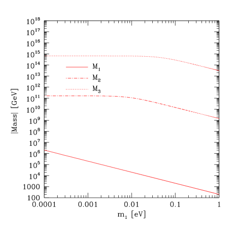
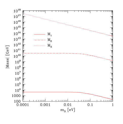
Figure 6: Second realization of QLC: the heavy neutrino masses as a function of the smallest neutrino mass for the normal (left plot) and inverted (right plot) mass ordering.

In Fig. 6 we show the neutrino masses as a function of the smallest neutrino mass $m_{1}$ and $m_{3}$ for the normal and inverted ordering, respectively. Again, we have taken the best-fit points for $\Delta m^{2}_{\odot}$ and $\Delta m^{2}_{\rm A}$ and the quark masses are $m_{u}=0.45$ MeV, $m_{c}=1.2$ GeV and $m_{t}=175$ GeV. Note that in contrast to the first realization of QLC there is no possibility to enhance the neutrino masses, since they do not depend on phases. We can set a lower limit on $m_{1}$ or $m_{3}$ which stems from the requirement that $M_{1}$ or $M_{3}$ does not exceed the Planck mass:

$$m_{1}\geq\frac{m_{u}^{2}}{M_{\rm Pl}}\simeq 8\cdot 10^{-17}~{}{\rm eV}\mbox{ and }m_{3}\geq\frac{m_{t}^{2}}{M_{\rm Pl}}\simeq 2\cdot 10^{-7}~{}{\rm eV}~{}.$$ (49)

This is for $m_{1}$ 10 orders of magnitude smaller than the corresponding limit in the first realization of QLC, see Eq. (37).

Interestingly, there can be no leptogenesis in this scenario. First of all, $M_{1}$ is lighter than $10^{7}$ GeV and this is – in analogy to the first realization of QLC – too small a value for successful leptogenesis. Can the decay of the second heaviest neutrino generate the baryon asymmetry? The answer is no, simply because $\tilde{m}_{D}\,\tilde{m}_{D}^{\dagger}$ is diagonal, as can be seen in Eq. (47). The decay asymmetries, both in the case when one sums over all flavors, Eq. (17), and the asymmetries for a given flavor, Eq. (40), are always proportional to off-diagonal entries of $\tilde{m}_{D}\,\tilde{m}_{D}^{\dagger}$ and therefore always vanish in this realization of QLC.

4.1 Low Energy Neutrino Phenomenology

In our second case the PMNS matrix can be written as

$$U=U_{\ell}^{\dagger}\,U_{\nu}=R_{23}\,R_{12}\,(P_{\nu}\,V\,Q_{\nu})^{\dagger}~{},$$ (50)

where $R_{ij}$ is a rotation with $\pi/4$ around the ($ij$)-axis and $P_{\nu}$ and $Q_{\nu}$ are defined in Eq. (21). We remark that an analysis of this framework including all possible phases has not been performed before (see Refs. [5, 6, 9]). With our parameterization of the PMNS matrix the two phases in $P_{\nu}$ are “Majorana-like” and do not show up in oscillations. All phases originate from the neutrino sector. The neutrino oscillation observables are

$$\begin{array}[]{c}\sin^{2}\theta_{12}=\frac{\displaystyle 1}{\displaystyle 2}-\lambda\,\cos\sigma+{\cal O}(\lambda^{3})~{},\\[5.69046pt] |U_{e3}|=\frac{\displaystyle A}{\displaystyle\sqrt{2}}\,\lambda^{2}+{\cal O}(\lambda^{3})~{},\\[5.69046pt] \sin^{2}\theta_{23}=\frac{\displaystyle 1}{\displaystyle 2}-\sqrt{\frac{1}{2}}\,A\,\lambda^{2}\,\cos(\tau-\sigma)+{\cal O}(\lambda^{3})~{},\\[5.69046pt] J_{CP}^{\rm lep}=\frac{\displaystyle\lambda^{2}}{\displaystyle 4\sqrt{2}}\,\sin(\tau-\sigma)+{\cal O}(\lambda^{3})~{}.\end{array}$$ (51)

The solar neutrino mixing parameter depends on the $CP$ phase $\sigma$. Note that in order to have solar neutrino mixing of the observed magnitude, the phase has to be close to zero or $2\pi$, at $3\sigma$ typically below $\pi/4$ (or above $7\pi/4$). The prediction for $\sin^{2}\theta_{12}$ is

$$\sin^{2}\theta_{12}\mathrel{\hbox to0.0pt{\raise 2.20013pt\hbox{$>$}\hss}{\lower 2.20013pt\hbox{$\sim$}}}0.279~{}(0.278,\,0.277,\,0.276)~{}.$$ (52)

These are lower values than in our first scenario. The numbers have to be compared to the $1\sigma$ ($2\sigma$) limit of $\sin^{2}\theta_{12}\leq 0.33~{}(0.37)$. The parameter $|U_{e3}|$ has a “central value” of $A\,\lambda^{2}/\sqrt{2}\simeq 0.0295$. In the first scenario the prediction was $|U_{e3}|^{2}=0.0258$, which is by chance almost the same number. We find a range of

$$|U_{e3}|=0.0295^{+0.0059,\,0.0070,\,0.0085,\,0.0099}_{-0.0058,\,0.0066,\,0.0076,\,0.0084}~{}.$$ (53)

Recall that the $1\sigma$ ($2\sigma$) bound on $|U_{e3}|$ is 0.11 (0.17). Probing such small values of $|U_{e3}|$ is rather challenging and would require at least superbeams [35]. Due to cancellations $\sin^{2}\theta_{23}=\frac{1}{2}$ can always occur. In this case, $\cos(\tau-\sigma)=0$ and $J_{CP}^{\rm lep}$ takes its maximal possible value. The minimal and maximal values of $\sin^{2}\theta_{23}$ are given by

$$\sin^{2}\theta_{23}\geq 0.466~{}(0.465,\,0.463,\,0.462)~{}\mbox{ and }\sin^{2}\theta_{23}\leq 0.536~{}(0.538,\,0.539,\,0.540)~{},$$ (54)

which is only a slightly larger range compared to the first scenario, and thus hard to probe experimentally. Leptonic $CP$ violation is in leading order proportional to $\lambda^{2}\,\sin(\tau-\sigma)$, which is four powers of $\lambda$ larger than the $J_{CP}$ of the quark sector. If the neutrino sector conserved $CP$, then $J_{CP}^{\rm lep}$ vanishes. Note that the phase combination ($\tau-\sigma$) governs the magnitude of the atmospheric neutrino mixing. In the first scenario, $J_{CP}^{\rm lep}$ and the solar neutrino mixing were correlated in this way. In analogy to Eq. (25) we can write the sum-rule

$$\begin{array}[]{c}\sin^{2}\theta_{23}\simeq\frac{1}{2}-|U_{e3}|\,\cos(\tau-\sigma)\simeq\frac{1}{2}\pm\sqrt{|U_{e3}|-16\,J_{CP}^{2}}~{}.\end{array}$$ (55)

In Fig. 7 we show the correlations between the oscillation parameters which result from the relation in Eq. (50). We plot $J_{CP}^{\rm lep}$ and $\sin^{2}\theta_{12}$ against $\sin^{2}\theta_{23}$, as well as $\sigma$ and $|U_{e3}|$ against $\sin^{2}\theta_{12}$. We also indicate the current 1, 2 and $3\sigma$ ranges of the oscillation parameters, showing that the predictions of this scenario are perfectly compatible with all current data.

Turning aside again from the oscillation observables, the invariants for the Majorana phases are

$$S_{1}=-\frac{\displaystyle\lambda^{2}}{\displaystyle 2}\,A\,\sin(\sigma+\omega)+{\cal O}(\lambda^{3})\mbox{ and }S_{2}=-\frac{\displaystyle\lambda^{2}}{\displaystyle 2}\,A\,\sin(\omega-\phi)+{\cal O}(\lambda^{3})~{}.$$ (56)

In analogy to the discussion following Eq. (27), we can translate these formulae into expressions for the low energy Majorana phases $\alpha$ and $\beta$. This leads to $\sin\beta\simeq\sin(\sigma+\omega)$ and $\sin(\alpha-\beta)\simeq\sin(\phi-\omega)$ and indicates that $\alpha$ in the parameterization of Eq. (6) is related to ($\phi+\sigma$). Indeed, a calculation of the effective mass in case of an inverted hierarchy, where the Majorana phase $\alpha$ plays a crucial role [36], results in

$$\mbox{$\langle m\rangle$}\simeq\sqrt{\mbox{$\Delta m^{2}_{\rm A}$}}\,\left|c_{\phi+\sigma}+2\frac{s_{\phi}}{c_{\phi+\sigma}}\lambda^{2}\right|~{}.$$ (57)

Similar statements can be made for quasi-degenerate neutrinos.

4.2 Lepton Flavor Violation

With the help of Eqs. (13, 47) we can evaluate the branching ratios for LFV processes, ignoring for the moment the logarithmic dependence on the heavy neutrino masses. The decay $\mu\rightarrow e\gamma$ is found to be governed by

$$\left|(\tilde{m}_{D}^{\dagger}\,\tilde{m}_{D})_{21}\right|^{2}\simeq\frac{1}{4}\,A^{2}\,m_{t}^{4}\,\lambda^{4}+{\cal O}(\lambda^{5})~{}.$$ (58)

Comparing with Eq. (32) we see that in the second realization the branching ratio is larger than in the first realization by 6 inverse powers of $\lambda$, or $\lambda^{-6}\simeq 8820$, almost 4 orders of magnitude. For the double ratios of the branching ratios we obtain

$$R(21/31)\simeq 1-2\sqrt{2}\,A\,\cos(\sigma-\tau)\,\lambda^{2}+{\cal O}(\lambda^{3})~{}~{},~{}~{}R(21/32)\simeq A^{2}\,\lambda^{4}+{\cal O}(\lambda^{5})~{}.$$ (59)

There is a small dependence on the phase combination ($\sigma-\tau$), which also governs leptonic $CP$ violation in oscillation experiments and the magnitude of the atmospheric neutrino mixing angle. The branching ratios behave according to

$$\text{BR}(\mu\rightarrow e\gamma):\text{BR}(\tau\rightarrow e\gamma):\text{BR}(\tau\rightarrow\mu\gamma)\simeq A^{2}\,\lambda^{4}:A^{2}\,\lambda^{4}:1~{}.$$ (60)

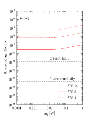
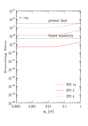
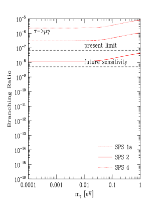
Figure 8: Second realization of QLC: the branching ratios for $\mu\rightarrow e\gamma$, $\tau\rightarrow e\gamma$ and $\tau\rightarrow\mu\gamma$ against the smallest neutrino mass (normal ordering) for the SPS points 1a, 2 and 4, see Table 1. Indicated are also the present and future sensitivities.

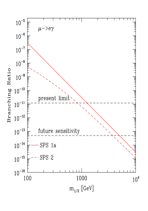
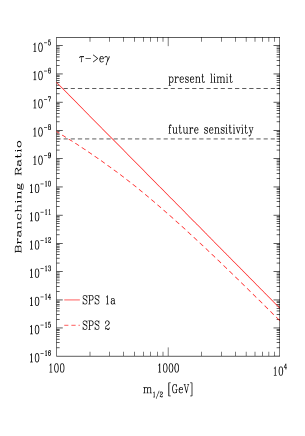
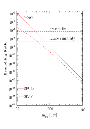
Figure 9: Second realization of QLC: the branching ratios for $\mu\rightarrow e\gamma$, $\tau\rightarrow e\gamma$ and $\tau\rightarrow\mu\gamma$ against the SUSY parameter $m_{1/2}$ for the SPS slopes 1a and 2, see Table 1. We have chosen for the neutrino mass (normal ordering) 0.02 eV. Indicated are also the present and future sensitivities.

In Fig. 8 we show the branching ratios for $\mu\rightarrow e\gamma$, $\tau\rightarrow e\gamma$ and $\tau\rightarrow\mu\gamma$ as a function of the smallest neutrino mass for a normal mass ordering, choosing the SPS points 1a, 2 and 4. The small dependence on the heavy neutrino masses is taken into account and plots for the inverted ordering look very similar. Note that from Fig. 8 it follows that the dependence on the neutrino masses is very small. The relative magnitude of the branching ratios, as estimated in Eq. (59), holds true to a very high accuracy. However, we immediately see that the prediction for $\mu\rightarrow e\gamma$ is at least one order of magnitude above the current limit. To obey the experimental limit on BR($\mu\rightarrow e\gamma$), the SUSY masses should be in the several TeV range. This is illustrated in Fig. 9, where we have plotted the branching ratios as a function of the SUSY parameter $m_{1/2}$ for the SPS slopes 1a and 2 from Table 1. We took the normal ordering of neutrino masses with a smallest mass $m_{1}=0.02$ eV. Once we have adjusted the SUSY parameters to have BR($\mu\rightarrow e\gamma$) below its current limit, the other decays $\tau\rightarrow e\gamma$ and $\tau\rightarrow\mu\gamma$ are too rare to be observed with presently planned experiments.

5 Conclusions and Summary

We have considered the phenomenology of two predictive see-saw scenarios leading approximately to Quark-Lepton Complementarity. Both have in common that bimaximal mixing is corrected by the CKM matrix. We have studied the complete low energy phenomenology, including the neutrino oscillation parameters, where we have taken into account all possible phases, and neutrinoless double beta decay. Moreover, lepton flavor violating charged lepton decays have been studied and all results have been compared to presently available and expected future data. Finally, we have commented on the possibility of leptogenesis .

In terms of the elements of the PMNS matrix $U$ and the CKM matrix $V$, the QLC condition can be written as $|U_{e2}|+|V_{ud}|=1/\sqrt{2}$. This defines the solar neutrino mixing parameter $\sin^{2}\theta_{12}$ to be $\sin^{2}(\frac{\pi}{4}-\lambda)$. Taking the best-fit, as well as the 1, 2 and 3$\sigma$ values of $\lambda$ from Eq. (9) we obtain

$$\sin^{2}\theta_{12}=0.2805\pm(0.0009,\,0.0018,\,0.0027)~{}.$$ (61)

A second QLC relation has also been suggested, namely $\theta_{23}+A\,\lambda^{2}=\pi/4$, which is the analogue of Eq. (2) for the (23)-sector. This can also be written as $|U_{\mu 3}|+|V_{cb}|=1/\sqrt{2}$ and its precise prediction is

$$\sin^{2}\theta_{23}=0.4583^{+0.0011,\,0.0022,\,0.0032}_{-0.0011,\,0.0022,\,0.0034}~{}.$$ (62)

We remark that in our scenario with all possible $CP$ phases the above two relations correspond to at least one phase being zero.

The first scenario has bimaximal mixing from the neutrino sector and the matrix diagonalizing the charged leptons is the CKM matrix. The main results are:

• solar neutrino mixing is predicted close to its 1$\sigma$ bound and $|U_{e3}|$ even close to its 2$\sigma$ bound, see Fig. 1. The phase governing the magnitude of $\theta_{12}$ is the $CP$ phase of neutrino oscillations and is implied to be small;

• $|U_{e3}|$ is roughly 0.16, i.e., it should be observed soon;

• the lowest value of $\sin^{2}\theta_{12}$ (corresponding to $CP$ conservation) is roughly 0.33, which differs by about 15% from Eq. (61). For $\sin^{2}\theta_{23}$ the lowest value is 0.44, in moderate agreement with Eq. (62);

• the decay $\mu\rightarrow e\gamma$ can be observable for not too small neutrino masses, unless the SUSY masses approach the TeV scale. BR($\tau\rightarrow e\gamma$) is predicted to be very small, and observation of $\tau\rightarrow\mu\gamma$ requires rather large neutrino masses, small SUSY masses, or large $\tan\beta$. The relative magnitude of the branching ratios is $\text{BR}(\mu\rightarrow e\gamma):\text{BR}(\tau\rightarrow e\gamma):\text{BR}(\tau\rightarrow\mu\gamma)\simeq\lambda^{6}:\lambda^{2}:1$;

• successful resonant leptogenesis depends on the low energy Majorana phases but is fine-tuned. One possibility occurs if $\sigma\simeq\pi/2$, leading to two quasi-degenerate heavy neutrinos masses. It also leads to quasi-degenerate light neutrinos with mass around 0.5 eV and to sizable cancellations in neutrinoless double beta decay , corresponding to $\mbox{$\langle m\rangle$}\simeq 0.16$ eV. Leptogenesis via the decay of the second heaviest neutrino typically fails, even with the inclusion of flavor effects.

The second scenario has bimaximal mixing from the charged lepton sector and the matrix diagonalizing the neutrinos is the CKM matrix. The main results are:

• the neutrino oscillation parameters are perfectly compatible with all data, see Fig. 7. The phase governing the magnitude of $\theta_{23}$ is the $CP$ phase of neutrino oscillations;

• $|U_{e3}|$ is roughly 0.03, which is a rather small value setting a challenge for future experiments;

• the lowest value of $\sin^{2}\theta_{12}$ (corresponding to $CP$ conservation) is roughly 0.28, in perfect agreement with Eq. (61). For $\sin^{2}\theta_{23}$ the lowest value is 0.46 (but $\theta_{23}$ can be maximal), in perfect agreement with Eq. (62). If $\sin^{2}\theta_{23}=\frac{1}{2}$ then maximal $CP$ violation is implied;

• The branching ratio of $\mu\rightarrow e\gamma$ is larger than in the first scenario by six inverse powers of $\lambda$ and therefore typically too large unless the SUSY masses are of several TeV scale. If they are so heavy that $\mu\rightarrow e\gamma$ is below its current limit, $\tau\rightarrow e\gamma$ and $\tau\rightarrow\mu\gamma$ are too small to be observed. The relative magnitude of the branching ratios is $\text{BR}(\mu\rightarrow e\gamma):\text{BR}(\tau\rightarrow e\gamma):\text{BR}(\tau\rightarrow\mu\gamma)\simeq A^{2}\,\lambda^{4}:A^{2}\,\lambda^{4}:1$;

• there can be no leptogenesis.

We conclude that both scenarios predict interesting and easily testable phenomenology. However, the first scenario is in slight disagreement with oscillation data and allows leptogenesis only for fine-tuned parameter values. In the second scenario the predictions for LFV decays are in contradiction to experimental results unless the SUSY parameters are very large. Moreover no leptogenesis is possible in this case.

Acknowledgments

We are grateful to Stéphane Lavignac for helpful discussions and thank J. Klinsmann for invaluable encouragement. This work was supported by the “Deutsche Forschungsgemeinschaft” in the “Sonderforschungsbereich 375 für Astroteilchenphysik” and under project number RO–2516/3–1 (W.R.).

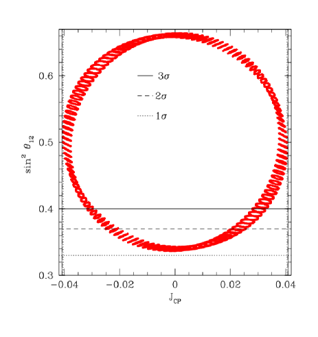
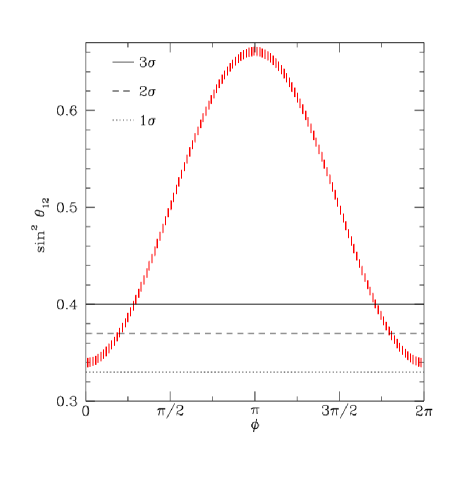
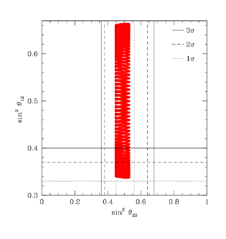
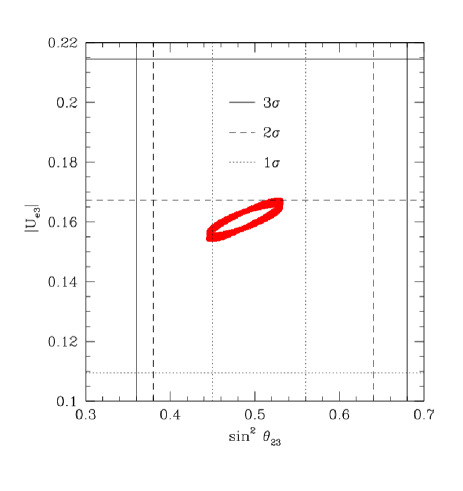
Figure 1: First realization of QLC: neutrino observables resulting from Eq. (22) for the 3$\sigma$ ranges of the CKM parameters. We also indicated the present 1, 2 and 3$\sigma$ ranges of the oscillation parameters.

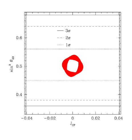
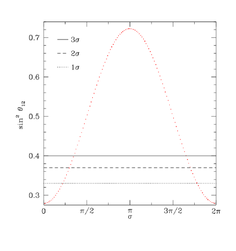
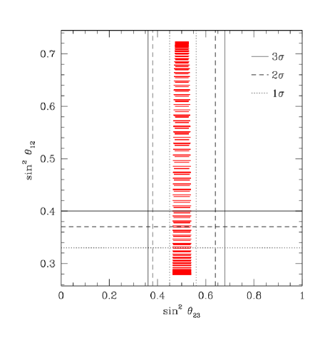
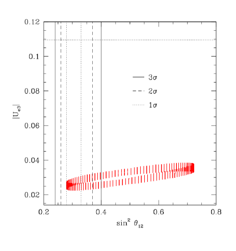
Figure 7: Second realization of QLC: neutrino observables resulting from Eq. (51) for the 3$\sigma$ ranges of the CKM parameters. We also indicated the current 1, 2 and 3$\sigma$ ranges of the oscillation parameters.

References

- [1] R. N. Mohapatra et al., hep-ph/0510213; R. N. Mohapatra and A. Y. Smirnov, hep-ph/0603118; A. Strumia and F. Vissani, hep-ph/0606054.
- [2] W. Rodejohann, Phys. Rev. D 69, 033005 (2004).
- [3] F. Vissani, hep-ph/9708483; V. D. Barger, S. Pakvasa, T. J. Weiler and K. Whisnant, Phys. Lett. B 437, 107 (1998); A. J. Baltz, A. S. Goldhaber and M. Goldhaber, Phys. Rev. Lett. 81, 5730 (1998); H. Georgi and S. L. Glashow, Phys. Rev. D 61, 097301 (2000); R. N. Mohapatra and S. Nussinov, Phys. Rev. D 60, 013002 (1999); I. Stancu and D. V. Ahluwalia, Phys. Lett. B 460, 431 (1999).
- [4] T. Schwetz, Acta Phys. Polon. B 36, 3203 (2005), hep-ph/0510331; M. Maltoni et al., New J. Phys. 6, 122 (2004), hep-ph/0405172v5.
- [5] M. Raidal, Phys. Rev. Lett. 93, 161801 (2004).
- [6] H. Minakata and A. Y. Smirnov, Phys. Rev. D 70, 073009 (2004).
- [7] P. H. Frampton and R. N. Mohapatra, JHEP 0501, 025 (2005); S. K. Kang, C. S. Kim and J. Lee, Phys. Lett. B 619, 129 (2005); N. Li and B. Q. Ma, Phys. Rev. D 71, 097301 (2005); K. Cheung et al., Phys. Rev. D 72, 036003 (2005); Z. Z. Xing, Phys. Lett. B 618, 141 (2005); A. Datta, L. Everett and P. Ramond, Phys. Lett. B 620, 42 (2005); S. Antusch, S. F. King and R. N. Mohapatra, Phys. Lett. B 618, 150 (2005); N. Li and B. Q. Ma, Eur. Phys. J. C 42, 17 (2005); T. Ohlsson, Phys. Lett. B 622, 159 (2005); D. Falcone, Mod. Phys. Lett. A 21, 1815 (2006); L. L. Everett, Phys. Rev. D 73, 013011 (2006); A. Dighe, S. Goswami and P. Roy, Phys. Rev. D 73, 071301 (2006); B. C. Chauhan et al., hep-ph/0605032; F. Gonzalez-Canales and A. Mondragon, hep-ph/0606175.
- [8] J. Ferrandis and S. Pakvasa, Phys. Lett. B 603, 184 (2004); Phys. Rev. D 71, 033004 (2005).
- [9] C. A. de S. Pires, J. Phys. G 30, B29 (2004); N. Li and B. Q. Ma, Eur. Phys. J. C 42, 17 (2005).
- [10] M. Jezabek and Y. Sumino, Phys. Lett. B 457, 139 (1999); Z. Z. Xing, Phys. Rev. D 64, 093013 (2001); C. Giunti and M. Tanimoto, Phys. Rev. D 66, 053013 (2002); Phys. Rev. D 66, 113006 (2002); S. T. Petcov and W. Rodejohann, Phys. Rev. D 71, 073002 (2005); J. Ferrandis and S. Pakvasa, Phys. Lett. B 603, 184 (2004); S. Antusch and S. F. King, Phys. Lett. B 631, 42 (2005).
- [11] P. H. Frampton, S. T. Petcov and W. Rodejohann, Nucl. Phys. B 687, 31 (2004).
- [12] P. Minkowski, Phys. Lett. B 67, 421 (1977); M. Gell-Mann, P. Ramond, and R. Slansky in Supergravity, p. 315, edited by F. Nieuwenhuizen and D. Friedman, North Holland, Amsterdam, 1979; T. Yanagida, Proc. of the Workshop on Unified Theories and the Baryon Number of the Universe, edited by O. Sawada and A. Sugamoto, KEK, Japan 1979; R. N. Mohapatra and G. Senjanovic, Phys. Rev. Lett. 44, 912 (1980).
- [13] S. M. Bilenky, J. Hosek and S. T. Petcov, Phys. Lett. B 94, 495 (1980); J. Schechter and J. W. F. Valle, Phys. Rev. D 22, 2227 (1980); Phys. Rev. D 23, 1666 (1981); M. Doi et al., Phys. Lett. B 102, 323 (1981).
- [14] L. Wolfenstein, Phys. Rev. Lett. 51, 1945 (1983).
- [15] J. Charles et al. [CKMfitter Group], Eur. Phys. J. C 41, 1 (2005); A. Hocker and Z. Ligeti, hep-ph/0605217.
- [16] C. Jarlskog, Phys. Rev. Lett. 55, 1039 (1985).
- [17] J. F. Nieves and P. B. Pal, Phys. Rev. D 36, 315 (1987); Phys. Rev. D 64, 076005 (2001); J. A. Aguilar-Saavedra and G. C. Branco, Phys. Rev. D 62, 096009 (2000).
- [18] S. T. Petcov, Sov. J. Nucl. Phys. 25, 340 (1977) [Yad. Fiz. 25, 641 (1977 ERRAT,25,698.1977 ERRAT,25,1336.1977)]; S. M. Bilenky, S. T. Petcov and B. Pontecorvo, Phys. Lett. B 67, 309 (1977); T. P. Cheng and L. F. Li, Phys. Rev. Lett. 45, 1908 (1980).
- [19] F. Borzumati and A. Masiero, Phys. Rev. Lett. 57, 961 (1986); J. Hisano, T. Moroi, K. Tobe and M. Yamaguchi, Phys. Rev. D 53, 2442 (1996); J. A. Casas and A. Ibarra, Nucl. Phys. B 618, 171 (2001).
- [20] M. L. Brooks et al. [MEGA Collaboration], Phys. Rev. Lett. 83, 1521 (1999).
- [21] L. M. Barkov et al., the MEG Proposal (1999), http://meg.psi.ch.
- [22] S. T. Petcov et al., Nucl. Phys. B 676, 453 (2004).
- [23] B. C. Allanach et al., Eur. Phys. J. C 25, 113 (2002) [eConf C010630, P125 (2001)].
- [24] See for instance S. Antusch et al., JHEP 0503, 024 (2005).
- [25] D. N. Spergel et al., astro-ph/0603449.
- [26] M. Fukugita and T. Yanagida, Phys. Lett. B 174, 45 (1986).
- [27] W. Buchmüller, P. Di Bari and M. Plümacher, New J. Phys. 6, 105 (2004), hep-ph/0406014.
- [28] G. F. Giudice et al., Nucl. Phys. B 685, 89 (2004).
- [29] R. Barbieri et al., Nucl. Phys. B 575, 61 (2000); A. Pilaftsis and T. E. J. Underwood, Phys. Rev. D 72, 113001 (2005); T. Endoh, T. Morozumi and Z. H. Xiong, Prog. Theor. Phys. 111, 123 (2004); T. Fujihara et al., Phys. Rev. D 72, 016006 (2005); A. Abada et al., JCAP 0604, 004 (2006); E. Nardi, Y. Nir, E. Roulet and J. Racker, JHEP 0601, 164 (2006); A. Abada et al., hep-ph/0605281; S. Blanchet and P. Di Bari, hep-ph/0607330; S. Antusch, S. F. King and A. Riotto, hep-ph/0609038; S. Pascoli, S. T. Petcov and A. Riotto, hep-ph/0609125; G. C. Branco, R. G. Felipe and F. R. Joaquim, hep-ph/0609297.
- [30] O. Vives, Phys. Rev. D 73, 073006 (2006).
- [31] M. Flanz, E. A. Paschos and U. Sarkar, Phys. Lett. B 345, 248 (1995) [Erratum-ibid. B 382, 447 (1996)]; M. Flanz, E. A. Paschos, U. Sarkar and J. Weiss, Phys. Lett. B 389, 693 (1996); A. Pilaftsis, Phys. Rev. D 56, 5431 (1997); W. Buchmüller and M. Plümacher, Phys. Lett. B 431, 354 (1998); E. Roulet, L. Covi and F. Vissani, Phys. Lett. B 424, 101 (1998); A. Pilaftsis and T. E. J. Underwood, Nucl. Phys. B 692, 303 (2004); A. Anisimov, A. Broncano and M. Plümacher, Nucl. Phys. B 737, 176 (2006).
- [32] G. Lazarides and Q. Shafi, Phys. Lett. B 258, 305 (1991); K. Kumekawa, T. Moroi and T. Yanagida, Prog. Theor. Phys. 92, 437 (1994); G. F. Giudice, M. Peloso, A. Riotto and I. Tkachev, JHEP 9908, 014 (1999); T. Asaka, K. Hamaguchi, M. Kawasaki and T. Yanagida, Phys. Lett. B 464, 12 (1999); Phys. Rev. D 61, 083512 (2000); T. Asaka, H. B. Nielsen and Y. Takanishi, Nucl. Phys. B 647, 252 (2002).
- [33] K. Cheung et al., in Ref. [7].
- [34] H. Georgi and C. Jarlskog, Phys. Lett. B 86, 297 (1979).
- [35] For an overview on future experiments and their sensitivity, see e.g., A. Blondel et al., hep-ph/0606111; S. Choubey, hep-ph/0509217.
- [36] Recent analyzes of neutrinoless double beta decay are: S. Pascoli, S. T. Petcov and T. Schwetz, Nucl. Phys. B 734, 24 (2006); S. Choubey and W. Rodejohann, Phys. Rev. D 72, 033016 (2005); A. de Gouvea and J. Jenkins, hep-ph/0507021; M. Lindner, A. Merle and W. Rodejohann, Phys. Rev. D 73, 053005 (2006).
- [37] D. Falcone and F. Tramontano, Phys. Rev. D 63, 073007 (2001); G. C. Branco, R. Gonzalez Felipe, F. R. Joaquim and M. N. Rebelo, Nucl. Phys. B 640, 202 (2002); D. Falcone, Phys. Rev. D 68, 033002 (2003).
- [38] C. R. Das and M. K. Parida, Eur. Phys. J. C 20, 121 (2001).
- [39] E. Nezri and J. Orloff, JHEP 0304, 020 (2003).
- [40] E. K. Akhmedov, M. Frigerio and A. Y. Smirnov, JHEP 0309, 021 (2003).
- [41] For a recent review, see S. Hannestad, hep-ph/0602058.
- [42] P. Di Bari, Nucl. Phys. B 727, 318 (2005).
- [43] P. Hosteins, S. Lavignac and C. A. Savoy, hep-ph/0606078.
- [44] W. Rodejohann, Nucl. Phys. B 597, 110 (2001).
- [45] C. Aalseth et al., hep-ph/0412300.