Distribution of multiple scatterings in
proton-nucleus collisions at high energy

Abstract

We consider proton-nucleus collisions at high energy in the Color Glass Condensate framework, and extract from the gluon production cross-section the probabilities of having a definite number of multiple scatterings in the nucleus. Various properties of the distribution of the number of multiple scatterings are studied, and we conclude that events in which the momentum of a hard jet is compensated by many much softer particles on the opposite side are very unlikely except for extreme values of the saturation momentum. In the same framework, we also investigate the possibility to estimate the impact parameter of a proton-nucleus collision, from the measure of the multiplicity of its final state.

1. Theory Group, Physics Department
   CERN
   CH-1211 Geneva 23, Switzerland

2. Service de Physique Théorique (URA 2306 du CNRS)
   CEA/DSM/Saclay, Bât. 774
   91191, Gif-sur-Yvette Cedex, France

Preprint CERN-PH-TH/2006-126, SPhT-T06/075

1 Introduction

Hadronic collisions at high energy involve the interaction of partons that carry a very small fraction $x$ of the longitudinal momentum of the incoming projectile. Since the occupation number for such states in the nucleon wave function can become quite large, one expects that the physics of parton saturation [1, 2, 3] plays an important role in such studies. This saturation generally has the effect of reducing the number of produced particles compared to what one would have predicted on the basis of a pQCD calculation with parton densities that depend on $x$ according to the linear BFKL (Balitsky–Fadin–Kuraev–Lipatov) [4, 5] evolution equation.

The counterpart of such a large occupation number is that one can treat the small-$x$ partons by classical color fields instead of particles. To that effect, the McLerran-Venugopalan model [6, 7, 8] is a hybrid description, in which the small-$x$ partons are described by classical fields, and where the large-$x$ partons – fast and therefore frozen by time dilation – are described as static color sources at the origin of the classical fields, in agreement with the fact that small-$x$ partons are radiated by bremsstrahlung from the large-$x$ ones. Originally, the MV model dealt with large nuclei, with a large number of high-$x$ partons (the number of valence quarks is $3A$ if $A$ is the atomic number of the nucleus). In the MV model, the large-$x$ color sources are described by a statistical distribution, which they argued could be taken to be a Gaussian for a large nucleus at moderately small $x$ (see also [9] for a recent discussion of this point).

Since these early days, this model has become an effective theory, the so-called “Color Glass Condensate” (CGC) [10, 11, 12]. Since the separation between large $x$ and small $x$ is arbitrary, no physical quantity should depend on it. This arbitrariness leads to a renormalization group equation, the so-called JIMWLK (Jalilian-Marian–Iancu–McLerran–Weigert–Leonidov–Kovner) equation [13, 14, 15, 16, 17, 18, 19, 10, 11, 12], that describes how the statistical distribution of color sources changes as one moves the separation between large and small $x$. This functional evolution equation can also be expressed as an infinite hierarchy of evolution equations for correlators [20], and has a quite useful – and much simpler – large $N_{c}$ mean-field approximation [21], known as the Balitsky-Kovchegov equation.

In the collision of two nuclei at high energy, gluon production is dominated by the classical field approximation, and calculating it requires to solve the classical Yang-Mills equations for two color sources – one for each projectile – moving at the speed of light in opposite directions. This problem has been studied numerically in [22, 23, 24, 25, 26] for the boost-invariant case, with extensions to include the rapidity dependence [27, 28]. But in fact, for collisions involving one small projectile – like proton-nucleus collisions – one can assume that the color sources that describe this small projectile are weak and compute the relevant amplitude only at lowest order in this source. When this is allowed, it is possible to obtain analytical expressions for amplitudes and cross-sections. This was done in a number of approaches for single quark or gluon production [29, 30, 31, 32, 33, 34, 35, 36, 37, 38], as well as for quark-antiquark production [39, 40, 41, 42, 43, 44, 45, 46, 47, 48] (see [49] for a review). In this paper, we are going to limit our discussion to the case of single gluon production.

One of the main features of the gluon production cross-section in proton-nucleus obtained in the CGC framework is that it includes all the multiple scatterings on the sources contained in the nucleus. In this paper, we discuss the distribution in the number of these scatterings. In particular, we study how the momentum of a high-$p_{\perp}$ final gluon is balanced by the recoiling momenta of the struck nuclear color sources. This question has practical applications in discussing whether one could observe a loss of back-to-back correlations at high $p_{\perp}$ – for instance events with a single high-momentum jet in the final state – in collisions between a proton and a saturated nucleus. Another application of our study occurs when one tries to relate the multiplicity and the impact parameter of the collision. And of course, one may also try to characterize the nuclear partonic content at low $x$ from the distribution of “debris” that are produced in the collision with the proton.

Note that the manifestations of the Color Glass Condensate on the back-to-back correlations have already been investigated in various approaches [47, 50], by looking at the angular correlations between pairs of hard particles. This azimuthal correlation has been measured for deuteron-gold collisions by the STAR collaboration at RHIC [51], which observed that the pattern of azimuthal correlations in d–Au collisions is very similar to that found in pp collisions. In particular, it has a marked peak in the correlation function at $180$ degrees – indicating that jets come in pairs. In the present paper, we address a different question, which involves most of the same physics: we do not consider the angle of emission of the particles, but instead we keep track of the number of recoils above a certain threshold $k_{\perp}^{\rm min}$ given a “trigger” particle with momentum $k_{\perp}$, and we calculate the probability for having a given number of such recoils.

Our paper is organized as follows. In section 2, we recall the CGC formula for gluon production in proton-nucleus collisions, and we also discuss the Glauber interpretation of this formula. In section 3, we show how to calculate the probability $P_{n}$ of having $n$ scatterings in which the recoil momentum is larger than a certain threshold $k_{\perp}^{\rm min}$, when the produced gluon has acquired the momentum $k_{\perp}$ in the nucleus. This is done by constructing a generating function for these probabilities. In section 4, we present numerical results for this distribution in the MV model, as well as simple analytical calculations that explain the most salient features; and in section 5 we compare them with what happens in a model that has shadowing and geometrical scaling. Finally, in section 6, we discuss the possibility of estimating the impact parameter of the collision from the multiplicity in the final state.

2 Gluon production in proton-nucleus collisions

Here, we use without rederiving it the formula for the gluon yield obtained in [36] (Eq. (107)). According to this formula, the number of gluons produced per unit of transverse momentum and per unit of rapidity reads:

$$\frac{d\overline{N}_{g}}{d^{2}{\boldsymbol{q}}_{\perp}dy}=\frac{1}{16\pi^{3}q_{\perp}^{2}}\int\frac{d^{2}{\boldsymbol{k}}_{\perp}}{(2\pi)^{2}}k_{\perp}^{2}C({\boldsymbol{k}}_{\perp})\,\varphi_{p}({\boldsymbol{q}}_{\perp}-{\boldsymbol{k}}_{\perp})\;,$$ (1)

where $\varphi_{p}$ is the proton non-integrated gluon distribution, that we won’t need to specify further in the following. The function $C(k_{\perp})$, introduced in [52], is the Fourier transform of a correlator of Wilson lines:

$$C(k_{\perp})\equiv\int d^{2}{\boldsymbol{x}}_{\perp}e^{i{\boldsymbol{k}}_{\perp}\cdot{\boldsymbol{x}}_{\perp}}\;\frac{1}{N_{c}^{2}-1}\,{\rm Tr}\,\left<U^{\dagger}(0)U({\boldsymbol{x}}_{\perp})\right>\;.$$ (2)

$U({\boldsymbol{x}}_{\perp})$ is a Wilson line in the adjoint representation of $SU(N_{c})$, evaluated in the color field produced by the sources that describe the nucleus, and the brackets $\big{<}\cdots\big{>}$ denote an averaging over these color sources. Equation (1) is accurate to the lowest order in the density of color sources contained in the proton, and to all orders in the color density of the nucleus. Thus, a way to picture its content is to say that a gluon of the wave-function of the proton travels through the color field of the nucleus before being produced.

At first sight, it looks like the process taken into account by Eq. (1) is a $2\to 1$ process, in which one gluon from the proton (with transverse momentum ${\boldsymbol{q}}_{\perp}-{\boldsymbol{k}}_{\perp}$) merges with a gluon from the nucleus (with transverse momentum ${\boldsymbol{k}}_{\perp}$) in order to produce the final gluon of transverse momentum ${\boldsymbol{q}}_{\perp}$. One might therefore be tempted to conclude that the Color Glass Condensate predicts the production of monojets in proton-nucleus collisions. However, this conclusion is too simplistic. The first reason is of course that transverse momentum is conserved in the CGC framework. This means that if the final gluon has acquired a large momentum ${\boldsymbol{k}}_{\perp}$ while going through the nucleus, this momentum must come from the color sources present in the nucleus. In other words, if one sums the recoil transverse momenta of the sources struck by the propagating gluon, they must add up to $-{\boldsymbol{k}}_{\perp}$.

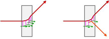
Figure 1: Two possible scenarios for the recoiling scattering centers in the production of a high-$p_{\perp}$ particle. Left: the large $p_{\perp}$ of the produced particle is compensated by many semi-hard recoils. Right: one recoil absorbs almost all the $p_{\perp}$.

Therefore, the real issue in order to conclude about the possible existence of monojets is whether the recoil momentum is shared among many sources (each of them acquiring only a small momentum), or on the contrary absorbed mostly by a single source (see Figure 1 for a cartoon illustrating the two situations). If the first scenario holds, then indeed one would have a high-$q_{\perp}$ jet whose momentum is balanced by many soft recoiling particles – an event topology that would be close to one’s idea of a “monojet”. In the second scenario, one would have a pair of high-$q_{\perp}$ particles, with almost opposite transverse momenta, in agreement to what perturbative QCD would predict.

This interpretation in terms of multiple scatterings is particularly transparent in the case where the distribution of color sources in the nucleus has only Gaussian correlations. This is the case of the McLerran-Venugopalan model (in which case the Gaussian distribution is local), and also of the asymptotic regime believed to be reached after evolution to large rapidities with the JIMWLK evolution equation (in which case it is a non-local Gaussian distribution) [53]. Indeed, for a Gaussian distribution of nuclear color sources, it is possible to rewrite the function $C(k_{\perp})$ in a form that has an obvious Glauber interpretation. Let us reproduce here the main result of the appendix C of [36]. Following Eqs. (C.5-6) of this reference, we can rewrite the function $C(k_{\perp})$ as follows

$$C(k_{\perp})=e^{-\mu_{0}^{2}\sigma_{\rm tot}}\sum_{n=0}^{+\infty}\rho^{n}\int\limits_{0}^{L}dz_{1}\int\limits_{z_{1}}^{L}dz_{2}\cdots\int\limits_{z_{n-1}}^{L}dz_{n}\int\frac{d^{2}{\boldsymbol{k}}_{1\perp}}{(2\pi)^{2}}\cdots\frac{d^{2}{\boldsymbol{k}}_{n\perp}}{(2\pi)^{2}}$$

$$\qquad\qquad\qquad\times(2\pi)^{2}\delta({\boldsymbol{k}}_{1\perp}+\cdots+{\boldsymbol{k}}_{n\perp}-{\boldsymbol{k}}_{\perp})\sigma({\boldsymbol{k}}_{1\perp})\cdots\sigma({\boldsymbol{k}}_{n\perp})\;.$$ (3)

In this formula, $\rho$ is the number of scattering centers per unit of volume of the nucleus (assumed to be uniform), $L$ is the longitudinal size of the nucleus, $\sigma({\boldsymbol{k}}_{\perp})$ is the differential cross-section of a gluon with a scattering center of the nucleus, and $\sigma_{\rm tot}$ is the integral of the latter over ${\boldsymbol{k}}_{\perp}$. Finally, $\mu_{0}^{2}\equiv\rho L$ is the density of scattering centers per unit of transverse area.

3 Distribution of struck scattering centers

3.1 Definition

In Eq. (3), the index $n$ is the number of collisions of the gluon coming from the proton while it travels through the nucleus, and the exponential in the prefactor serves to unitarize the overall sum. Note that the integral over ${\boldsymbol{k}}_{\perp}$ of the function $C({\boldsymbol{k}}_{\perp})$ is equal to one, which means that this function should be interpreted as the probability for the gluon to acquire the momentum ${\boldsymbol{k}}_{\perp}$ while going through the nucleus. The term of order $n$ in this formula is therefore the probability that the gluon be deflected by a transverse momentum ${\boldsymbol{k}}_{\perp}$ and undergo exactly $n$ scatterings. By dividing this term by $C({\boldsymbol{k}}_{\perp})$, we obtain the conditional probability that a gluon that comes out with a momentum ${\boldsymbol{k}}_{\perp}$ has scattered $n$ times:

$$P_{n}({\boldsymbol{k}}_{\perp})=\frac{e^{-\mu_{0}^{2}\sigma_{\rm tot}}}{C({\boldsymbol{k}}_{\perp})}\rho^{n}\int\limits_{0}^{L}dz_{1}\int\limits_{z_{1}}^{L}dz_{2}\cdots\int\limits_{z_{n-1}}^{L}dz_{n}\int\frac{d^{2}{\boldsymbol{k}}_{1\perp}}{(2\pi)^{2}}\cdots\frac{d^{2}{\boldsymbol{k}}_{n\perp}}{(2\pi)^{2}}$$

$$\qquad\qquad\qquad\times(2\pi)^{2}\delta({\boldsymbol{k}}_{1\perp}+\cdots+{\boldsymbol{k}}_{n\perp}-{\boldsymbol{k}}_{\perp})\sigma({\boldsymbol{k}}_{1\perp})\cdots\sigma({\boldsymbol{k}}_{n\perp})\;.$$ (4)

So far, we have been a bit sloppy regarding the infrared behavior of the integrals over the transverse momenta that appear in Eqs. (3) and (4). However, in the MV model for instance, $\sigma({\boldsymbol{k}}_{\perp})$ behaves as $k_{\perp}^{-4}$ at small $k_{\perp}$ and it is necessary to introduce an infrared cutoff $\Lambda$ in order for the integrals to be finite. It is well known that, although each integral behave as $\Lambda^{-2}$, a partial cancellation occurs with the prefactor $\exp(-\mu_{0}^{2}\sigma_{\rm tot})$ so that $C({\boldsymbol{k}}_{\perp})$ is only logarithmically sensitive to this cutoff. Physically, this cutoff emerges from color neutralization that occurs on distance scales of the order of the nucleon size. Therefore, one should take $\Lambda\approx\Lambda_{{}_{\rm QCD}}$.

This cutoff is of course also necessary in order to define the probabilities $P_{n}$, so that they should in fact be interpreted as probabilities to have $n$ scatterings with a momentum transfer larger than $\Lambda$. In the case of the $P_{n}$’s, we can even push this logic further by defining the probabilities to have $n$ scatterings with a momentum transfer larger than a certain $k_{\perp}^{\rm min}$ which is not necessarily related to $\Lambda$, and an arbitrary number of scatterings with a momentum transfer between $\Lambda$ and $k_{\perp}^{\rm min}$. By doing so, we can explore how the distribution of the number of scatterings evolves with their “hardness”. Let us denote $P_{n}(k_{\perp}|k_{\perp}^{\rm min})$ this probability. It is very easy to extract the relevant piece from Glauber formula, Eq. (3):

$$P_{n}({\boldsymbol{k}}_{\perp}|k_{\perp}^{\rm min})=\frac{e^{-\mu_{0}^{2}\sigma_{\rm tot}}}{C({\boldsymbol{k}}_{\perp})}\sum_{p=0}^{+\infty}\rho^{p+n}\int\limits_{0}^{L}dz_{1}\int\limits_{z_{1}}^{L}dz_{2}\cdots\int\limits_{z_{p+n-1}}^{L}dz_{p+n}$$

$$\qquad\qquad\times\int_{\Lambda}^{k_{\perp}^{\rm min}}\frac{d^{2}{\boldsymbol{k}}_{1\perp}}{(2\pi)^{2}}\cdots\frac{d^{2}{\boldsymbol{k}}_{p\perp}}{(2\pi)^{2}}\int_{k_{\perp}^{\rm min}}\frac{d^{2}{\boldsymbol{k}}_{p+1\perp}}{(2\pi)^{2}}\cdots\frac{d^{2}{\boldsymbol{k}}_{p+n\perp}}{(2\pi)^{2}}$$

$$\qquad\qquad\times(2\pi)^{2}\delta({\boldsymbol{k}}_{1\perp}+\cdots+{\boldsymbol{k}}_{p+n\perp}-{\boldsymbol{k}}_{\perp})\sigma({\boldsymbol{k}}_{1\perp})\cdots\sigma({\boldsymbol{k}}_{p+n\perp})\;.$$ (5)

In this formula, $n$ is the number of scatterings with momentum transfer larger than $k_{\perp}^{\rm min}$ and $p$ the number of scatterings with momentum transfer between $\Lambda$ and $k_{\perp}^{\rm min}$.

3.2 Generating function

Although a direct numerical evaluation of Eq. (5) is in principle feasible, it turns out to be easier to compute the following generating function instead:

$$F(z,k_{\perp}|k_{\perp}^{\rm min})\equiv\sum_{n=0}^{+\infty}P_{n}(k_{\perp}|k_{\perp}^{\rm min})\;z^{n}\;.$$ (6)

From this function, it is straightforward to go back to the probabilities $P_{n}$ by the following formula:

$$P_{n}(k_{\perp}|k_{\perp}^{\rm min})=\int\limits_{0}^{2\pi}\frac{d\theta}{2\pi}\;e^{-in\theta}\;F(e^{i\theta},k_{\perp}|k_{\perp}^{\rm min})\;.$$ (7)

Therefore, it will be sufficient to calculate the generating function for complex $z$’s on the unit circle. In practice, one should evaluate the generating function for a finite number (usually a power of two) of values $z=e^{i\theta}$, with the angles $\theta$ equally spaced on the circle, and then evaluate the Fourier sum by the fast Fourier-transform algorithm.

It is easy to replace $P_{n}$ by its expression in Eq. (6), and to perform the sum explicitly. In order to disentangle the various variables ${\boldsymbol{k}}_{i\perp}$, one must replace the delta function by its Fourier representation. This leads to:

$$F(z,k_{\perp}|k_{\perp}^{\rm min})=\frac{1}{C({\boldsymbol{k}}_{\perp})}\int d^{2}{\boldsymbol{x}}_{\perp}e^{-i{\boldsymbol{k}}_{\perp}\cdot{\boldsymbol{x}}_{\perp}}$$

$$\times\exp\left\{\mu_{0}^{2}\left[\int\limits_{\Lambda}^{k_{\perp}^{\rm min}}\!\!\frac{d^{2}{\boldsymbol{l}}_{\perp}}{(2\pi)^{2}}(e^{i{\boldsymbol{l}}_{\perp}\cdot{\boldsymbol{x}}_{\perp}}\!-\!1)\sigma({\boldsymbol{l}}_{\perp})+\!\!\!\int\limits_{k_{\perp}^{\rm min}}\!\!\frac{d^{2}{\boldsymbol{l}}_{\perp}}{(2\pi)^{2}}(ze^{i{\boldsymbol{l}}_{\perp}\cdot{\boldsymbol{x}}_{\perp}}\!-\!1)\sigma({\boldsymbol{l}}_{\perp})\right]\right\}\;.$$

(8)

Note that, for $z=1$, the numerator of this formula is identical to $C({\boldsymbol{k}}_{\perp})$. This was of course expected, since $F(1,k_{\perp}|k_{\perp}^{\rm min})=1$ (because this is the sum of all the probabilities $P_{n}$). As one can see, the only difference between the calculation of $C({\boldsymbol{k}}_{\perp})$ and of the numerator in Eq. (8) is that the exponential $\exp(i{\boldsymbol{l}}_{\perp}\cdot{\boldsymbol{x}}_{\perp})$ is weighted by a factor $z$ for the values of $l_{\perp}$ above $k_{\perp}^{\rm min}$. Therefore, calculating the generating function can be done via a fairly minor modification of the numerical methods used in order to calculate $C({\boldsymbol{k}}_{\perp})$.

In fact, as one can readily see, in order to calculate the argument of the exponential in Eq. (8), it is sufficient to compute the following two integrals,

$$A(x_{\perp})\equiv\int\limits_{\Lambda}\frac{d^{2}{\boldsymbol{l}}_{\perp}}{(2\pi)^{2}}(e^{i{\boldsymbol{l}}_{\perp}\cdot{\boldsymbol{x}}_{\perp}}\!-\!1)\,\sigma({\boldsymbol{l}}_{\perp})\;,$$

$$B(x_{\perp}|k_{\perp}^{\rm min})\equiv\int\limits_{k_{\perp}^{\rm min}}\frac{d^{2}{\boldsymbol{l}}_{\perp}}{(2\pi)^{2}}e^{i{\boldsymbol{l}}_{\perp}\cdot{\boldsymbol{x}}_{\perp}}\sigma({\boldsymbol{l}}_{\perp})\;,$$ (9)

as a function of ${\boldsymbol{x}}_{\perp}$ and $k_{\perp}^{\rm min}$.

In actual numerical calculations, the lower limits, at $l_{\perp}=\Lambda$ in $A$ and at $l_{\perp}=k_{\perp}^{\rm min}$ in $B$, are implemented by multiplying the integrand respectively by $\vartheta(l_{\perp}/\Lambda)$ and $\vartheta(l_{\perp}/k_{\perp}^{\rm min})$. The function $\vartheta(x)$ interpolates between $0$ at small $x$ and $1$ at large $x$, the transition between the two regimes being located around $x=1$. One could in principle take for $\vartheta(x)$ the ordinary step function $\theta(x)$, which corresponds to sharp lower limits – as written in eqs. (9) – but such a choice generally leads to an oscillatory behavior of the functions $A(x_{\perp})$ and $B(x_{\perp}|k_{\perp}^{\rm min})$ as a function of $x_{\perp}$. Choosing a function $\vartheta(x)$ that has a smooth transition between $0$ and $1$ is helpful in order to tame these oscillations.

Once the integrals $A$ and $B$ have been calculated, one can write:

$$C({\boldsymbol{k}}_{\perp})=\int d^{2}{\boldsymbol{x}}_{\perp}\;e^{-i{\boldsymbol{k}}_{\perp}\cdot{\boldsymbol{x}}_{\perp}}\;e^{\mu_{0}^{2}\,A({\boldsymbol{x}}_{\perp})}\;,$$ (10)

and then

$$F(z,k_{\perp}|k_{\perp}^{\rm min})=\frac{1}{C({\boldsymbol{k}}_{\perp})}\int d^{2}{\boldsymbol{x}}_{\perp}\;e^{-i{\boldsymbol{k}}_{\perp}\cdot{\boldsymbol{x}}_{\perp}}\;e^{\mu_{0}^{2}\,\left[A({\boldsymbol{x}}_{\perp})+(z-1)B({\boldsymbol{x}}_{\perp}|k_{\perp}^{\rm min})\right]}\;.$$ (11)

3.3 Models for $\sigma({\boldsymbol{k}}_{\perp})$

In the rest of this paper, we consider two different models for the differential cross-section $\sigma({\boldsymbol{l}}_{\perp})$.

The first of these two models is the McLerran-Venugopalan model [6, 7, 8], which assumes a local Gaussian distribution of color charges in the transverse plane for the nucleus. It is well known that this leads to

$$\sigma({\boldsymbol{l}}_{\perp})=\frac{1}{2}\frac{g^{4}N_{c}}{l_{\perp}^{4}}\;.$$ (12)

In the MV model, one can have important rescattering effects (tuned via the density parameter $\mu_{0}^{2}$), but there is no leading-twist shadowing. Note that the saturation momentum $Q_{s}$ is given by:

$$Q_{s}^{2}=\frac{g^{4}C_{\rm f}}{4\pi}\mu_{0}^{2}\ln\left(\frac{\mu_{0}^{2}}{\Lambda_{{}_{QCD}}^{2}}\right)\;.$$ (13)

Here, we have written the saturation momentum in the fundamental representation, in order to facilitate the comparison with the values of $Q_{s}$ extracted from Deep Inelastic Scattering at HERA.

The second model we will consider is based on a Gaussian effective theory that describes the gluonic content of a nucleus evolved to very small values of $x$, discussed in [53]. It corresponds to the choice

$$\mu_{0}^{2}\sigma(l_{\perp})=\frac{2\pi}{\gamma c}\,\frac{Q_{s}^{2}}{l_{\perp}^{2}}\ln\left(1+\Big{(}\frac{Q_{s}^{2}}{l_{\perp}^{2}}\Big{)}^{\gamma}\right)\;.$$ (14)

In this model, hereafter referred to as the “asymptotic model”, $c\approx 4.84$ and $\gamma$ is an anomalous dimension whose value is $\gamma\approx 0.64$. One of the peculiarities of this model is that it has the property of “geometrical scaling”, since it depends on the momentum $l_{\perp}$ and on $Q_{s}$ only via the ratio $l_{\perp}/Q_{s}$. Contrary to the MV model, this non-local Gaussian model has significant leading-twist shadowing, whose strength is controlled by the anomalous dimension $\gamma$ (more precisely by the departure of $\gamma$ from 1).

4 Results in the MV model

4.1 Multiplicity distribution

Let us first start by displaying some results in the MV model. In Figure 2, we first show the distribution of the probabilities $P_{n}$ as a function of $n$, for $Q_{s}^{2}=2$ GeV² and various values of the threshold momentum $k_{\perp}^{\rm min}$.

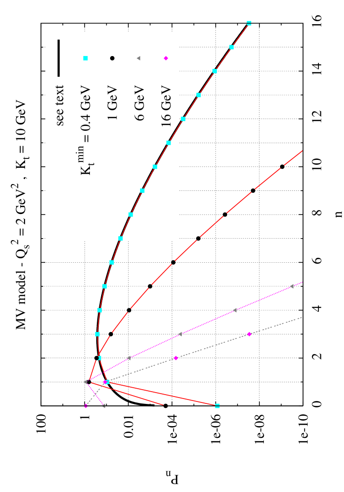
Figure 2: Distribution of the probabilities $P_{n}$ in the MV model. The produced particle has acquired a transverse momentum $k_{\perp}=10$ GeV and the saturation momentum is set to the value $Q_{s}^{2}=2$ GeV². The threshold $k_{\perp}^{\rm min}$ for counting the recoiling particles takes values between $0.4$ and $16$ GeV. The black solid line represents the result of an approximate calculation (see text).

One can see that the width of the multiplicity distribution decreases with an increasing $k_{\perp}^{\rm min}$. This is of course quite natural, since by increasing $k_{\perp}^{\rm min}$ it becomes less and less likely to have events in which there are a large number of recoils. Note also that for all $k_{\perp}^{\rm min}$ such that $Q_{s}\ll k_{\perp}^{\rm min}\lesssim k_{\perp}$, the most likely number of recoils is $n=1$, while for $k_{\perp}<k_{\perp}^{\rm min}$ the most likely situation is $n=0$.

We can in fact understand analytically this distribution $P_{n}$ in the situation where the momentum exchange $k_{\perp}$ between the incoming gluon and the nucleus is much larger than the other scales, $Q_{s},k_{\perp}^{\rm min}\ll k_{\perp}$. This means that we need only to estimate the functions $A$ and $B$ defined in Eq. (9) for values of $x_{\perp}$ that are much smaller than the inverse saturation momentum, $x_{\perp}\ll Q_{s}^{-1}$, and much smaller than $(k_{\perp}^{\rm min})^{-1}$. This allows us to expand the exponential $\exp(i{\boldsymbol{l}}_{\perp}\cdot{\boldsymbol{x}}_{\perp})$ in order to evaluate the integral over ${\boldsymbol{l}}_{\perp}$, leading to the following approximations:

$$A(x_{\perp})\approx-\frac{g^{4}N_{c}}{16\pi}\,x_{\perp}^{2}\,\ln\left(\frac{1}{\Lambda x_{\perp}}\right)\;,$$

$$B({\boldsymbol{x}}_{\perp}|k_{\perp}^{\rm min})\approx\frac{g^{4}N_{c}}{8\pi}\left[\frac{1}{k_{\perp}^{\rm min\ 2}}-\frac{x_{\perp}^{2}}{2}\,\ln\left(\frac{1}{k_{\perp}^{\rm min}x_{\perp}}\right)\right]\;.$$ (15)

Then, in order to evaluate the generating function via Eqs. (10) and (11), one can use the following result, valid at large $k_{\perp}$,

$$\int d^{2}{\boldsymbol{x}}_{\perp}\;e^{-i{\boldsymbol{k}}_{\perp}\cdot{\boldsymbol{x}}_{\perp}}\;e^{-Cx_{\perp}^{2}\ln(x_{\perp}^{0}/x_{\perp})}\approx\frac{8\pi C}{k_{\perp}^{4}}\;.$$ (16)

(The value of the constant $x^{0}_{\perp}$ has no influence on this result in the limit of large $k_{\perp}$.) Thanks to this formula, we obtain immediately

$$F(z,k_{\perp}|k_{\perp}^{\rm min})\approx z\;e^{\frac{g^{4}N_{c}\mu_{0}^{2}}{8\pi(k_{\perp}^{\rm min})^{2}}(z-1)}\;.$$ (17)

One can see that in this limit, the generating function is universal in the sense that it does not depend on the momentum $k_{\perp}$ acquired by the incoming gluon. Moreover, the probability of having zero scatterings with a recoil above $k_{\perp}^{\rm min}$, $P_{0}=F(z=0,k_{\perp}|k_{\perp}^{\rm min})$, is zero. In other words, when $k_{\perp}^{\rm min}\ll k_{\perp}$, there must be at least one scattering above $k_{\perp}^{\rm min}$ in order to give such a large $k_{\perp}$ to the incoming gluon.

We can go a bit further, since it is easy to recognize that the generating function obtained in Eq. (17) corresponds to the following distribution of probabilities:

$$P_{0}=0\;,$$

$$P_{n}=\frac{\overline{n}^{\,n-1}}{(n-1)!}\;e^{-\overline{n}}\quad\mbox{with\ \ }\overline{n}\equiv\frac{g^{4}N_{c}\mu_{0}^{2}}{8\pi(k_{\perp}^{\rm min})^{2}}\;.$$ (18)

In other words, the distribution of multiplicities is a Poisson distribution shifted by one unit. The physical meaning of this shift will become transparent later in the discussion. In Figure 2, we have compared for $k_{\perp}^{\rm min}=0.4$ GeV the numerically evaluated $P_{n}$’s with such a shifted Poisson distribution, and as one can see the two agree extremely well (except for $P_{0}$, which is very small but not exactly zero).

Note however that the value of $\overline{n}$ we had to use in this fit differs by about 25% from the predicted value given in Eq. (18). This kind of deviation is expected, because this formula for $\overline{n}$ is only valid for $k_{\perp}^{\rm min}\gg\Lambda$, a condition which is at best marginally satisfied for $k_{\perp}^{\rm min}=0.4~{}$GeV (we have taken the infrared cutoff to be $\Lambda=0.2~{}$GeV). Moreover, from the approximations that have been used in order to obtain Eq. (15), a generating function of the form $F(z)=z\;\exp(\overline{n}(z-1))$ – that leads to a shifted Poisson distribution – is obtained as long as $k_{\perp}\gg Q_{s},k_{\perp}^{\rm min}$. It is only the accurate prediction of the value of $\overline{n}$ that requires in addition $k_{\perp}^{\rm min}\gg\Lambda$. This explains why, despite the fact that $\overline{n}$ was not very accurately predicted at $k_{\perp}^{\rm min}=0.4~{}$GeV, the obtained distribution was nevertheless of the form given in Eq. (18) with a very good accuracy, because $k_{\perp}=10~{}$GeV.

4.2 Number of recoils

Figure 3: Number of recoiling scattering centers in the MV model, as a function of the threshold $k_{\perp}^{\rm min}$. The saturation momentum is set to the value $Q_{s}^{2}=2$ GeV², and the momentum $k_{\perp}$ of the produced particle is varied between $1$ and $50$ GeV.

Next, we display in Figure 3 the average number of recoils above the threshold $k_{\perp}^{\rm min}$, defined as

$$N(k_{\perp}|k_{\perp}^{\rm min})\equiv\sum_{n=1}^{\infty}n\,P_{n}(k_{\perp}|k_{\perp}^{\rm min})\;,$$ (19)

as a function of $k_{\perp}^{\rm min}$, for various momenta $k_{\perp}$ and a fixed $Q_{s}^{2}=2$ GeV². We see that the number of recoils grows significantly at small $k_{\perp}^{\rm min}$, and tends in this region to become universal and independent of $k_{\perp}$. Moreover, a striking feature of this number of recoils is that it is very close to unity for any value of $k_{\perp}^{\rm min}$ such that $Q_{s}\ll k_{\perp}^{\rm min}\lesssim k_{\perp}$. This means that when the gluon acquires a large momentum $k_{\perp}$ from the nucleus, there is always one hard recoil – and only one – that provides most of this large momentum.

Again, it is possible to have an analytic understanding of these properties of the average number of recoils from Eq. (17). Indeed, the average number of recoils is given by the derivative of the generating function at $z=1$, and we obtain

$$N(k_{\perp}|k_{\perp}^{\rm min})\approx 1+\frac{g^{4}N_{c}\mu_{0}^{2}}{8\pi(k_{\perp}^{\rm min})^{2}}\;.$$ (20)

This analytic expression is also displayed in Figure 3, and it reproduces well the numerical calculation for $k_{\perp}^{\rm min}\lesssim k_{\perp}$. It deviates from it at very small $k_{\perp}^{\rm min}$ due to a non-trivial interplay between $k_{\perp}^{\rm min}$ and the infrared cutoff $\Lambda$, which is not correctly captured by our simple analytic calculation. And of course this analytical result does not work for $k_{\perp}^{\rm min}\geq k_{\perp}$ because this is outside the range of validity of our approximations.

4.3 Momentum distribution of the recoils

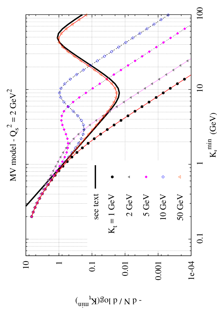
Figure 4: Distribution of the number of recoiling scattering centers in the MV model, as a function of the threshold $k_{\perp}^{\rm min}$. The saturation momentum is set to the value $Q_{s}^{2}=2$ GeV², and the momentum $k_{\perp}$ of the produced particle is varied between $1$ and $50$ GeV.

In Figure 4, we have taken the derivative of the average number of recoils with respect to $k_{\perp}^{\rm min}$, in order to obtain the momentum distribution of these recoils. At large $k_{\perp}$, one can clearly see that this distribution consists of two components: a universal (almost independent of $k_{\perp}$) semi-hard component made of recoils with momenta of the order of $Q_{s}$ or smaller, and a component peaked around $k_{\perp}^{\rm min}=k_{\perp}$. The latter peak has an area unity, and it is simply translated when $k_{\perp}$ is changed. By taking the derivative of Eq. (20), one can readily obtain a contribution that reproduces well the numerical result in the semi-hard region

$$-\frac{dN}{d\ln(k_{\perp}^{\rm min})}\approx\frac{g^{4}N_{c}\mu_{0}^{2}}{4\pi(k_{\perp}^{\rm min})^{2}}\;.$$ (21)

In fact, it turns out that it is also possible to estimate this derivative in the region where $k_{\perp}^{\rm min}$ is comparable to or larger than $k_{\perp}$ (both of them being very large compared to $Q_{s}$). When both $k_{\perp}^{\rm min}$ and $k_{\perp}$ are large compared to $Q_{s}$ (i.e. to $\mu_{0}^{2}$), it is enough to expand the exponentials of $A$ and $B$ in Eq. (11) to first order, and write

$$F(z,k_{\perp}|k_{\perp}^{\rm min})\approx\frac{\int d^{2}{\boldsymbol{x}}_{\perp}\;e^{-i{\boldsymbol{k}}_{\perp}\cdot{\boldsymbol{x}}_{\perp}}\;\Big{[}A(x_{\perp})+(z-1)B(x_{\perp}|k_{\perp}^{\rm min})\Big{]}}{\int d^{2}{\boldsymbol{x}}_{\perp}\;e^{-i{\boldsymbol{k}}_{\perp}\cdot{\boldsymbol{x}}_{\perp}}\;A(x_{\perp})}\;.$$ (22)

The multiplicity being the derivative of $F$ at $z=1$, we have

$$N(k_{\perp}|k_{\perp}^{\rm min})\approx\frac{\int d^{2}{\boldsymbol{x}}_{\perp}\;e^{-i{\boldsymbol{k}}_{\perp}\cdot{\boldsymbol{x}}_{\perp}}\;B(x_{\perp}|k_{\perp}^{\rm min})}{\int d^{2}{\boldsymbol{x}}_{\perp}\;e^{-i{\boldsymbol{k}}_{\perp}\cdot{\boldsymbol{x}}_{\perp}}\;A(x_{\perp})}\;.$$ (23)

Going back to the form (9) of $A$ and $B$, we see that the integration over ${\boldsymbol{x}}_{\perp}$ simply produces a $\delta({\boldsymbol{k}}_{\perp}-{\boldsymbol{l}}_{\perp})$, making the integral over ${\boldsymbol{l}}_{\perp}$ trivial as well. In this kinematical region, we obtain an extremely simple result:

$$N(k_{\perp}|k_{\perp}^{\rm min})\approx\frac{\sigma({\boldsymbol{k}}_{\perp})\vartheta(k_{\perp}/k_{\perp}^{\rm min})}{\sigma({\boldsymbol{k}}_{\perp})}=\vartheta(k_{\perp}/k_{\perp}^{\rm min})\;.$$ (24)

We see that this component of the multiplicity is nothing but the cutoff function that we are using in order to separate the momenta that are below $k_{\perp}^{\rm min}$ from those that are above. Therefore, the precise shape of the average number of scatterings for $k_{\perp}^{\rm min}$ above $k_{\perp}$ is not a property of QCD, but merely reflects the fact that we have an extended rather than a sharp cutoff. Nevertheless, the interpretation of this contribution is quite straightforward: when $k_{\perp}^{\rm min}$ is smaller than $k_{\perp}$ there is one recoil (that absorbs most of the momentum $k_{\perp}$), but it is unlikely that there is a recoil with a momentum bigger than the momentum $k_{\perp}$. Taking a derivative with respect to $k_{\perp}^{\rm min}$, we obtain the corresponding contribution to the momentum distribution of the recoils:

$$-\frac{dN}{d\ln(k_{\perp}^{\rm min})}\approx\frac{k_{\perp}}{k_{\perp}^{\rm min}}\;\vartheta^{\prime}(k_{\perp}/k_{\perp}^{\rm min})\;.$$ (25)

In Figure 4, we have represented for $k_{\perp}=50$ GeV the sum of the contributions given in Eqs. (21) and (25) (taking for the latter the same “step function” $\vartheta(x)$ as the one used in the numerical calculation of the integral $B$). The sum of these two components reproduces with a fairly good accuracy the numerical results for all $k_{\perp}^{\rm min}$ down to $k_{\perp}^{\rm min}\sim 500$ MeV. The small discrepancy between our analytical estimate of the peaked contribution and its numerical value is due to rescattering corrections – indeed, our derivation of Eq. (25) retains only the leading-twist contribution. As one can see, the numerically obtained peak is slightly shifted to the left of the analytical result. This is easy to understand: since there are a few semi-hard scatterings in addition to the hard one, the hard scattering needs to provide a little less than the momentum $k_{\perp}$ acquired by the gluon. This shift is a form of collisional energy loss (for a cold nuclear medium).

Note that, when the “step function” $\vartheta(x)$ becomes a real step function $\theta(x)$, Eq. (25) would imply a peak proportional to $\delta(k_{\perp}^{\rm min}-k_{\perp})$. However, we expect that higher-twist corrections to Eq. (22) would be important in this limit, and they are likely to smear out slightly the delta peak.

Before considering the $Q_{s}$ dependence, let us come back to the Poisson distribution shifted by one unit found in Eq. (18), when $k_{\perp}^{\rm min}\ll k_{\perp}$. The shift by one unit is due to the fact that, when the threshold $k_{\perp}^{\rm min}$ is so low compared to $k_{\perp}$, there is always at least one scattering (moreover, we know now that this scattering has a recoil momentum which is close to $k_{\perp}$). The meaning of Eq. (18) is therefore that the remaining $n-1$ – semi-hard – scatterings that come along with this hard scattering have a Poissonian distribution, which merely reflects the fact that they are independent from one another.

4.4 Dependence on $Q_{s}$

Finally, let us have a look at the dependence on the saturation momentum. For this, we set the momentum $k_{\perp}$ acquired by the gluon to $10$ GeV, and we study the momentum distribution of the recoils for various values of $Q_{s}^{2}$. The results of this analysis are displayed in Figure 5.

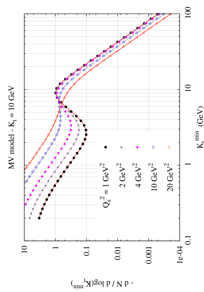
Figure 5: $Q_{s}$ dependence of the distribution of the number of recoiling scattering centers in the MV model. The saturation momentum is varied between $Q_{s}^{2}=1$ GeV² and $Q_{s}^{2}=20$ GeV², and the momentum $k_{\perp}$ of the produced particle is set to $10$ GeV.

As long as the saturation scale $Q_{s}$ remains small compared to $k_{\perp}$, only the semi-hard part of the distribution is affected by changes of $Q_{s}$, while the peak around $k_{\perp}^{\rm min}=k_{\perp}$ remains unchanged. The latter result is due to the fact that, since this peak is well approximated by a leading-twist calculation, it must be independent of saturation physics with the same accuracy. It is only when $Q_{s}$ becomes very large that one cannot neglect higher-twist corrections at large $k_{\perp}^{\rm min}$, and that the peak at $k_{\perp}^{\rm min}=k_{\perp}$ eventually disappears. Since the distribution of semi-hard recoils is quite sensitive to the value of $Q_{s}$ (it is proportional to $g^{4}\mu_{0}^{2}$, which is proportional to $Q_{s}^{2}$ up to a logarithm), it could perhaps be used as a way to estimate $Q_{s}$.

The disappearance of the peak also provides a qualitative answer to our initial question regarding the possible existence of monojets: any parton produced with a $k_{\perp}$ which is much larger than the saturation momentum in the nucleus must have its momentum balanced by another parton on the opposite side (the latter comes from the scattering center that has undergone the hard collision). But all the partons with a transverse momentum comparable to or smaller than $Q_{s}$ need not have their momentum balanced by a leading parton on the opposite side, since it can be balanced by several softer particles (coming from the semi-hard component of the distribution of recoils). As long as the saturation momentum remains relatively small, say $Q_{s}\sim 1-3$ GeV, this conclusion is not going to alter one’s common expectations regarding jets: all hard jets with a momentum larger than say $10$ GeV must come in pairs. It is only for a very large $Q_{s}$ that one would start seeing non-conventional event topologies where a hard jet would have its momentum balanced by a large number of softer particles.

5 Effect of leading-twist shadowing

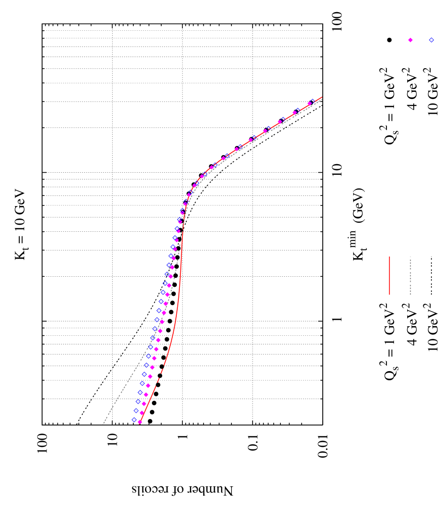
Figure 6: $Q_{s}$ dependence of the number of recoiling scattering centers in the asymptotic model, compared to the MV model. The saturation momentum is varied between $Q_{s}^{2}=1$ GeV² and $Q_{s}^{2}=10$ GeV², and the momentum $k_{\perp}$ of the produced particle is set to $10$ GeV. Lines: MV model. Dots: asymptotic model.

Let us now briefly compare the results previously obtained using the MV model, with those one obtains by using the model defined by Eq. (14). Basically, the two models – at an identical $Q_{s}$ – differ by the nature of the correlations among the color charges in the nucleus. In particular, the MV model does not have any leading-twist shadowing, while the second model has an anomalous dimension $\gamma$ different from unity and thus provides some shadowing. It is believed that the latter model is a better description of a nucleus at very small momentum fractions $x$.

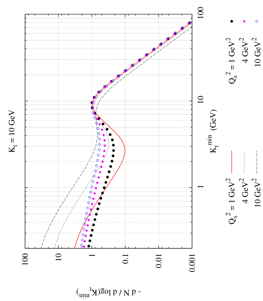
Figure 7: $Q_{s}$ dependence of the distribution of the number of recoiling scattering centers in the asymptotic model, compared to the MV model. The saturation momentum is varied between $Q_{s}^{2}=1$ GeV² and $Q_{s}^{2}=10$ GeV², and the momentum $k_{\perp}$ of the produced particle is set to $10$ GeV. Lines: MV model. Dots: asymptotic model.

In Figure 6, we first compare the average number of recoils for the two models (thin lines: MV model – dots: asymptotic model). The value of the “trigger momentum” $k_{\perp}$ is held fixed at a value of $10$ GeV, and the saturation momentum squared is varied in the range $1-10$ GeV². One sees that the number of semi-hard and soft recoils is quite smaller in the asymptotic model than in the MV model. At the largest of the considered $Q_{s}$, the number of soft recoils is ten times smaller in the asymptotic model than in the MV model. We interpret this as an effect of shadowing, which “hides” the scattering centers from the passing gluon. A similar observation was made in [36], where it was seen that the multiple scatterings that lead to the Cronin effect are almost inexistent in this asymptotic model. Also, an effect of shadowing is that the dependence on $Q_{s}$ is much weaker in the asymptotic model: piling up more and more color charges in the nucleus does not lead to many more scatterings if the gluon cannot see them because of shadowing. This weaker dependence on $Q_{s}$ is also seen at large $k_{\perp}^{\rm min}$, where one can hardly see any change even at $Q_{s}^{2}=10$ GeV².

Another feature of the asymptotic model is that the “plateau” at $N=1$ for $Q_{s}\ll k_{\perp}^{\rm min}\lesssim k_{\perp}$ is no longer really flat. Instead of a wide plateau between $Q_{s}$ and $k_{\perp}$, one has instead a slow but steady rise of the multiplicity as $k_{\perp}^{\rm min}$ decreases. For this reason, we expect the two-component structure of the momentum distribution of the recoils to be less pronounced in the asymptotic model than in the MV model. This is what we check by taking a derivative with respect to $k_{\perp}^{\rm min}$, as illustrated in Figure 7. In these plots, one can see that the dip between the low-momentum component and the peak around $k_{\perp}^{\rm min}=k_{\perp}$ is not as deep as in the MV model. This means that one should expect the distribution of momenta in the “away-side jet” to be more extended towards softer momenta, as one probes the nucleus at smaller and smaller values of $x$.

6 Measuring the impact parameter
from the multiplicity?

Based on the above study, one can address a related question: is there a correlation between the measured multiplicity in a pA collision (event by event) and the impact parameter of the collision? and with what accuracy could one determine the impact parameter based on this correlation?

In this theoretical study, the question one can answer is the following: if the measured multiplicity in an event is $n$ (in addition to the hard jet of momentum $k_{\perp}$), what is the probability distribution of the various impact parameters? In order to answer this question, we will make three assumptions:

• When two bunches of nuclei and protons collide in an accelerator, all the impact parameters ${\boldsymbol{b}}$ are equally probable.

• The only recorded events are those where $\big{|}{\boldsymbol{b}}\big{|}\leq R$, where $R$ is the radius of the nucleus (we neglect the radius of the proton). Assuming here for simplicity that the trigger efficiency is the same for all ${\boldsymbol{b}}$’s, the probability of a given impact parameter (in the absence of any other information about the collision) is a priori equal to $P({\boldsymbol{b}})=1/\pi R^{2}\;.$

• The density parameter $\mu_{0}^{2}$ at a given impact parameter $b$ is proportional to the thickness of the nucleus at this impact parameter, i.e. to $\sqrt{R^{2}-b^{2}}\;.$

Let us introduce the probability ${\cal P}(n,{\boldsymbol{b}})$ of having simultaneously the impact parameter ${\boldsymbol{b}}$ and the multiplicity $n$ (it is implicit in all this section that we mean the multiplicity above a certain threshold $k_{\perp}^{\rm min}$ when the passing gluon has acquired the momentum $k_{\perp}$ – these variables will not be written anymore in order to avoid encumbering the notations). ${\cal P}(n,{\boldsymbol{b}})$ must be normalized so that one has

$$\sum_{n=0}^{\infty}\int d^{2}{\boldsymbol{b}}\;{\cal P}(n,{\boldsymbol{b}})=1\;.$$ (26)

The probabilities $P_{n}$ defined earlier in this paper can be obtained from this more general object by

$$P_{n}=\frac{{\cal P}(n,{\boldsymbol{b}})}{\sum_{n}\;{\cal P}(n,{\boldsymbol{b}})}\;.$$ (27)

The denominator is necessary so that the $P_{n}$’s add up to unity. Obviously, this denominator is a function that depends only on ${\boldsymbol{b}}$, whose integral over ${\boldsymbol{b}}$ is unity. It is nothing but the probability of having a collision with impact parameter ${\boldsymbol{b}}$, when the incoming gluon has been scattered off the nucleus with a momentum ${\boldsymbol{k}}_{\perp}$. It is easy to convince oneself that this probability is given by:

$$\sum_{n}\;{\cal P}(n,{\boldsymbol{b}})=\frac{C({\boldsymbol{k}}_{\perp})}{\int d^{2}{\boldsymbol{b}}\;C({\boldsymbol{k}}_{\perp})}\;,$$ (28)

where the ${\boldsymbol{b}}$ dependence of $C({\boldsymbol{k}}_{\perp})$ comes implicitly via the parameter $\mu_{0}^{2}$. If there were no trigger bias, this quantity would simply be uniform and equal to $(\pi R^{2})^{-1}$. However, because it is slightly more likely to have a large ${\boldsymbol{k}}_{\perp}$ in central collisions than in peripheral ones, the mere fact of selecting a specific ${\boldsymbol{k}}_{\perp}$ in the final state introduces a certain bias in the distribution of impact parameters. Therefore, one has

$${\cal P}(n,{\boldsymbol{b}})=\frac{P_{n}\,C({\boldsymbol{k}}_{\perp})}{\int d^{2}{\boldsymbol{b}}\;C({\boldsymbol{k}}_{\perp})}\;,$$ (29)

and we see that no new calculation is necessary. It will be sufficient to calculate $P_{n}$ at fixed $n$ as a function of ${\boldsymbol{b}}$ (the $b$ dependence comes in via $\mu_{0}^{2}\sim\sqrt{R^{2}-b^{2}}$).

From this object ${\cal P}(n,{\boldsymbol{b}})$, it is easy to obtain the normalized distribution of impact parameters conditional to having an event with the multiplicity $n$, which is the solution to the question we asked,

$$p_{n}({\boldsymbol{b}})=\frac{{\cal P}(n,{\boldsymbol{b}})}{\int d^{2}{\boldsymbol{b}}\;{\cal P}(n,{\boldsymbol{b}})}\;.$$ (30)

We have evaluated this quantity numerically in the MV model. The only extra parameters that need to be set are the coefficient of proportionality between the density $\mu_{0}^{2}$ and the size $\sqrt{R^{2}-b^{2}}$ – we set it so that the saturation scale at the center of the nucleus ($b=0$) is $2$ GeV² – and the nuclear radius, taken to be $R=6$ fm. The results are displayed in Figure 8, for events where the gluon acquires the momentum $k_{\perp}=10$ GeV and with a threshold momentum of $k_{\perp}^{\rm min}=0.4$ GeV for counting the number of recoils.

Figure 8: Probability distribution of the impact parameter for various final multiplicities, in the MV model. The trigger momentum is set to $k_{\perp}=10$ GeV, the threshold momentum to $k_{\perp}^{\rm min}=0.4$ GeV.

The results are fairly intuitive: events with a low multiplicity are dominated by large impact parameters, and events with a high multiplicity are much more central. But we also see that selecting a given final multiplicity only gives a fairly vague idea of the impact parameter, since the distributions of probability for $b$ at a fixed $n$ are quite wide, with important overlaps between the curves for different final multiplicities. And to make things even more difficult, the two extreme values of the final multiplicity ($n=1$ and $n=16$ in our example), which have the least overlap in $b$, correspond to very rare events as one can judge from the figure 2. Therefore, it seems realistic to make two centrality classes, reasonably well separated in impact parameter, based on the observed number of recoils. Changing the value of the threshold $k_{\perp}^{\rm min}$ may help this separation, but we have not investigated that approach systematically here.

7 Conclusions

In this paper, we have calculated the distribution of the number of scatterings in proton-nucleus collisions, in the Color Glass Condensate framework. This has been done by calculating the generating function for the probabilities of having a definite number of scatterings. We observe that, when the produced gluon has a transverse momentum which is large compared to the saturation scale, then this momentum is provided mostly by a single scattering center in the nucleus, leading therefore to the familiar di-jet configuration. This hard scattering is accompanied by a larger number of semi-hard scatterings, with transferred momenta of the order of the saturation momentum or smaller. By comparing the McLerran-Venugopalan model with a model that describes the regime of very small $x$, we also see that the shadowing present in the latter tends to suppress these semi-hard scatterings, and to blur the separation between the hard and semi-hard scatterings. Finally, we have discussed the correlation between the final multiplicity and the impact parameter, and shown that it is not a very strong correlation, that can at best be used to make a gross separation in at most 2-3 centrality bins.

As a final note, let us mention that the results discussed in this paper are a particular case of some general results on random walks (in two dimensions in our case) where at each step one may have a random step size (both in magnitude and direction), according to a certain probability law. If this probability distribution for the step sizes is falling very quickly, then the only way that the random walk may end far away from the origin is to add up a very large number of small steps. On the contrary, if this probability distribution has an extended tail at large step sizes, such that the variance is infinite – such random walks are known as “Lévy flights” – then the most efficient way to go far from the origin is to make one big step, accompanied by smaller steps. Note that the distance from the origin reached after a large number of steps has very different distributions in these two situations: Gaussian in the first case, as opposed to a power-law tail in the second case. The interested reader may see [54], pp. 42-59, for a pedagogical introduction to Lévy statistics.

In the problem of independent multiple scatterings that we have discussed in this paper, the “step size” is the transverse momentum acquired by the gluon at each scattering, which has a probability distribution that falls like $\sigma({\boldsymbol{l}}_{\perp})\sim{\boldsymbol{l}}_{\perp}^{-4}$ in the MV model (even slower if there is an anomalous dimension different from unity). The variance of the step sizes, $\int d^{2}{\boldsymbol{l}}_{\perp}\;l_{\perp}^{2}\;\sigma({\boldsymbol{l}}_{\perp})$, is thus infinite, and our problem falls in the category of Lévy flights. Many of our results can be understood from this analogy.

References

- [1] L.V. Gribov, E.M. Levin, M.G. Ryskin, Phys. Rept. 100, 1 (1983).
- [2] A.H. Mueller, J-W. Qiu, Nucl. Phys. B 268, 427 (1986).
- [3] J.P. Blaizot, A.H. Mueller, Nucl. Phys. B 289, 847 (1987).
- [4] I. Balitsky, L.N. Lipatov, Sov. J. Nucl. Phys. 28, 822 (1978).
- [5] E.A. Kuraev, L.N. Lipatov, V.S. Fadin, Sov. Phys. JETP 45, 199 (1977).
- [6] L.D. McLerran, R. Venugopalan, Phys. Rev. D 49, 2233 (1994).
- [7] L.D. McLerran, R. Venugopalan, Phys. Rev. D 49, 3352 (1994).
- [8] L.D. McLerran, R. Venugopalan, Phys. Rev. D 50, 2225 (1994).
- [9] S. Jeon, R. Venugopalan, Phys. Rev. D 70, 105012 (2004).
- [10] E. Iancu, A. Leonidov, L.D. McLerran, Nucl. Phys. A 692, 583 (2001).
- [11] E. Iancu, A. Leonidov, L.D. McLerran, Phys. Lett. B 510, 133 (2001).
- [12] E. Ferreiro, E. Iancu, A. Leonidov, L.D. McLerran, Nucl. Phys. A 703, 489 (2002).
- [13] J. Jalilian-Marian, A. Kovner, A. Leonidov, H. Weigert, Nucl. Phys. B 504, 415 (1997).
- [14] J. Jalilian-Marian, A. Kovner, A. Leonidov, H. Weigert, Phys. Rev. D 59, 014014 (1999).
- [15] J. Jalilian-Marian, A. Kovner, A. Leonidov, H. Weigert, Phys. Rev. D 59, 034007 (1999).
- [16] J. Jalilian-Marian, A. Kovner, A. Leonidov, H. Weigert, Erratum. Phys. Rev. D 59, 099903 (1999).
- [17] A. Kovner, G. Milhano, Phys. Rev. D 61, 014012 (2000).
- [18] A. Kovner, G. Milhano, H. Weigert, Phys. Rev. D 62, 114005 (2000).
- [19] J. Jalilian-Marian, A. Kovner, L.D. McLerran, H. Weigert, Phys. Rev. D 55, 5414 (1997).
- [20] I. Balitsky, Nucl. Phys. B 463, 99 (1996).
- [21] Yu.V. Kovchegov, Phys. Rev. D 61, 074018 (2000).
- [22] A. Krasnitz, R. Venugopalan, Phys. Rev. Lett. 84, 4309 (2000).
- [23] A. Krasnitz, R. Venugopalan, Phys. Rev. Lett. 86, 1717 (2001).
- [24] A. Krasnitz, Y. Nara, R. Venugopalan, Nucl. Phys. A 727, 427 (2003).
- [25] A. Krasnitz, Y. Nara, R. Venugopalan, Phys. Rev. Lett. 87, 192302 (2001).
- [26] T. Lappi, Phys. Rev. C 67, 054903 (2003).
- [27] P. Romatschke, R. Venugopalan, Phys. Rev. Lett. 96, 062302 (2006).
- [28] P. Romatschke, R. Venugopalan, hep-ph/0510292.
- [29] Yu.V. Kovchegov, A.H. Mueller, Nucl. Phys. B 529, 451 (1998).
- [30] A. Kovner, U. Wiedemann, Phys. Rev. D 64, 114002 (2001).
- [31] Yu.V. Kovchegov, K. Tuchin, Phys. Rev. D 65, 074026 (2002).
- [32] A. Dumitru, L.D. McLerran, Nucl. Phys. A 700, 492 (2002).
- [33] A. Dumitru, J. Jalilian-Marian, Phys. Rev. Lett. 89, 022301 (2002).
- [34] A. Dumitru, J. Jalilian-Marian, Phys. Lett. B 547, 15 (2002).
- [35] F. Gelis, J. Jalilian-Marian, Phys. Rev. D 67, 074019 (2003).
- [36] J.P. Blaizot, F. Gelis, R. Venugopalan, Nucl. Phys. A 743, 13 (2004).
- [37] F. Gelis, Y. Methar-Tani, Phys. Rev. D 73, 034019 (2006).
- [38] N.N. Nikolaev, W. Schafer, Phys. Rev. D 71, 014023 (2005).
- [39] F. Gelis, R. Venugopalan, Phys. Rev. D 69, 014019 (2004).
- [40] K. Tuchin, Phys. Lett. B 593, 66 (2004).
- [41] J.P. Blaizot, F. Gelis, R. Venugopalan, Nucl. Phys. A 743, 57 (2004).
- [42] J. Jalilian-Marian, Y. Kovchegov, Phys. Rev. D 70, 114017 (2004), Erratum-ibid. D 71, 079901 (2005).
- [43] N.N. Nikolaev, W. Schafer, B.G. Zakharov, Phys. Rev. Lett. 95, 221803 (2005).
- [44] N.N. Nikolaev, W. Schafer, B.G. Zakharov, Phys. Rev. D 72, 114018 (2005).
- [45] N.N. Nikolaev, W. Schafer, B.G. Zakharov, Phys. Rev. D 72, 034033 (2005).
- [46] H. Fujii, F. Gelis, R. Venugopalan, Phys. Rev. Lett. 95, 162002 (2005).
- [47] R. Baier, A. Kovner, M. Nardi, U.A. Wiedemann, Phys. Rev. D 72, 094013 (2005).
- [48] H. Fujii, F. Gelis, R. Venugopalan, hep-ph/0603099.
- [49] J. Jalilian-Marian, Y. Kovchegov, Prog. Part. Nucl. Phys. 56, 104 (2006).
- [50] D. Kharzeev, E. Levin, L.D. McLerran, Nucl. Phys. A 748, 627 (2005).
- [51] J. Adams, et al., (STAR Collaboration) Phys. Rev. Lett. 91, 072304 (2003).
- [52] F. Gelis, A. Peshier, Nucl. Phys. A 697, 879 (2002).
- [53] E. Iancu, K. Itakura, L.D. McLerran, Nucl. Phys. A 724, 181 (2003).
- [54] F. Bardou, J-P. Bouchaud, A. Aspect, C. Cohen-Tannoudji, Lévy statistics and laser cooling, Cambridge University Press (2002).