Nearly Tri-bimaximal Neutrino Mixing and CP Violation
from $\mu$-$\tau$ Symmetry Breaking

Abstract

Assuming the Majorana nature of massive neutrinos, we generalize the Friedberg-Lee neutrino mass model to include CP violation in the neutrino mass matrix $M_{\nu}$. We show that a favorable neutrino mixing pattern (with $\theta_{12}\approx 35.3^{\circ}$, $\theta_{23}=45^{\circ}$, $\theta_{13}\neq 0^{\circ}$ and $\delta=90^{\circ}$) can naturally be derived from $M_{\nu}$, if it has an approximate or softly-broken $\mu$-$\tau$ symmetry. We point out a different way to obtain the nearly tri-bimaximal neutrino mixing with $\delta=0^{\circ}$ and non-vanishing Majorana phases. The most general case, in which all the free parameters of $M_{\nu}$ are complex and the resultant neutrino mixing matrix contains both Dirac and Majorana phases of CP violation, is also discussed.

I Introduction

The solar [1], atmospheric [2], reactor [3] and accelerator [4] neutrino experiments have provided us with very convincing evidence that neutrinos are massive and lepton flavors are mixed. Given the basis in which the flavor eigenstates of charged leptons are identified with their mass eigenstates, the phenomenon of neutrino mixing can simply be described by a $3\times 3$ unitary matrix $V$ which transforms the neutrino mass eigenstates $(\nu_{1},\nu_{2},\nu_{3})$ into the neutrino flavor eigenstates $(\nu_{e},\nu_{\mu},\nu_{\tau})$. We assume massive neutrinos to be Majorana particles and parametrize $V$ as

$$V=\left(\matrix{c_{12}c_{13}&s_{12}c_{13}&s_{13}e^{-i\delta}\cr-s_{12}c_{23}-c_{12}s_{23}s_{13}e^{i\delta}&c_{12}c_{23}-s_{12}s_{23}s_{13}e^{i\delta}&s_{23}c_{13}\cr s_{12}s_{23}-c_{12}c_{23}s_{13}e^{i\delta}&-c_{12}s_{23}-s_{12}c_{23}s_{13}e^{i\delta}&c_{23}c_{13}}\right)\left(\matrix{e^{i\rho}&0&0\cr 0&e^{i\sigma}&0\cr 0&0&1\cr}\right)\;,$$ (1)

where $c_{ij}\equiv\cos\theta_{ij}$ and $s_{ij}\equiv\sin\theta_{ij}$ (for $ij=12,23$ and $13$). A global analysis of current experimental data [5] yields $30^{\circ}<\theta_{12}<38^{\circ}$, $36^{\circ}<\theta_{23}<54^{\circ}$ and $\theta_{13}<10^{\circ}$ at the $99\%$ confidence level, but three CP-violating phases of $V$ (i.e., the Dirac phase $\delta$ and the Majorana phases $\rho$ and $\sigma$) are entirely unrestricted. In order to interpret the largeness of two neutrino mixing angles together with the smallness of three neutrino masses, many theoretical and phenomenological models of lepton mass matrices have been proposed in the literature [6]. Among them, the scenarios based on possible flavor symmetries are particularly simple, suggestive and predictive.

In this paper, we focus our interest on the neutrino mass model proposed recently by Friedberg and Lee (FL) [7]. The neutrino mass operator in the FL model is simply given by

$${\cal L}_{\nu-\rm mass} = a\left(\overline{\nu}_{\tau}-\overline{\nu}_{\mu}\right)\left(\nu_{\tau}-\nu_{\mu}\right)+b\left(\overline{\nu}_{\mu}-\overline{\nu}_{e}\right)\left(\nu_{\mu}-\nu_{e}\right)+c\left(\overline{\nu}_{e}-\overline{\nu}_{\tau}\right)\left(\nu_{e}-\nu_{\tau}\right)~{}~{}~{}~{}~{}~{}~{}$$ (3)

$$+m_{0}\left(\overline{\nu}_{e}\nu_{e}+\overline{\nu}_{\mu}\nu_{\mu}+\overline{\nu}_{\tau}\nu_{\tau}\right)\;,$$

where $a$, $b$, $c$ and $m_{0}$ are all assumed to be real. A salient feature of ${\cal L}_{\nu-\rm mass}$ is its partial gauge-like symmetry; i.e., its $a$, $b$ and $c$ terms are invariant under the transformation $\nu_{\alpha}\rightarrow\nu_{\alpha}+z$ (for $\alpha=e,\mu,\tau$) with $z$ being a space-time independent constant element of the Grassmann algebra [7]. Eq. (2) means that the neutrino mass matrix $M_{\nu}$ takes the form

$$M_{\nu}\;=\;m_{0}\left(\matrix{1&0&0\cr 0&1&0\cr 0&0&1\cr}\right)~{}+~{}\left(\matrix{b+c&-b&-c\cr-b&a+b&-a\cr-c&-a&a+c\cr}\right)\;.$$ (4)

Diagonalizing $M_{\nu}$ by the transformation $V^{\dagger}_{\rm FL}M_{\nu}V^{*}_{\rm FL}={\rm Diag}\{m_{1},m_{2},m_{3}\}$, in which $m_{i}$ (for $i=1,2,3$) stand for the neutrino masses, one may obtain the neutrino mixing matrix

$$V_{\rm FL}=\left(\matrix{\displaystyle\frac{2}{\sqrt{6}}&\displaystyle\frac{1}{\sqrt{3}}&0\cr\cr\displaystyle-\frac{1}{\sqrt{6}}&\displaystyle\frac{1}{\sqrt{3}}&\displaystyle\frac{1}{\sqrt{2}}\cr\cr\displaystyle-\frac{1}{\sqrt{6}}&\displaystyle\frac{1}{\sqrt{3}}&\displaystyle-\frac{1}{\sqrt{2}}\cr}\right)\left(\matrix{\displaystyle\cos\frac{\theta}{2}&0&\displaystyle\sin\frac{\theta}{2}\cr\cr 0&1&0\cr\cr\displaystyle-\sin\frac{\theta}{2}&0&\displaystyle\cos\frac{\theta}{2}\cr}\right)\;,$$ (5)

where $\theta$ is given by $\tan\theta=\sqrt{3}\left(b-c\right)/\left[\left(b+c\right)-2a\right]$. This interesting result leads us to the following observations:

• If $\theta=0^{\circ}$ holds, $V_{\rm FL}$ will reproduce the exact tri-bimaximal neutrino mixing pattern (with $\tan\theta_{12}=1/\sqrt{2}$ or $\theta_{12}\approx 35.3^{\circ}$, $\theta_{23}=45^{\circ}$ and $\theta_{13}=0^{\circ}$) [8]. The latter, which can be understood as a geometric representation of the neutrino mixing matrix [9], is in good agreement with current experimental data. Non-vanishing but small $\theta$ predicts $\sin\theta_{13}=(2/\sqrt{6})\sin\left(\theta/2\right)$, implying $\theta\lesssim 24.6^{\circ}$ for $\theta_{13}<10^{\circ}$. On the other hand, $\theta_{23}$ will mildly deviate from its best-fit value $\theta_{23}=45^{\circ}$ if $\theta$ (or $\theta_{13}$) takes non-zero values.

• The limit $\theta=0^{\circ}$ results from $b=c$. When $b=c$ holds, it is easy to check that the neutrino mass operator ${\cal L}_{\nu-\rm mass}$ has the exact $\mu$-$\tau$ symmetry (i.e., ${\cal L}_{\nu-\rm mass}$ is invariant under the exchange of $\mu$ and $\tau$ indices). In other words, the tri-bimaximal neutrino mixing is a natural consequence of the $\mu$-$\tau$ symmetry of $M_{\nu}$ in the FL model. Then $\theta_{13}\neq 0^{\circ}$ and $\theta_{23}\neq 45^{\circ}$ measure the strength of $\mu$-$\tau$ symmetry breaking, as many authors have discussed in other neutrino mass models [10].

In addition, one may consider to remove one degree of freedom from ${\cal L}_{\nu-\rm mass}$ or $M_{\nu}$ (for instance, by setting $c=0$ [7]).

We aim to generalize the FL model to accommodate CP and T violation for massive Majorana neutrinos . The effective Majorana neutrino mass term can be written as

$${\cal L}^{\prime}_{\nu-\rm mass}\;=\;\frac{1}{2}~{}\overline{\left(\nu_{e},~{}\nu_{\mu},~{}\nu_{\tau}\right)_{\rm L}}~{}M_{\nu}\left(\matrix{\nu^{\rm c}_{e}\cr\nu^{\rm c}_{\mu}\cr\nu^{\rm c}_{\tau}\cr}\right)_{\rm R}+{\rm h.c.}\;,$$ (6)

where $\nu^{\rm c}_{\alpha}\equiv C\bar{\nu}^{T}_{\alpha}$ (for $\alpha=e,\mu,\tau$), and $M_{\nu}$ is of the same form as that given in Eq. (3). Now the parameters of $M_{\nu}$ (i.e., $a$, $b$, $c$ and $m_{0}$) are all complex. Then we are able to derive both the Dirac phase ($\delta$) and the Majorana phases ($\rho$ and $\sigma$) for the neutrino mixing matrix $V$. Two special cases are particularly interesting:

• Scenario (A): $a$ and $m_{0}$ are real, and $b=c^{*}$ are complex. We find that the $\mu$-$\tau$ symmetry of $M_{\nu}$ is softly broken in this case, leading to the elegant predictions $\theta_{13}\neq 0^{\circ}$, $\theta_{23}=45^{\circ}$ and $\delta=90^{\circ}$. Two Majorana phases $\rho$ and $\sigma$ keep vanishing.

• Scenario (B): $a$, $b$ and $c$ are real, but $m_{0}$ is complex. We find that the results of $\theta_{12}$, $\theta_{23}$ and $\theta_{13}$ obtained from $V_{\rm FL}$ keep unchanged in this case, but some nontrivial values of the Majorana phases $\rho$ and $\sigma$ can now be generated. The Dirac phase $\delta$ remains vanishing.

The remaining part of this paper is organized as follows. More detailed discussions about scenarios (A) and (B) will be presented in section II. Section III is devoted to a generic analysis of the generalized FL model with no special assumptions. Finally, we make some concluding remarks in section IV.

II Two simple scenarios

First of all, let us consider two special but interesting scenarios of the generalized FL model and explore their respective consequences on three neutrino mixing angles and three CP-violating phases. They are quite instructive in phenomenology and may easily be tested by a variety of long-baseline neutrino oscillation experiments in the near future.

A Scenario (A)

In this scenario, $a$ and $m_{0}$ are real, $b$ and $c$ are complex, and $b=c^{*}$ holds. The corresponding neutrino mass matrix $M_{\nu}$ reads

$$M_{\nu}\;=\;m_{0}\left(\matrix{1&0&0\cr 0&~{}1~{}&0\cr 0&0&1\cr}\right)~{}+~{}\left(\matrix{2{\rm Re}\left(b\right)&-b&-b^{*}\cr-b&a+b&-a\cr-b^{*}&-a&a+b^{*}\cr}\right)\;.$$ (7)

We find that $M_{\nu}$ can be diagonalized by the transformation $V^{\dagger}M_{\nu}V^{*}={\rm Diag}\{m_{1},m_{2},m_{3}\}$, where

$$V=\left(\matrix{\displaystyle\frac{2}{\sqrt{6}}&\displaystyle\frac{1}{\sqrt{3}}&0\cr\cr\displaystyle-\frac{1}{\sqrt{6}}&\displaystyle\frac{1}{\sqrt{3}}&\displaystyle\frac{1}{\sqrt{2}}\cr\cr\displaystyle-\frac{1}{\sqrt{6}}&\displaystyle\frac{1}{\sqrt{3}}&\displaystyle-\frac{1}{\sqrt{2}}\cr}\right)\left(\matrix{\displaystyle\cos\frac{\theta}{2}&0&\displaystyle\sin\frac{\theta}{2}e^{-i\delta}\cr\cr 0&1&0\cr\cr\displaystyle-\sin\frac{\theta}{2}e^{i\delta}&0&\displaystyle\cos\frac{\theta}{2}\cr}\right)\;,$$ (8)

and $\delta$ is just the Dirac phase of CP violation defined in the standard parametrization of $V$. A straightforward calculation yields $\delta=90^{\circ}$,

$$\tan\theta\;=\;\frac{\sqrt{3}~{}{\rm Im}\left(b\right)}{m_{0}+a+2{\rm Re}\left(b\right)}\;,$$ (9)

together with three neutrino masses

$$m_{1} = \sqrt{\left[m_{0}+a+2{\rm Re}\left(b\right)\right]^{2}+3\left[{\rm Im}\left(b\right)\right]^{2}}~{}-a+{\rm Re}\left(b\right)\;,$$ (10)

$$m_{2} = m_{0}\;,$$ (11)

$$m_{3} = \sqrt{\left[m_{0}+a+2{\rm Re}\left(b\right)\right]^{2}+3\left[{\rm Im}\left(b\right)\right]^{2}}~{}+a-{\rm Re}\left(b\right)\;.$$ (12)

Note that the special result of $\delta$ is a natural consequence of the purely imaginary term $b-c=2i{\rm Im}\left(b\right)$ in this scenario. The difference between $b$ and $c$ can be referred to as the soft $\mu$-$\tau$ symmetry breaking, because $|b|=|c|$ holds. The explicit expression of $V$ is

$$V=\left(\matrix{\displaystyle\frac{2}{\sqrt{6}}\cos\frac{\theta}{2}&\displaystyle\frac{1}{\sqrt{3}}&\displaystyle-i\frac{2}{\sqrt{6}}\sin\frac{\theta}{2}\cr\cr\displaystyle-\frac{1}{\sqrt{6}}\cos\frac{\theta}{2}-i\frac{1}{\sqrt{2}}\sin\frac{\theta}{2}&\displaystyle\frac{1}{\sqrt{3}}&\displaystyle\frac{1}{\sqrt{2}}\cos\frac{\theta}{2}+i\frac{1}{\sqrt{6}}\sin\frac{\theta}{2}\cr\cr\displaystyle-\frac{1}{\sqrt{6}}\cos\frac{\theta}{2}+i\frac{1}{\sqrt{2}}\sin\frac{\theta}{2}&\displaystyle\frac{1}{\sqrt{3}}&\displaystyle-\frac{1}{\sqrt{2}}\cos\frac{\theta}{2}+i\frac{1}{\sqrt{6}}\sin\frac{\theta}{2}\cr}\right)\;.$$ (13)

We observe that the only difference between $V$ in Eq. (10) and $V_{\rm FL}$ in Eq. (4) is the introduction of a special CP-violating phase (see also Ref. [11] for a discussion about the maximal leptonic CP violation with $\delta=90^{\circ}$). This CP-violating phase, which is attributed to the soft breaking of $\mu$-$\tau$ symmetry, can change the prediction of $V_{\rm FL}$ for $\theta_{23}$. Comparing Eq. (10) with Eq. (1), we immediately obtain

$$\sin\theta_{12} = \frac{1}{\sqrt{2+\cos\theta}}\;,$$ (14)

$$\sin\theta_{23} = \frac{1}{\sqrt{2}}\;,$$ (15)

$$\sin\theta_{13} = \frac{2}{\sqrt{6}}\sin\frac{\theta}{2}\;,$$ (16)

together with $\delta=90^{\circ}$ and $\rho=\sigma=0^{\circ}$. Without loss of generality, we have restricted $\theta$ to the first quadrant. The leptonic Jarlskog parameter $\cal J$ [12], which is a rephasing-invariant measure of CP violation in neutrino oscillations, reads ${\cal J}=\sin\theta/(6\sqrt{3})$. One can see that the soft breaking of $\mu$-$\tau$ symmetry leads to both $\theta_{13}\neq 0^{\circ}$ and ${\cal J}\neq 0$, but it does not affect the favorable result $\theta_{23}=45^{\circ}$ given by the tri-bimaximal neutrino mixing pattern. On the other hand, $\sin\theta_{12}\approx 1/\sqrt{3}$ is an excellent approximation, since $\theta$ must be small to maintain the smallness of $\theta_{13}$. In view of $\theta_{13}<10^{\circ}$, we obtain $\theta\lesssim 24.6^{\circ}$ and ${\cal J}\lesssim 0.04$. It is possible to measure ${\cal J}\sim{\cal O}(10^{-2})$ in the future long-baseline neutrino oscillation experiments.

Note that the neutrino masses rely on four real model parameters $m_{0}$, $a$, ${\rm Re}(b)$ and ${\rm Im}(b)$. Thus it is easy to fit the neutrino mass-squared differences $\Delta m^{2}_{21}=(7.2\cdots 8.9)\times 10^{-5}~{}{\rm eV}^{2}$ and $\Delta m^{2}_{32}=\pm(2.1\cdots 3.1)\times 10^{-3}~{}{\rm eV}^{2}$ [5]. Such a fit should not involve any fine-tuning, because (a) the number of free parameters is larger than the number of constraint conditions and (b) three neutrino masses have very weak correlation with three mixing angles. A detailed numerical analysis shows that only the normal mass hierarchy ($m_{1}<m_{2}<m_{3}$) is allowed in this scenario. FIG. 1 illustrates the parameter space of $m_{0}$, $a$, ${\rm Re}(b)$ and ${\rm Im}(b)$, where $m_{0}\lesssim 0.2$ eV has typically been taken as a generous upper bound on the absolute neutrino mass [13]. Because of $m_{0}=m_{2}$, it is straightforward to get $m_{0}>\sqrt{\Delta m^{2}_{21}}\approx 0.009~{}{\rm eV}$, as shown in FIG. 1. The small $\mu$-$\tau$ symmetry breaking (or small $\theta$) requires the small magnitude of ${\rm Im}(b)$. Thus Eq. (10) allows us to get ${\rm Re}(b)\approx(m_{1}-m_{2})/3$ in the ${\rm Im}(b)\rightarrow 0$ limit, implying that ${\rm Re}(b)$ is negative and its magnitude is very small. Furthermore, $a\approx(m_{3}-m_{2})/2$ approximately holds in the ${\rm Im}(b)\rightarrow 0$ limit, implying that the maximal value of $a$ is roughly half of $m_{3}\sim\sqrt{|\Delta m^{2}_{32}|}$ (i.e., $a\lesssim 0.025~{}{\rm eV}$) when three neutrino masses develop a strong normal hierarchy.

B Scenario (B)

In this simple scenario, only $m_{0}$ is assumed to be complex. While the neutrino mass matrix $M_{\nu}$ takes the same form as that given in Eq. (3), its diagonalization ($V^{\dagger}M_{\nu}V^{*}={\rm Diag}\{m_{1},m_{2},m_{3}\}$) requires the following transformation matrix

$$V=\left(\matrix{\displaystyle\frac{2}{\sqrt{6}}&\displaystyle\frac{1}{\sqrt{3}}&0\cr\cr\displaystyle-\frac{1}{\sqrt{6}}&\displaystyle\frac{1}{\sqrt{3}}&\displaystyle\frac{1}{\sqrt{2}}\cr\cr\displaystyle-\frac{1}{\sqrt{6}}&\displaystyle\frac{1}{\sqrt{3}}&\displaystyle-\frac{1}{\sqrt{2}}\cr}\right)\left(\matrix{\displaystyle\cos\frac{\theta}{2}&0&\displaystyle\sin\frac{\theta}{2}\cr\cr 0&1&0\cr\cr\displaystyle-\sin\frac{\theta}{2}&0&\displaystyle\cos\frac{\theta}{2}\cr}\right)\left(\matrix{e^{i\phi_{1}}&0&0\cr\cr 0&e^{i\phi_{2}}&0\cr\cr 0&0&e^{i\phi_{3}}\cr}\right)\;,$$ (17)

where $\phi_{i}$ (for $i=1,2,3$) originate from the imaginary part of $m_{0}$. Comparing between Eqs. (1) and (12), one can see that the Majorana phases of CP violation in the standard parametrization of $V$ are given by $\rho=\phi_{1}-\phi_{3}$ and $\sigma=\phi_{2}-\phi_{3}$ (i.e., the phase factor $e^{i\phi_{3}}$ in Eq. (12) is finally rotated away by redefining the phases of three charged-lepton fields). After a straightforward calculation, we obtain

$$\tan\theta\;=\;\frac{\sqrt{3}\left(b-c\right)}{\left(b+c\right)-2a}\;,$$ (18)

and

$$m_{1} = \sqrt{\left[m_{-}+{\rm Re}\left(m_{0}\right)\right]^{2}+\left[{\rm Im}\left(m_{0}\right)\right]^{2}}\;\;,$$ (19)

$$m_{2} = \left|m_{0}\right|\;,$$ (20)

$$m_{3} = \sqrt{\left[m_{+}+{\rm Re}\left(m_{0}\right)\right]^{2}+\left[{\rm Im}\left(m_{0}\right)\right]^{2}}\;\;,$$ (21)

where

$$m_{\pm}\;=\;\left(a+b+c\right)\pm\sqrt{a^{2}+b^{2}+c^{2}-ab-ac-bc}\;\;.$$ (22)

The final result for the neutrino mixing matrix $V$ is

$$V=\left(\matrix{\displaystyle\frac{2}{\sqrt{6}}\cos\frac{\theta}{2}&\displaystyle\frac{1}{\sqrt{3}}&\displaystyle\frac{2}{\sqrt{6}}\sin\frac{\theta}{2}\cr\cr\displaystyle-\frac{1}{\sqrt{6}}\cos\frac{\theta}{2}-\frac{1}{\sqrt{2}}\sin\frac{\theta}{2}&\displaystyle\frac{1}{\sqrt{3}}&\displaystyle\frac{1}{\sqrt{2}}\cos\frac{\theta}{2}-\frac{1}{\sqrt{6}}\sin\frac{\theta}{2}\cr\cr\displaystyle-\frac{1}{\sqrt{6}}\cos\frac{\theta}{2}+\frac{1}{\sqrt{2}}\sin\frac{\theta}{2}&\displaystyle\frac{1}{\sqrt{3}}&\displaystyle-\frac{1}{\sqrt{2}}\cos\frac{\theta}{2}-\frac{1}{\sqrt{6}}\sin\frac{\theta}{2}\cr}\right)\left(\matrix{e^{i\rho}&0&0\cr\cr 0&e^{i\sigma}&0\cr\cr 0&0&1\cr}\right)\;,$$ (23)

where $\rho$ and $\sigma$ are given by

$$\tan 2\rho = \frac{\left(m_{+}-m_{-}\right){\rm Im}\left(m_{0}\right)}{|m_{0}|^{2}+m_{+}m_{-}+\left(m_{+}+m_{-}\right){\rm Re}\left(m_{0}\right)}\;,$$ (24)

$$\tan 2\sigma = \frac{m_{+}{\rm Im}\left(m_{0}\right)}{|m_{0}|^{2}+m_{+}{\rm Re}\left(m_{0}\right)}\;.$$ (25)

One can see that the only difference between $V$ in Eq. (16) and $V_{\rm FL}$ in Eq. (4) is the introduction of two Majorana phases of CP violation. Although $\rho$ and $\sigma$ have nothing to do with the behaviors of neutrino oscillations, they may significantly affect the neutrinoless double-beta decay [14]. Comparing Eq. (16) with Eq. (1), we arrive at

$$\sin\theta_{12} = \frac{1}{\sqrt{2+\cos\theta}}\;,$$ (26)

$$\sin\theta_{23} = \frac{\sqrt{2+\cos\theta-\sqrt{3}\sin\theta}}{\sqrt{2\left(2+\cos\theta\right)}}\;,$$ (27)

$$\sin\theta_{13} = \frac{2}{\sqrt{6}}\sin\frac{\theta}{2}\;,$$ (28)

together with $\delta=0^{\circ}$ for the Dirac phase of CP violation. Again $\theta$ has been restricted to the first quadrant. The results for $\theta_{12}$ and $\theta_{13}$ in this scenario are the same as those obtained in scenario (A), but the Jarlskog parameter $\cal J$ is now vanishing. Because of the $\mu$-$\tau$ symmetry breaking, $\theta_{23}$ may somehow deviate from the favorable value $\theta_{23}=45^{\circ}$. Given $\theta\lesssim 24.6^{\circ}$ corresponding to $\theta_{13}<10^{\circ}$, $\theta_{23}$ is allowed to vary in the range $37.8^{\circ}\lesssim\theta_{23}\leq 45^{\circ}$ [15].

Note that the neutrino masses depend on five real model parameters $a$, $b$, $c$, ${\rm Re}(m_{0})$ and ${\rm Im}(m_{0})$. Hence there is sufficient freedom to fit two observed neutrino mass-squared differences $\Delta m^{2}_{21}$ and $\Delta m^{2}_{32}$. A detailed numerical analysis shows that both the normal mass hierarchy ($m_{1}<m_{2}<m_{3}$) and the inverted mass hierarchy ($m_{3}<m_{1}<m_{2}$) are allowed in scenario (B). FIGs. 2 and 3 illustrate the parameter space of $a$, $b$, $c$, ${\rm Re}(m_{0})$ and ${\rm Im}(m_{0})$, where $|m_{0}|\lesssim 0.2$ eV has been taken [13]. Taking account of the analytical reciprocity between $b$ and $c$ (i.e., an exchange of $b$ and $c$ in Eq. (15) does not affect the result of $m_{i}$ obtained in Eq. (14)), we plot their allowed regions in the same figure without any confusion. Note that $m_{0}$ cannot be purely imaginary in both normal and inverted mass hierarchies, otherwise we would be left with $\Delta m^{2}_{21}<0$, which is in disagreement with current experimental data. Moreover, the lower bound of $|{\rm Re}(m_{0})|$ is obviously restricted by the magnitude of $m_{2}$ (i.e., $m_{2}\sim\sqrt{\Delta m^{2}_{21}}\approx 0.009~{}{\rm eV}$ in the normal mass hierarchy or $m_{2}\sim\sqrt{|\Delta m^{2}_{32}|}\approx 0.05~{}{\rm eV}$ in the inverted mass hierarchy). In view of $(m_{+}-m_{-})\propto(m^{2}_{3}-m^{2}_{1})$ from Eq. (14), we find $m+\neq m_{-}$. This inequality implies that $a=b=c$ is not allowed, as one can see from Eq. (15) or FIGs. 2 and 3. The disconnected regions in the plots of $a$ versus $b$ (or $c$) are ascribed to the ambiguity induced by the sign of ${\rm Re}(m_{0})$. FIG. 4 shows the allowed regions of $\rho$ and $\sigma$. We see that both of them are less restricted, as a consequence of the large freedom associated with the imaginary part of $m_{0}$.

III Generic analysis

Now let us assume all the parameters of $M_{\nu}$ in Eq. (3) to be complex and calculate its mass eigenvalues and flavor mixing parameters. Using the tri-bimaximal mixing matrix [8]

$$V_{0}=\left(\matrix{\displaystyle\frac{2}{\sqrt{6}}&\displaystyle\frac{1}{\sqrt{3}}&0\cr\cr\displaystyle-\frac{1}{\sqrt{6}}&\displaystyle\frac{1}{\sqrt{3}}&\displaystyle\frac{1}{\sqrt{2}}\cr\cr\displaystyle-\frac{1}{\sqrt{6}}&\displaystyle\frac{1}{\sqrt{3}}&\displaystyle-\frac{1}{\sqrt{2}}\cr}\right)\;,$$ (29)

we transform $M_{\nu}$ into the following form:

$$V^{\dagger}_{0}M_{\nu}V^{*}_{0}\;=\;\left(\matrix{\displaystyle\frac{3}{2}\left(b+c\right)+m_{0}&0&\displaystyle\frac{\sqrt{3}}{2}\left(c-b\right)\cr 0&m_{0}&0\cr\displaystyle\frac{\sqrt{3}}{2}\left(c-b\right)&0&\displaystyle 2a+\frac{1}{2}\left(b+c\right)+m_{0}\cr}\right)\;.$$ (30)

This complex mass matrix can be diagonalized by the transformation $V^{\dagger}_{1}(V^{\dagger}_{0}M_{\nu}V^{*}_{0})V^{*}_{1}={\rm Diag}\{m_{1},m_{2},m_{3}\}$, where

$$V_{1}\;=\;\left(\matrix{\displaystyle\cos\frac{\theta}{2}&0&\displaystyle\sin\frac{\theta}{2}e^{-i\delta}\cr\cr 0&1&0\cr\cr\displaystyle-\sin\frac{\theta}{2}e^{i\delta}&0&\displaystyle\cos\frac{\theta}{2}\cr}\right)\left(\matrix{e^{i\phi_{1}}&0&0\cr\cr 0&e^{i\phi_{2}}&0\cr\cr 0&0&e^{i\phi_{3}}\cr}\right)\;.$$ (31)

The neutrino mixing matrix $V$ turns out to be $V=V_{0}V_{1}$, in which $\delta$ is just the Dirac phase of CP violation. Of course, $\rho=\phi_{1}-\phi_{3}$ and $\sigma=\phi_{2}-\phi_{3}$ are the Majorana phases of CP violation in the standard parametrization of $V$.

To be explicit, we express $\theta$ and $\delta$ in terms of the parameters of $M_{\nu}$. The results are

$$\tan\theta = \frac{\sqrt{X^{2}+Y^{2}}}{Z}\;,$$ (32)

$$\tan\delta = \frac{X}{Y}\;,$$ (33)

where

$$X = \sqrt{3}{\rm Im}\left(ac^{*}-ab^{*}-bc^{*}\right)\;,$$ (34)

$$Y = \sqrt{3}\left[|c|^{2}-|b|^{2}+{\rm Re}\left(ac^{*}-ab^{*}-m_{0}b^{*}+m_{0}c^{*}\right)\right]\;,$$ (35)

$$Z = 2|a|^{2}-|b|^{2}-|c|^{2}+{\rm Re}\left(ab^{*}+ac^{*}-2bc^{*}+2m_{0}a^{*}-m_{0}b^{*}-m_{0}c^{*}\right)\;.$$ (36)

Furthermore, three mass eigenvalues of $M_{\nu}$ and two Majorana phases of $V$ are found to be

$$m_{1} = \left|T_{1}\cos^{2}\frac{\theta}{2}-T_{2}\sin\theta e^{-i\delta}+T_{3}\sin^{2}\frac{\theta}{2}e^{-i2\delta}\right|\;,$$ (37)

$$m_{2} = \left|m_{0}\right|\;,$$ (38)

$$m_{3} = \left|T_{3}\cos^{2}\frac{\theta}{2}+T_{2}\sin\theta e^{+i\delta}+T_{1}\sin^{2}\frac{\theta}{2}e^{+i2\delta}\right|\;;$$ (39)

and

$$\rho = \frac{1}{2}\arg\left(\frac{\displaystyle T_{1}\cos^{2}\frac{\theta}{2}-T_{2}\sin\theta e^{-i\delta}+T_{3}\sin^{2}\frac{\theta}{2}e^{-i2\delta}}{\displaystyle T_{3}\cos^{2}\frac{\theta}{2}+T_{2}\sin\theta e^{+i\delta}+T_{1}\sin^{2}\frac{\theta}{2}e^{+i2\delta}}\right)\;,$$ (40)

$$\sigma = \frac{1}{2}\arg\left(\frac{m_{0}}{\displaystyle T_{3}\cos^{2}\frac{\theta}{2}+T_{2}\sin\theta e^{+i\delta}+T_{1}\sin^{2}\frac{\theta}{2}e^{+i2\delta}}\right)\;,$$ (41)

where

$$T_{1} = \frac{3}{2}\left(b+c\right)+m_{0}\;,$$ (42)

$$T_{2} = \frac{\sqrt{3}}{2}\left(c-b\right)\;,$$ (43)

$$T_{3} = 2a+\frac{1}{2}\left(b+c\right)+m_{0}\;.$$ (44)

The final result of $V$ is

$$V=\left(\matrix{\displaystyle\frac{2}{\sqrt{6}}\cos\frac{\theta}{2}&\displaystyle\frac{1}{\sqrt{3}}&\displaystyle\frac{2}{\sqrt{6}}\sin\frac{\theta}{2}e^{-i\delta}\cr\cr\displaystyle-\frac{1}{\sqrt{6}}\cos\frac{\theta}{2}-\frac{1}{\sqrt{2}}\sin\frac{\theta}{2}e^{i\delta}&\displaystyle\frac{1}{\sqrt{3}}&\displaystyle\frac{1}{\sqrt{2}}\cos\frac{\theta}{2}-\frac{1}{\sqrt{6}}\sin\frac{\theta}{2}e^{-i\delta}\cr\cr\displaystyle-\frac{1}{\sqrt{6}}\cos\frac{\theta}{2}+\frac{1}{\sqrt{2}}\sin\frac{\theta}{2}e^{i\delta}&\displaystyle\frac{1}{\sqrt{3}}&\displaystyle-\frac{1}{\sqrt{2}}\cos\frac{\theta}{2}-\frac{1}{\sqrt{6}}\sin\frac{\theta}{2}e^{-i\delta}\cr}\right)\left(\matrix{e^{i\rho}&0&0\cr\cr 0&e^{i\sigma}&0\cr\cr 0&0&1\cr}\right)\;,$$ (45)

from which we obtain the Jarlskog parameter ${\cal J}=\sin\theta\sin\delta/(6\sqrt{3})$. Comparing Eq. (27) with Eq. (1), we arrive at

$$\sin\theta_{12} = \frac{1}{\sqrt{2+\cos\theta}}\;,$$ (46)

$$\sin\theta_{23} = \frac{\sqrt{2+\cos\theta-\sqrt{3}\sin\theta\cos\delta}}{\sqrt{2\left(2+\cos\theta\right)}}\;,$$ (47)

$$\sin\theta_{13} = \frac{2}{\sqrt{6}}\sin\frac{\theta}{2}\;.$$ (48)

One can see that the predictions for $\theta_{12}$ and $\theta_{13}$ are the same as those obtained in scenarios (A) and (B). Thus they are two typical and general consequences of the FL model. As for $\theta_{23}$, the generic result in Eq. (28) may easily reproduce the special result in Eq. (11) for scenario (A) with $\delta=90^{\circ}$ or that in Eq. (18) for scenario (B) with $\delta=0^{\circ}$. Given $\theta\lesssim 24.6^{\circ}$ (i.e., $\theta_{13}<10^{\circ}$), $\theta_{23}$ is allowed to vary in the range $37.8^{\circ}\leq\theta_{23}\lesssim 52.2^{\circ}$ for arbitrary $\delta$.

As $m_{0}$, $a$, $b$ and $c$ are all complex, we now have much more freedom to fit two observed neutrino mass-squared differences $\Delta m^{2}_{21}$ and $\Delta m^{2}_{32}$. Of course, both the normal neutrino mass hierarchy ($m_{1}<m_{2}<m_{3}$) and the inverted neutrino mass hierarchy ($m_{3}<m_{1}<m_{2}$) are expected in this generic case. We shall not carry out a numerical analysis of the parameter space, however, just because it involves a lot of uncertainties and is not as suggestive as that in scenario (A) or scenario (B).

IV Concluding remarks

We have pointed out that the nearly tri-bimaximal neutrino mixing can be regarded as a natural consequence of the slight $\mu$-$\tau$ symmetry breaking in the FL neutrino mass model. Another straightforward consequence of the $\mu$-$\tau$ symmetry breaking is CP violation. Assuming the Majorana nature of massive neutrinos, we have generalized the FL model to introduce the CP-violating effects. In addition to a generic analysis of the generalized FL model, two simple but intriguing scenarios have been proposed: scenario (A) involves the softly-broken $\mu$-$\tau$ symmetry, leading to the elegant predictions $\theta_{13}\neq 0^{\circ}$, $\theta_{23}=45^{\circ}$, $\delta=90^{\circ}$ and vanishing Majorana phases of CP violation; scenario (B) predicts $\theta_{13}\neq 0^{\circ}$, $\theta_{23}\neq 45^{\circ}$, $\delta=0^{\circ}$ and two nontrivial Majorana phases of CP violation, on the other hand. Both scenarios are compatible with current experimental data.

Although our discussions about the generalized FL model are restricted to low-energy scales, it can certainly be extended to a superhigh-energy scale (e.g., the GUT scale or the seesaw scale). In this case, one should take into account the radiative corrections to both neutrino masses and flavor mixing parameters when they run from the high scale to the electroweak scale. A particularly interesting point is that the Majorana phases $\rho$ and $\sigma$ can radiatively be generated from the Dirac phase $\delta$ in scenario (A), while the Dirac phase $\delta$ can radiatively be generated from the Majorana phases $\rho$ and $\sigma$ in scenario (B) [16]. Thus the features of leptonic CP violation can fully show up in both scenarios at low-energy scales, if they are originally prescribed at a superhigh-energy scale (see Ref. [17] for a detailed analysis of the running behaviors of CP-violating phases in the nearly tri-bimaximal neutrino mixing pattern, including the minimal supergravity threshold effects).

We conclude that the $\mu$-$\tau$ symmetry and its slight breaking are useful and suggestive for model building. We expect that a stringent test of the generalized FL model, in particular its two simple and instructive scenarios, can be achieved in the near future from the reactor neutrino oscillation experiments (towards measuring $\theta_{13}$), the accelerator long-baseline neutrino oscillation experiments (towards detecting both $\theta_{13}$ and $\delta$) and the neutrinoless double-beta decay experiments (towards probing the Majorana nature of massive neutrinos and constraining their Majorana phases of CP violation).

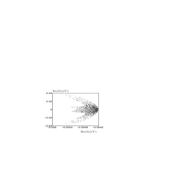
FIG. 1.: The parameter space of ($m_{0}$, $a$) and (${\rm Re}(b)$, ${\rm Im}(b)$) in Scenario (A), where only the normal neutrino mass hierarchy is allowed.

FIG. 2.: The parameter space of $\left({\rm Re}(m_{0}),{\rm Im}(m_{0})\right)$ and ($a$, $b$ or $c$) in Scenario (B) with the normal neutrino mass hierarchy.

FIG. 3.: The parameter space of $\left({\rm Re}(m_{0}),{\rm Im}(m_{0})\right)$ and ($a$, $b$ or $c$) in Scenario (B) with the inverted neutrino mass hierarchy.

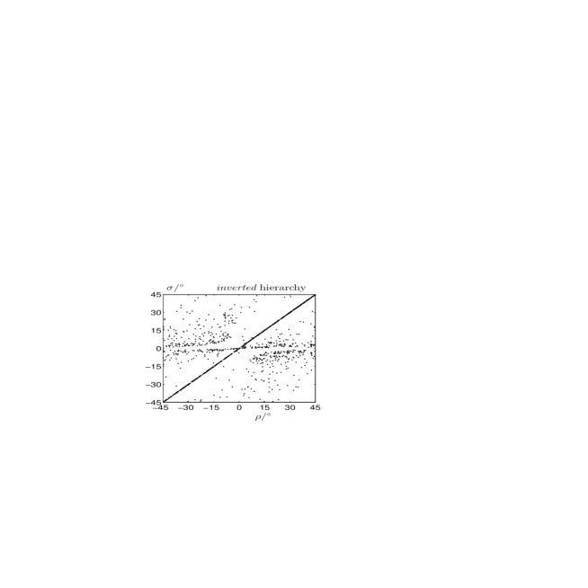
FIG. 4.: The parameter space of $\rho$ and $\sigma$ in Scenario (B) with the normal or inverted neutrino mass hierarchy. Note that the same parameter space can be obtained when $\rho\rightarrow\rho\pm n\pi/2$ and $\sigma\rightarrow\sigma\pm n\pi/2$ (for $n=1,2,3,\cdots$), as a straightforward consequence of Eq. (17).