Determining fundamental parameters of QCD on the lattice

Abstract

We summarize the status of determinations of fundamental parameters of QCD by the .

1 INTRODUCTION

The natural choice for the fundamental parameters of QCD are the renormalization group invariant (RGI) quark masses, $M_{i},i=\mathrm{u,d,...}$, and the $\Lambda$-parameter. The RGI masses do not depend on a renormalization scheme and the scheme dependence of the $\Lambda$-parameter is exactly given by a one-loop coefficient. These quantities are in principle free of perturbative uncertainties.

Their determination from low energy hadron data is a relevant mission for lattice QCD. Before entering details, we discuss a few aspects of more conventional determinations of $\alpha$ (and $\Lambda$). One considers experimental observables $O_{i}$ depending on an overall energy scale $q$ and possibly some additional kinematical variables denoted by $y$. The observables can be computed in a perturbative series which is usually written in terms of the $\overline{\mathrm{MS}}$ coupling $\alpha_{{\rm\overline{MS\kern-0.35002pt}\kern 0.35002pt}}=\bar{g}^{2}_{{\rm\overline{MS\kern-0.35002pt}\kern 0.35002pt}}/4\pi$, $(\mu=q)$

$$O_{i}(q,y)=\alpha_{{\rm\overline{MS\kern-0.35002pt}\kern 0.35002pt}}(\mu)+A_{i}(y)\alpha_{{\rm\overline{MS\kern-0.35002pt}\kern 0.35002pt}}^{2}(\mu)+\ldots\,\enspace.$$ (1)

For example $O_{i}$ may be constructed from jet cross sections and $y$ may be related to the details of the definition of a jet.

The renormalization group describes the energy dependence of $\bar{g}$ in a general scheme,

$$\mu{\partial\bar{g}\over\partial\mu} = \beta(\bar{g})\enspace,$$ (2)

here the $\beta$-function has an asymptotic expansion

$$\beta(\bar{g}) \buildrel{\bar{g}}\rightarrow 0\over{\sim} -{\bar{g}}^{3}\left\{b_{0}+{\bar{g}}^{2}b_{1}+\ldots\right\}\enspace,$$ (3)

$$b_{0}=\hbox{$1\over(4\pi)^{2}$}\bigl{(}11-\hbox{$2\over 3$}N_{\rm f}\bigr{)}\enspace,$$

$$b_{1}=\hbox{$1\over(4\pi)^{4}$}\bigl{(}102-\hbox{$38\over 3$}N_{\rm f}\bigr{)}\enspace,$$

with higher order coefficients $b_{i},\,i>1$ that depend on the scheme.

We note that – neglecting experimental uncertainties – $\alpha_{{\rm\overline{MS\kern-0.35002pt}\kern 0.35002pt}}$ extracted in this way is obtained with a precision given by the terms that are left out in eq. (1). In addition to (say) $\alpha^{3}$-terms, there are non-perturbative contributions which may originate from renormalons, instantons or, most importantly, may have an origin that no physicist has yet uncovered. Empirically, one observes that values of $\alpha_{{\rm\overline{MS\kern-0.35002pt}\kern 0.35002pt}}$ determined at different energies and evolved to a common reference point using eq. (2) including $b_{2}$ agree rather well with each other; the aforementioned uncertainties are apparently not very large. Nevertheless, the standard determinations of $\alpha$ are limited in precision because of these uncertainties and in particular if there was a significant discrepancy between $\alpha$ determined at different energies and/or processes it would be difficult to say whether this was due to the terms left out in eq. (1) or was due to terms missing in the Standard Model Lagrangian.

It is an obvious possibility, and at the same time a challenge, for lattice QCD to achieve a determination of $\alpha$ in one non-perturbatively (NP) well defined scheme at large $\mu$. There one may use the perturbative approximation for $\beta(\bar{g})$ inserted into the exact solution of eq. (2),

$$\Lambda = \mu\left(b_{0}\bar{g}^{2}(\mu)\right)^{-b1/(2b_{0}^{2})}{\rm e}^{-1/(2b_{0}\bar{g}^{2}(\mu))}$$

$$\times\exp\left\{-\int_{0}^{\bar{g}(\mu)}{\rm d}x\left[\hbox{$1\over\beta(x)$}+\hbox{$1\over b_{0}x^{3}$}-\hbox{$b_{1}\over b_{0}^{2}x$}\right]\right\}\enspace,$$

in order to extract the $\Lambda$-parameter.

1.1 Problem

In an implementation of this idea one needs to satisfy the following criteria.
$\bullet$ Compute $\alpha(\mu)$ at energy scales of $\mu\sim 10\,{\rm GeV}$ or higher in order to connect in a controlled manner to the perturbative regime.
$\bullet$ Keep $\mu$ removed from the lattice cutoff $a^{-1}$ to avoid large discretization effects and to be able to extrapolate to the continuum limit.
$\bullet$ Avoid finite size effects in the MC simulations by keeping the box size $L$ large compared to the inverse of the mass of the pion, $m_{\pi}$.

These conditions are summarized by

$$L\,\gg\,{1\over m_{\pi}}\,\sim\,{1\over 0.14{\rm GeV}}\,\,\gg\,\,{1\over\mu}\,\sim\,{1\over 10{\rm GeV}}\,\,\gg a\enspace,$$

which means that one must perform a MC-computation on an $N^{4}$ lattice with $N\equiv L/a\gg 70$: an impossible task for some time to come.

1.2 Solution

The simple solution is to identify the renormalization scale and the box size $L$ [1], and step up the energy scale recursively. Each step then requires only $L/a\gg 1$, see Fig. 1.

$${\rm HS}\quad\longrightarrow\quad {\rm SF}(\mu=1/{L_{\rm max}})$$

$${L_{\rm max}}={\rm O}(\hbox{$1\over 2$}{\rm fm})\qquad$$

$$\downarrow$$

$${\rm SF}(\mu=2/{L_{\rm max}})$$

$$\downarrow$$

$$\bullet$$

$$\bullet$$

$$\bullet$$

$$\downarrow$$

$${\rm SF}(\mu=2^{n}/{L_{\rm max}})$$

$$\quad\mbox{ \small PT}\quad\downarrow\quad\mbox{\small eq.~{}(\ref{e:lambda})}$$

DIS, jet-physics,

$$R_{\mathrm{had}}\mbox{ at }s=M_{Z}^{2}\quad\stackrel{{\scriptstyle\rm PT}}{{\longleftarrow}} \Lambda_{\rm QCD},M$$

Figure 1: The strategy for a non-perturbative computation of short distance parameters.

2 RUNNING OF THE COUPLING

We choose a NP defined Schrödinger functional renormalization scheme (SF) and set all renormalization conditions at zero quark mass (see [2] and references therein). An essential property of this scheme is the use of Dirichlet boundary conditions in time, which allow for MC simulations at vanishing quark mass.

2.1 The step scaling function

One vertical step in the figure is achieved as follows: we start from a given value of the coupling, $u=\bar{g}^{2}(L)$. When we change the length scale by a factor $2$, the coupling has a value $\bar{g}^{2}(2L)=u^{\prime}$ . The step scaling function, $\sigma$, is then defined as

$$\sigma(u) = u^{\prime}\enspace.$$ (5)

It is a discrete $\beta$-function whose knowledge allows for the recursive construction of the running coupling at discrete values of the length scale, $u_{k}=\bar{g}^{2}(2^{-k}L_{\rm max})\enspace,$ once a starting value $u_{\mathrm{max}}=\bar{g}^{2}(L_{\rm max})$ is specified. The step scaling function has a perturbative expansion $\sigma(u)=u+2b_{0}\ln(2)u^{2}+\ldots\enspace.$

On a lattice with finite spacing, $a$, it has an additional dependence on the resolution $a/L$. Its computation then consists of the following steps:
1. Choose an $(L/a)^{4}$ lattice ($1\leq x_{\mu}/a=\leq L/a$).
2. Tune the bare coupling $g_{0}$ such that the renormalized coupling $\bar{g}^{2}(L)$ has the value $u$ and tune the bare quark mass $m_{0}$ such that the PCAC-mass vanishes.
3. At the same values of $g_{0},m_{0}$, simulate a $(2L/a)^{4}$ lattice; compute $u^{\prime}=\bar{g}^{2}(2L)$. The lattice step scaling function is $\Sigma(u,a/L)=u^{\prime}$.
4. Repeat steps 1.–3. with different resolutions $L/a$ and extrapolate $\sigma(u)=\lim_{a/L\to 0}\Sigma(u,a/L)$.
Note that step 2. takes care of the renormalization and 3. determines the evolution of the renormalized coupling. The continuum extrapolation 4. is an essential part. In QCD, starting with the pure gauge theory, a lot of effort – both perturbative, analytical and by MC – has been invested in understanding this step properly. We do not have the space here to explain it in detail, but as a result of [4, 5, 3, 2, 6] and other work cited in these references, we are convinced that no systematic lattice errors are left.

3 RESULTS

We proceed directly to discussing the results. Numerical data for the step scaling function have been obtained for 7 values of $u$ in the range of $u=1.0$ to $u=3.3$ for QCD with $N_{\rm f}=2$ dynamical flavours [3, 2], while for $N_{\rm f}=0$ there are 11 points in $u$ between $u=0.9$ and $u=2.4$ [7, 5]. After taking the continuum limit, the extracted $\sigma(u)$ have a precision of around 0.5% at the smallest coupling (where it runs slowly) to 2% at the largest one. The numerical values of $\sigma(u)$ are then represented by a smooth interpolating function (a polynomial in $u$). With this function the running coupling can be constructed recursively; the result is shown in Fig. 3 and Fig. 4.

With a start value for the $\beta$-function taken from perturbation theory (3-loop) at the weakest coupling ($\alpha\approx 0.08$), one can also set up a recursion for the $\beta$-function itself [2].

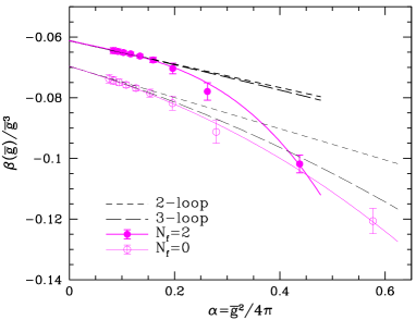
Figure 2: The QCD $\beta$–function in the SF scheme.

As Fig. 2 shows, its agreement with perturbation theory is excellent at weak couplings $\alpha<0.2$, while at the largest couplings significant deviations from perturbation theory are present for $N_{\rm f}=2$. Indeed the difference between non-perturbative points and 3-loop can’t be described by an effective 4-loop term with a reasonable coefficient. At the same time the perturbative series just by itself does not show signs of its failure at, say, $\alpha\approx 0.4$. Similar deviations from perturbation theory, at even somewhat smaller values of $\alpha$ have been found in the NP scale dependence of composite operators [8, 9].

Table 1: Lambda parameter in units of $r_{0}$ for $N_{\rm f}=2$.

	$u_{\rm max}=4.61$
$r_{0}/a$	$L_{\rm max}/a$	$\Lambda_{\overline{\mathrm{MS}}}\,r_{0}$
5.45(5)(20)	6.00(8)	0.610(25)
6.01(4)(22)	6.57(6)	0.614(24)
7.01(5)(15)	7.73(10)	0.609(16)

We return to the running couplings shown in Fig. 3 and Fig. 4. In the zero flavour case, also the region of $\mu$ of around $250\,{\rm MeV}$ was investigated with a specifically adapted strategy [10]. In this region, the SF coupling shows the rapid growth expected from a strong coupling expansion.

Initially, the graphs Fig. 3 and Fig. 4 are obtained for $\mu$ in units of $\mu_{\mathrm{min}}=1/L_{\rm max}$ defined by $\bar{g}^{2}(L_{\rm max})=u_{\mathrm{max}}$. One chooses $u_{\mathrm{max}}$ relatively large, but within the range covered by the non-perturbative computation of $\sigma(u)$. Since it has been verified that perturbative running sets in (in the SF scheme) at the larger $\mu$ that were simulated, one can use eq. (1) with the perturbative $\beta$-function in that region. In this way $L_{\rm max}$ can be expressed in units of $\Lambda^{-1}$:

$$N_{\rm f}=0 u_{\mathrm{max}}=3.48$$ (6)

$$\ln(\Lambda_{{\rm\overline{MS\kern-0.35002pt}\kern 0.35002pt}}L_{\rm max})=-0.84(8)$$

$$N_{\rm f}=2 u_{\mathrm{max}}=4.61$$ (7)

$$\ln(\Lambda_{{\rm\overline{MS\kern-0.35002pt}\kern 0.35002pt}}L_{\rm max})=-0.40(7)\,.$$

It remains to relate the artificially defined length scale $L_{\rm max}$ to an experimentally measurable low energy scale of QCD such as the proton mass or the kaon decay constant, $F_{\rm K}$. So far we have evaluated $L_{\rm max}$ in units of the scale parameter $r_{0}$, which has a precise definition in terms of the QCD static quark potential [11] and is well calculable on the lattice. But it is related to experiments only through potential models: $r_{0}\approx 0.5\,{\rm fm}$. For $N_{\rm f}=0$ the continuum limit is $L_{\rm max}/r_{0}=0.738(16)$, $\Lambda_{\overline{\mathrm{MS}}}^{(0)}r_{0}=0.60(5)$ [12].

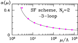
Figure 3: Running coupling for $N_{\rm f}=2$.

In the $N_{\rm f}=2$ theory, the situation is illustrated in Table 1 which relies on results for $r_{0}/a$ from [13, 14]. On the one hand, all the numbers are consistent, indicating that lattice spacing effects are small, on the other hand the first colum shows that $a$ is not yet varied very much. At the moment we quote $\Lambda_{\overline{\mathrm{MS}}}^{(2)}r_{0}=0.62(4)(4)$, where the second error generously covers the range of Table 1 as well as numbers obtained with $u_{\mathrm{max}}=3.65$ [2] and the first one comes from eq. (7).

4 DISCUSSION

The scale dependence of the SF coupling is close to perturbative below $\alpha_{\mathrm{SF}}=0.2$ and becomes non-perturbative above $\alpha_{\mathrm{SF}}=0.25$. In fact a strong coupling expansion suggests that this coupling grows exponentially for large $L$ and in the $N_{\rm f}=0$ theory it was possible to verify this behavior for $L$ close to $1\,{\rm fm}$ [10] (Fig. 4).

In the following table, we compare our results for $\Lambda_{\overline{\mathrm{MS}}}r_{0}$ to selected phenomenological ones, where we set $r_{0}=0.5\,{\rm fm}$.
$N_{\rm f}$: 0 2 4 5 [2, 7] 0.60(5) 0.62(6) [15] 0.74(10) 0.54(8) [16] 0.57(8)

There appears to be an irregular $N_{\rm f}$-dependence, but we note that
1.  the errors are not very small,
2.  the 4-flavour $\Lambda$ is related to the 5-flavour one by perturbation theory [17] which is then required to be accurate for $\mu\ll m_{\mathrm{beauty}}$.

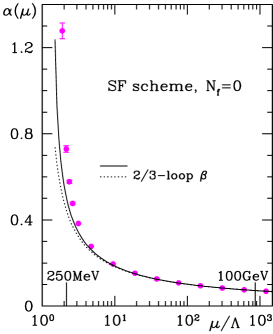
Figure 4: Running coupling for $N_{\rm f}=0$.

4.1 Improvements of lattice results

The replacement of $L_{\rm max}/r_{0}$ by $F_{\rm K}\times L_{\rm max}$ (computed at small enough light quark masses and small $a$) is the most urgent step and an effort is presently being made. Also the strange quark sea has to be included (“2+1”) and one should estimate the effects of the charm quark. Such 2+1 simulations are for example being carried out by JLQCD and CP-PACS, who have also studied the computation of the SF coupling with the gauge action they are using[18].

I am convinced that lattice results will yield the best controlled and most precise $\Lambda$ in the long run. The reason is simple: I essentially described all the sources of systematic errors and the kind of assumptions one has to make are minimal.

There is a large number of other results from lattice gauge theory, where $\alpha(\mu)$ is extracted from a quantity related to the cutoff: $\mu\sim a^{-1}$. Some of them cite a very small error [19]. As discussed for example in [20], it is, however, not easy to estimate the systematic errors in these computations, mainly because one cannot separate higher order perturbative corrections from discretization errors. It thus remains very desirable to carry out the program of Fig. 1 with good precision and the relevant number of flavors.

5 QUARK MASSES

The strategy discussed above is easily generalized to include the quark masses [5]. A useful ingredient is again to choose a mass independent renormalization scheme (even for ${m_{{\rm b}}}$) where ($i=$ up, down, strange …)

$$\kern 1.0pt\overline{\kern-1.0ptm\kern-1.0pt}\kern 1.0pt_{i}(\mu)=Z_{m}(\mu a,g_{0})\,m^{\mathrm{bare}}_{i}(g_{0})$$ (8)

with a flavour independent renormalization factor $Z_{m}(\mu a,g_{0})$. The scale dependence of the running masses can then be computed once and for all. The RGI masses are defined by

$$M_{i}=\lim_{\mu\to\infty}(2b_{0}\bar{g}^{2}(\mu))^{-d_{0}/2b_{0}}\,\kern 1.0pt\overline{\kern-1.0ptm\kern-1.0pt}\kern 1.0pt(\mu)_{i}$$ (9)

and we have

$$M_{i}/M_{j}=\kern 1.0pt\overline{\kern-1.0ptm\kern-1.0pt}\kern 1.0pt(\mu)_{i}/\kern 1.0pt\overline{\kern-1.0ptm\kern-1.0pt}\kern 1.0pt(\mu)_{j}=m^{\mathrm{bare}}_{i}/m^{\mathrm{bare}}_{j}\,.$$ (10)

In [5, 21] the renormalization problem has been solved non-perturbatively in the $N_{\rm f}=0,2$ theories: the $\mu$–dependence in the SF scheme was computed at the % level. Based on this the results in Table 2 were obtained. They may easily be converted to $\kern 1.0pt\overline{\kern-1.0ptm\kern-1.0pt}\kern 1.0pt_{{\rm\overline{MS\kern-0.35002pt}\kern 0.35002pt}}(\mu)$ if the desired renormalization scale $\mu$ is not too small.

Table 2: Quark masses determined with full NP renormalization and continuum limit. We use $r_{0}=0.5\,{\rm fm}$.

$i$	$N_{\rm f}$	input	$M_{i}/{\rm GeV}$	ref.
strange	0	$m_{\rm K},r_{0}$	0.137(05)	[22]
strange	2	$m_{\rm K},r_{0}$	0.137(27)	[21]
charm	0	$m_{\rm D},r_{0}$	1.654(45)	[23]
beauty	0	$m_{\rm B_{\rm s}},m_{\rm B_{\rm s}^{*}},r_{0}$	6.771(99)	[24]

For the charm and the beauty quark masses determinations with $N_{\rm f}>0$ and NP renormalization are still missing. However, in our opinion it is even quite early concerning the determinations of the light quark masses. Although some $N_{\rm f}$-dependence of the strange quark mass has been reported in the literature, one can presently not exclude that this is due to perturbative uncertainties or discretization errors.

Note that the quark masses computed in the quenched approximation were in a similar stage in 1996 but very soon afterwards the uncertainties shrunk by an order of magnitude due to NP renormalization and continuum extrapolations!

References

- [1] M. Lüscher, P. Weisz and U. Wolff, Nucl. Phys. B359 (1991) 221.
- [2] ALPHA, M. Della Morte et al., Nucl. Phys. B713 (2005) 378, hep-lat/0411025.
- [3] ALPHA, A. Bode et al., Phys. Lett. B515 (2001) 49, hep-lat/0105003.
- [4] ALPHA, A. Bode, P. Weisz and U. Wolff, Nucl. Phys. B576 (2000) 517, Erratum-ibid.B600:453,2001, Erratum-ibid.B608:481,2001, hep-lat/9911018.
- [5] ALPHA, S. Capitani et al., Nucl. Phys. B544 (1999) 669, hep-lat/9810063.
- [6] ALPHA, G. de Divitiis et al., Nucl. Phys. B437 (1995) 447, hep-lat/9411017.
- [7] M. Lüscher et al., Nucl. Phys. B413 (1994) 481, hep-lat/9309005.
- [8] ALPHA, M. Guagnelli et al., JHEP 03 (2006) 088, hep-lat/0505002.
- [9] ALPHA, J. Heitger, M. Kurth and R. Sommer, Nucl. Phys. B669 (2003) 173, hep-lat/0302019.
- [10] ALPHA, J. Heitger et al., Nucl. Phys. Proc. Suppl. 106 (2002) 859, hep-lat/0110201.
- [11] R. Sommer, Nucl. Phys. B411 (1994) 839, hep-lat/9310022.
- [12] S. Necco and R. Sommer, Nucl. Phys. B622 (2002) 328, hep-lat/0108008.
- [13] JLQCD, S. Aoki et al., Phys. Rev. D68 (2003) 054502, hep-lat/0212039.
- [14] QCDSF, M. Göckeler et al., (2004), hep-ph/0409312.
- [15] S. Bethke, (2004), hep-ex/0407021.
- [16] J. Blümlein, H. Böttcher and A. Guffanti, Nucl. Phys. Proc. Suppl. 135 (2004) 152, hep-ph/0407089.
- [17] W. Bernreuther and W. Wetzel, Nucl. Phys. B197 (1982) 228.
- [18] S. Takeda et al., Phys. Rev. D70 (2004) 074510, hep-lat/0408010.
- [19] HPQCD, Q. Mason et al., Phys. Rev. Lett. 95 (2005) 052002, hep-lat/0503005.
- [20] R. Sommer, (1997), hep-ph/9711243.
- [21] ALPHA, M. Della Morte et al., Nucl. Phys. B729 (2005) 117, hep-lat/0507035.
- [22] ALPHA, J. Garden et al., Nucl. Phys. B571 (2000) 237, hep-lat/9906013.
- [23] ALPHA, J. Rolf and S. Sint, JHEP 12 (2002) 007, hep-ph/0209255.
- [24] M. Della Morte et al., PoS LAT2005 (2005) 224, hep-lat/0509173.