Measurement of Renyi Entropies in Multiparticle Production: a Do-List II

Abstract

Recently suggested method of measuring Renyi entropies of multiparticle systems produced in high-energy collisions is presented in the form of a “do-list”, explaining explicitely how to perform the measurement and suggesting improvements in the treatment of the data.

PACS25.75.Gz, 13.65.+i

1 Introduction

A possibility to estimate the Renyi entropies [1] of the multiparticle systems created in high-energy collisions was suggested some time ago by two of us [2]. The method is based on observation of the event-by-event fluctuations or, more precisely, on measurement of coincidences between different events observed in collisions. Being classical in nature, the analysis of [2] could not, however, provide the absolute scale for entropy and thus the obtained numbers suffered from a serious uncertainty. Recently, we published several papers discussing a quantum approach to the same problem [3–5]. This allows to reduce the uncertainties of the classical treatment and to formulate the improvements of the method, leading to a more precise determination of Renyi entropies from data. Since the Renyi entropy gives the lower limit on the Shannon entropy [6], such measurements may provide essential information on the structure of the system produced in high-energy collisions [8].

In the present paper we collect the results of [3–5] in the form of a “do list”, i.e. of an explicit prescription how to perform the measurements and how to estimate the necessary corrections. We spell out explicitly the steps to be taken to implement effectively the results of [3–5]. The importance of the dependence of measurements on discretization of particle momenta and the role of (multi)particle correlations are emphasized. The paper may be considered as an extension of the previous publication with a similar title [9], but it can be read independently.

2 Selection of the phase-space region

As the first step in the process of measurement one has to select a phase-space region in which measurements are to be performed. This of course depends on the detector acceptance as well as on the physics one wants to investigate. The region cannot be too large because for large systems the method is difficult to apply (the requirements on statistics become too demanding). With a statistics of $10^{6}$ events, the region containing (on the average) $\approx 100$ or less particles should be possible to investigate. A reasonable procedure seems to be to start from a small region and then increase it until the errors become unacceptable.

Comment: The proposed measurement is not restricted to systems with large number of particles. It can be applied to any multiparticle system, e.g., to $e^{+}e^{-}$ annihilation, hadron–hadron collisions or peripheral nucleus-nucleus collisions. It was tested for the PYTHIA MC code for $pp$ collisions [10] and recently employed for data on hadron–hadron collisions by the NA22 collaboration [11].

3 Discretization of the spectrum

The selected region in momentum space should now be divided into bins. The size of the bins is — in principle — arbitrary. It turns out to be convenient to express it in the form

$$\Delta K_{x}\Delta K_{y}\Delta K_{z}=\left[\frac{2\pi}{l^{1/(l-1)}}\right]^{3/2}\frac{\kappa_{x}}{L_{x}}\frac{\kappa_{y}}{L_{y}}\frac{\kappa_{z}}{L_{z}}\,,$$ (1)

where $l$ is the rank of Renyi entropy to be measured, $\kappa_{x},\kappa_{y},\kappa_{z}$ are arbitrary (positive) parameters, and $L_{x}^{2},L_{y}^{2},L_{z}^{2}$ are the mean square radii of the system in configuration space, e.g.

$$L_{x}^{2}=\int(X-\bar{X})^{2}D(X,Y,Z)dXdYdZ\,.$$ (2)

Here $D(X,Y,Z)$ is the normalized distribution of positions of particle emission points in configuration space.

As seen from (1) the parameter $\kappa\equiv\kappa_{x}\kappa_{y}\kappa_{z}$, is a regulator of the size of the bins used for discretization of the spectrum. Note that $\kappa$ need not be constant through the selected momentum space. Actually it may be — generally — convenient to vary $\kappa$ with the position of the bin in momentum space. For example, in case of boost invariant distribution it is reasonable to discretize with bins of equal size in rapidity. The well-known equality $dK_{z}=E(K)dy$ suggests to take

$$\kappa_{z}=E(K_{z},K_{\perp})\kappa_{z}^{(0)}\,,$$ (3)

where $E(K_{z},K_{\perp})$ is the particle energy in the considered bin ($K_{z}$ and $K_{\perp}$ are the central values in this bin), while $\kappa_{z}^{(0)}$ is a constant.

Although the value of the measured Renyi entropy does not depend on the choice of $\kappa$, it should be emphasized that its selection does influence the accuracy of the measurement.

The number of bins cannot be too large if one wants to keep the statistical errors under control. It follows that (1) restricts the acceptable values of $\kappa$ and of the size of the momentum phase-space region which one may reasonably investigate at a given statistics of the experiment.

4 Description of an event

Using this procedure, an event is characterized by the number of particles in each bin, i.e. by a set of integer numbers $s\equiv m_{j}^{(i)}$, where $j=1,...J$ ($J$ is the total number of bins) and the superscript $(i)$ runs over all the kinds of particles present in the final state. These sets represent different states of the multiparticle system which were realized in the given experiment. The number of possible different sets is, generally, very large (for 5 bins and 100 indistinguishable particles one obtains about $5\times 10^{6}$ sets). This is, in fact, the main difficulty in the application of the method. It reflects the fact that the system we are dealing with has very many possible states.

Comment: It should be realized that, in practice, such a description is never complete, i.e., it never describes fully the event (even if the bin width is ignored). Most often some of the variables are summed over. This is the case, e.g., when one measures only charged particles. Then all the variables (i.e. multiplicities and momenta) related to neutral particles are summed over. It may be thus interesting to study reduced events, when even some of the measured variables (e.g. particle identity) are summed over (i.e. ignored).

5 Measurement of experimental coincidence probabilities

As explained in [2], the measurement of experimental coincidence probabilities is the basis of the method and therefore the most important step in the whole procedure.

The measurement consists of the simple counting how many times ($n_{s}$) any given set $s$ appears in the whole sample of events. Once the numbers $n_{s}$ are known for all sets, one forms the sums:

$$N{(l)}=\sum_{s}n_{s}(n_{s}-1)...(n_{s}-l+1)$$ (4)

with $l=1,2,3,...$ . Each sum formally runs over all the sets $s$ recorded in a given experiment, but nonvanishing contributions are given only by those which were recorded at least $l$ times. Thus $N(l)$ is the total number of observed coincidences of $l$ configurations and it can be recognized as the factorial moments [14] of the distribution of $n_{s}$ (in particular, $N(1)=N$, where $N$ is the total number of the events in the sample). The coincidence probability of $l$ configurations is thus given by

$$C^{\rm exp}(l)=\frac{N(l)}{N(N-1)...(N-l+1)}\approx\frac{N(l)}{N^{l}}\,.$$ (5)

Of course $C^{\rm exp}(1)=1$. As explained in [2], this ratio is equal to the$(l-1)$-th moment of the probability distribution: $C^{\rm exp}(l)=\sum_{s}(p_{s})^{l}$.

It is clear that two identical configurations must have the same total number of particles measured in the phase-space region considered, say $M$. It turns out that to obtain Renyi entropies, it is necessary to determine $C^{\rm exp}(l)$ for each multiplicity separately. We shall denote these numbers by $C_{M}^{\rm exp}(l)$.

The error of $C^{\rm exp}(l)$ is determined by the error of the numerator in (5). One finds approximately $[\Delta N(l)]^{2}\approx l!N(l)$.

6 Renyi entropies

To obtain the Renyi entropies:

$$H(l)=\frac{1}{1-l}\log C(l)$$ (6)

it is necessary to determine the true coincidence probabilities:

$$C(l)={\rm Tr}[\rho]^{l}$$ (7)

with $\rho$ being the density matrix of the system. $C(l)$ can be expressed in terms of the true coincidence probabilities $C_{M}(l)$ at fixed multiplicity:

$$C(l)=\sum_{M}[P(M)]^{l}C_{M}(l)\,,$$ (8)

where $P(M)$ is the multiplicity distribution.

The relation between $C_{M}(l)$ and the measured $C_{M}^{\rm exp}(l)$ was studied in [3–5]. It can be summarized as follows:

$$C_{M}(l)=C_{M}^{\rm exp}(l){\mit\Lambda}_{M}(l){\mit\Psi}_{M}(l)\,.$$ (9)

The correction factors ${\mit\Lambda}_{M}$ and ${\mit\Psi}_{M}$ depend on $M$ (this is the reason why $C_{M}^{\rm exp}(l)$ must be determined for every multiplicity separately). They are discussed in the next two sections.

7 Estimate of ${\mit\Lambda}_{M}(l)$

Denoting the (3M dimensional) normalized momentum distribution by

$$w(K)\equiv e^{-v(K)},$$ (10)

and the size of a bin $j$ by $\omega_{j}$ the correction factor ${\mit\Lambda}_{M}(l)$ is given by

$${\mit\Lambda}_{M}(l)=\frac{\sum_{j}\kappa_{j}^{M}\left\langle[w(K)]^{l}\right\rangle_{\omega_{j}}}{\sum_{j}\kappa_{j}^{Ml}[\bar{w}_{\omega_{j}}]^{l}}\,,$$ (11)

where the summation extends over all (3M-dimensional) bins and $\langle...\rangle_{\omega_{j}}$ denotes the average over a bin of volume $(\omega_{j})^{M}$, e.g.,

$$\langle[w(K)]^{l}\rangle_{\omega_{j}}=\frac{1}{\omega_{j}}\int\limits_{\omega_{j}}d^{3M}K[w(K)]^{l}\,.$$ (12)

We have also introduced the shorthand

$$\bar{w}_{\omega}(K)\equiv\frac{1}{\omega}\int\limits_{\omega}d^{3M}Kw(K)=\langle w(K)\rangle_{\omega}.$$ (13)

To estimate ${\mit\Lambda}_{M}(l)$ we observe that summations in numerator and denominator of (11) can be expressed as integrals over the considered phase-space region. We thus have

$${\mit\Lambda}_{M}(l)=\frac{\int\limits d^{3M}K[\kappa(K)]^{M}[w(K)]^{l}}{\int\limits d^{3M}K[\kappa(K)]^{Ml}[\bar{w}_{\omega}(K)]^{l}}\,.$$ (14)

If $\kappa$ is independent of the bin (i.e. independent of $K$), this formula simplifies into

$${\mit\Lambda}_{M}(l)=\kappa^{-M(l-1)}\hat{{\mit\Lambda}}_{M}(l)\;,\qquad\hat{{\mit\Lambda}}_{M}(l)=\frac{\int\limits d^{3M}K[w(K)]^{l}}{\int\limits d^{3M}K[\bar{w}_{\omega}(K)]^{l}}\,.$$ (15)

One sees that in this case $\hat{{\mit\Lambda}}_{M}(l)$ tends to one if the size of the bins is small enough (i.e. when $w(K)$ can be treated as constant within one bin). Then the value of ${\mit\Lambda}_{M}(l)$ is under full control.

If the bins are not small enough, one sees from (14) and (15) that ${\mit\Lambda}_{M}(l)$ can be estimated using the MC code appropriate for the given process. For the numerator this is rather straightforward. For the denominator, it is necessary to construct first the “smeared” MC which ignores the difference between the momenta of particles within each bin.

A simpler, but less precise, method is to ignore correlations between particles and write the distribution $w(K)$ in form of the product

$$w(K)=f(K_{1})...f(K_{M})\,,$$ (16)

where $f(K)$ is the single-particle momentum distribution.

In this case we obtain

$${\mit\Lambda}_{M}(l)=[\lambda(l)]^{M}$$ (17)

with

$$\lambda(l)=\frac{\int\limits d^{3}K\kappa(K)[f(K)]^{l}}{\int\limits d^{3}K[\kappa(K)\bar{f}_{\omega}(K)]^{l}}$$ (18)

and thus $\lambda(l)$ can be fairly easily evaluated numerically or even analytically.

8 Estimate of ${\mit\Psi}_{M}(l)$

The second correcting factor ${\mit\Psi}_{M}$ is given by the formula [4]

$${\mit\Psi}_{M}(l)=\frac{\int d^{3M}K[w(K)]^{l}{\mit\Theta}_{l}(K)}{\int d^{3M}K[w(K)]^{l}}\,,$$ (19)

where

$$[{\mit\Theta}_{l}(K)]^{-1}={\rm Det}\left[1+\sum_{s=1}a_{s}(l)[T]^{s}\right]$$ (20)

and

$$a_{s}(l)=\frac{1}{2^{s}}\frac{(l-1)!}{(2s+1)!(l-2s-1)!}\,.$$ (21)

$T$ is the symmetric $3M\times 3M$ matrix

$$T_{m\alpha,n\beta}=\frac{1}{L_{\alpha}}V_{m\alpha,n\beta}\frac{1}{L_{\beta}}$$ (22)

with

$$V_{m\alpha,n\beta}\equiv\frac{\partial}{\partial K_{m\alpha}}\frac{\partial}{\partial K_{n\beta}}v(K)\,.$$ (23)

Here $m,n=1,...,M$ label the particles and $\alpha,\beta=x,y,z$ denote the space directions.

It is seen from these formulae that ${\mit\Psi}_{M}(l)$ is independent of the bin size and thus cannot be influenced by selection of $\kappa$. It does depend, however, on the size of the system in configuration space ($L_{x},L_{y},L_{z}$). Moreover, as explained in [4], Eq. (19) represents an expansion in powers of $L^{-1}$ and thus can only be trusted if $L$ is large enough, so that ${\mit\Psi}_{M}(l)$ is not too different from one.

Note that (21) implies that the sum in (20) is finite, because all $a_{s}(l)$ vanish for $s\geq(l-1)/2$. In particular for $l=2$ we obtain ${\mit\Theta}_{2}=1$ and thus also ${\mit\Psi}_{M}(2)=1$. For the other two practically interesting cases ($l=3,4$), the sum reduces to just one term with

$$a_{1}(3)=\frac{1}{12}\,,\qquad a_{1}(4)=\frac{1}{4}\,.$$ (24)

Again, a MC code seems to be the best method to estimate ${\mit\Psi}_{M}(l)$. Indeed, Eq. (19) can be rewritten as

$${\mit\Psi}_{M}(l)=\int d^{M}KP_{l}(K){\mit\Theta}(K)=\langle{\mit\Theta}\rangle,$$ (25)

where the probability distribution $P_{l}(K)$ is defined as

$$P_{l}(K)=\frac{[w(K)]^{l}}{\int d^{3}K[w(K)]^{l}}\,.$$ (26)

To construct ${\mit\Theta}(K)$, however, an analytic formula for $w(K)$ is necessary, as seen from (22) and (23). This may be a difficulty.

If correlations between particles are neglected, the matrix $T_{m\alpha,n\beta}$ is diagonal in $(m,n)$ and the calculation of the determinant in (20) is greatly simplified. We write

$$v(K)=\sum_{m=1}^{M}u(K_{m})$$ (27)

and thus

$$V_{m\alpha,n\beta}=\delta_{mn}\partial_{m\alpha}\partial_{m\beta}u(K_{m}).$$ (28)

We shall only consider $l=3$ (${\mit\Psi}_{M}(2)=1$). We have

$$[{\mit\Theta}_{l}(K)]^{-1}={\rm Det}\left[1+\frac{1}{12}[T]^{s}\right]=\prod_{m=1}^{M}D(K_{m}),$$ (29)

where $D(K_{m})$ is the determinant of the $3\times 3$ matrix

$$D(K_{m})={\rm Det}\left[1+\frac{1}{12}\frac{\partial_{m\alpha}\partial_{m\beta}u(K_{m})}{L_{\alpha}L_{\beta}}\right].$$ (30)

Further simplifications are possible if the system is cylindrically symmetric, i.e., if $u(K)=u(k_{\perp},k_{\parallel})$. Then

$$D(K)=A\left[A^{2}+A(k_{\perp}^{2}B+\zeta)+k_{\perp}^{2}(B\zeta-C^{2})\right]\,,$$ (31)

where

$$A = 1+\frac{1}{12L_{\perp}^{2}}\frac{1}{k_{\perp}}\frac{\partial u}{\partial k_{\perp}}\,,\quad\;\;B=\frac{1}{12L_{\perp}^{2}k_{\perp}^{2}}\left[\frac{\partial^{2}u}{\partial k_{\perp}^{2}}-\frac{1}{k_{\perp}}\frac{\partial u}{\partial k_{\perp}}\right]\,,$$

$$C = \frac{1}{12L_{\perp}L_{\parallel}k_{\perp}}\frac{\partial^{2}u}{\partial k_{\parallel}\partial k_{\perp}}\,,\quad\zeta=\frac{1}{12L_{\parallel}^{2}}\frac{\partial^{2}u}{\partial k_{\parallel}^{2}}-\frac{1}{12L_{\perp}^{2}}\frac{1}{k_{\perp}}\frac{\partial u}{\partial k_{\perp}}$$ (32)

and the correction is given by

$${\mit\Psi}_{M}(3)=\left[\frac{\int\left[e^{-3u(K)}/D(K)\right]dk_{\perp}^{2}dk_{\parallel}}{\int e^{-3u(K)}dk_{\perp}^{2}dk_{\parallel}}\right]^{M}\,.$$ (33)

9 Remarks on size of the region in momentum space

The main difficulty in the measurements is to find a sufficient number of coincidences (to keep the statistical error under control). Therefore it is necessary to limit the size of the region in momentum space where the measurement is performed. This reduces the number of particles and thus increases the probability of coincidence. Below we estimate the practical consequences of this requirement.

9.1 Consequences of boost-invariance

Consider first the longitudinal momentum. If the system is approximately boost-invariant, one expects an approximate linear relation between the considered interval in longitudinal momentum ($\delta K_{z}$) and the size of the corresponding region in the configuration space ($L_{z}$, defined as the region from which the emitted particles end up in $\delta K_{z}$):

$$L_{z}\approx\frac{\delta K_{z}}{h^{2}}\,,$$ (34)

where the proportionality coefficient can be approximated by [15]

$$h^{2}=\frac{m_{\perp}}{\tau_{0}}$$ (35)

while $m_{\perp}$ is the transverse mass of the produced particle and $\tau_{0}$ is its proper time at freeze-out.

The conclusion is that the size of the selected region in longitudinal momentum determines the size of the corresponding region in configuration space. Consequently, the size of the selected region in longitudinal momentum cannot be too small (if we want the size $L_{z}$ in z-direction to be large enough for the analysis of this paper to be valid). Note that these remarks do not refer to the choice of the binning (discretization) but to the size of the momentum region in which the measurement is performed.

9.2 Uncorrelated distribution in azimuthal angle

Great improvement in the feasibility of measurement can be obtained if correlations between particles are weak and can be neglected. This is particularly effective if there are no correlations between various segments of the distribution in azimuthal angle. In this case the probability to observe a coincidence in the full azimuthal angle ($2\pi$) equals the square of the probability to observe a coincidence in half of the full angle ($\pi$). Therefore it is enough to observe the coincidences separately in two regions of size $\pi$ where the coincidence probability is much larger. Consequently, one needs much fewer events to obtain a decent statistics of coincidences (and thus a decent error of the measurement). The effect can be made even stronger if independence is observed for smaller regions of azimuthal angle. The procedure requires, of course, a careful checking with the data.

10 Numerical estimates

To obtain an idea about the size of corrections ${\mit\Lambda}_{M}(l)$ and ${\mit\Psi}_{M}(l)$ we shall now explicitely evaluate them in a simplified model where particles are uncorrelated and the single particle momentum distribution is axially symmetric and boost-invariant. The transverse momentum distribution is taken in the Boltzmann form. Thus we have

$$w(k_{\perp},k_{z})d^{2}k_{\perp}dk_{z} = Ae^{-\sqrt{k_{\perp}^{2}+m^{2}}/T}d^{2}k_{\perp}dy$$ (36)

$$= \frac{Ae^{-\sqrt{k_{\perp}^{2}+m^{2}}/T}}{\sqrt{k_{\perp}^{2}+k_{z}^{2}+m^{2}}}d^{2}k_{\perp}dk_{z}\,,$$

where $A$ is a normalization constant chosen such that $\int\!\!w(k_{\perp},k_{z})d^{2}k_{\perp}dk_{z}\!=\!1$. Consider first ${\mit\Lambda}_{M}(l)=[\lambda(l)]^{M}$ with

$$\lambda(l)=\frac{\frac{1}{\omega_{\perp}\delta k_{z}}\sum_{\rm bins}\int\limits_{\omega_{\perp}}d^{2}k_{\perp}e^{-lm_{\perp}/T}\int\limits_{\delta k_{z}}\frac{dk_{z}}{[k_{z}^{2}+m_{\perp}^{2}]^{l/2}}}{\frac{1}{[\omega_{\perp}\delta k_{z}]^{l}}\sum_{\rm bins}\left[\int\limits_{\omega_{\perp}}d^{2}k_{\perp}e^{-m_{\perp}/T}\int\limits_{\delta k_{z}}\frac{dk_{z}}{\sqrt{k_{z}^{2}+m_{\perp}^{2}}}\right]^{l}}\,,$$ (37)

where

$$\delta k_{z}=\frac{\sqrt{2\pi}}{[\sqrt{l}]^{1/(l-1)}L_{z}}\;,\qquad\omega_{\perp}\equiv\pi\delta k_{\perp}^{2}=\frac{2\pi}{l^{1/(l-1)}L_{\perp}^{2}}\,.$$ (38)

In figure 1 the correction factor

$$\delta_{2}=\frac{H(2)^{\rm exp}-H(2)}{H(2)^{\rm exp}}$$ (39)

is plotted as function of $L_{\perp}/\kappa_{\perp}$ (with $\kappa_{\perp}$ independent of $K$) for $L_{z}$ = 1 fm, $\kappa_{z}=1$ and two values of $T$. The longitudinal momentum interval was fixed by $-0.38$ GeV $\leq k_{z}\leq$ 0.38 GeV. One sees that for $L_{\perp}/\kappa_{\perp}$ greater than 1 fm the correction is small.

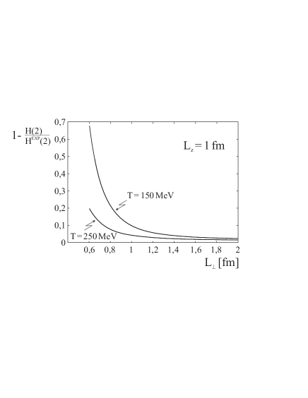
Figure 1: The correction factor $1-H(2)/H^{\rm exp}(2)$ plotted versus $L_{\perp}/\kappa_{\perp}$ with a constant $\kappa_{\perp}$ and $\kappa_{z}=1$. Other parameters are indicated in the figure. One sees that for $L_{\perp}/\kappa_{\perp}\geq$ 1 fm the correction is pretty small.

It should be emphasized that, as discussed already in Section 7, the correction factor to $H_{2}$ can be fully controlled with a good precision if the bins selected for discretization are small enough. If the size $L_{\perp}$ of the system is small, this can be achieved by a proper choice of the parameter $\kappa$. The results shown in figure 1 demonstrate that to this end it is enough to take $L_{\perp}/\kappa_{\perp}$ larger than 1 fm. Since the measurement of $H_{2}$ provides an effective lower limit on the value of the entropy of the system [7], it is reassuring that in this simple way the errors can be minimized and reliably estimated.

For $l\geq 3$ both ${\mit\Lambda}_{M}(l)=[\lambda(l)]^{M}$ and ${\mit\Psi}_{M}(l)\equiv[p(l)]^{M}$ are important. This creates a new problem. Indeed, since the correction factor ${\mit\Psi}_{M}(l)$ is insensitive to the bin size, it cannot be eliminated by a proper discretization (${\mit\Psi}_{M}(l)$ does not depend on $\kappa$ and thus cannot be adjusted at will).

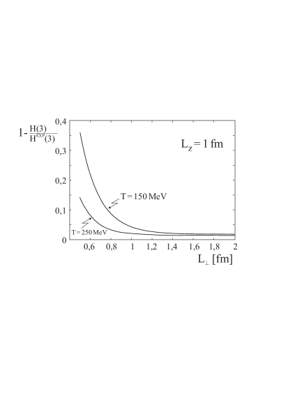
Figure 2: The correction factor $1-H(3)/H^{\rm exp}(3)$ plotted versus $L_{\perp}$ with $\kappa_{\perp}=\kappa_{z}=1$.

In figure 2 the correction factor

$$\delta_{3}\equiv\frac{H(3)^{\rm exp}-H(3)}{H(3)^{\rm exp}}$$ (40)

is plotted versus $L_{\perp}$ for $\kappa_{\perp}=\kappa_{z}=1$ and for the same parameters as in figure 1. It is seen that the corrections are reasonably small for $L_{\perp}>1$ fm but become dangerously large for smaller radii. Thus for $l\geq 3$ the method seems safe for heavy ion collisions but cannot be easily justified for systems with linear size smaller than 1 fm.

11 Shannon entropy

The Shannon entropy $S$ (i.e. the standard statistical entropy) is formally equal to the limit of $H(l)$ as $l\!\!\rightarrow\!\!1$ and thus can only be obtained by extrapolation from a series of measured values: $H(l)=H(2),H(3),...$ to $l=1\,$. Of course such an extrapolation procedure is not unique and introduces a serious uncertainty [16]. The main point is, as usual, to choose the “best” extrapolation formula, i.e. the functional dependence of $H(l)$ on $l$ which will be used to reach the point $l=1$ from the measured points $l=2,3,...$ . This form can only be guessed on the basis of physics arguments (or prejudices).

In [2] it was suggested to use

$$H(l)=a\frac{\log l}{l-1}+a_{0}+a_{1}(l-1)+a_{2}(l-1)^{2}+\dots\;,$$ (41)

where the number of terms is determined by the number of measured Renyi entropies. This formula turned out to be very effective in reproducing the correct value of entropy for some typical distributions encountered in high-energy collisions.

Another possibility is to use

$$H(l)=a_{0}+\frac{a_{1}}{l}+\frac{a_{2}}{l^{2}}+\dots$$ (42)

suggested by the formula for the free gas of massless bosons.

It will be interesting to compare the results from these two formulae.

Comment: The measured values of the Renyi entropies give valuable information about the system and thus are of great interest, independently of the accuracy of the extrapolation [17]. Moreover, from the inequality [6]

$$S\geq H(l)\geq H(l+1)\,,$$ (43)

valid for any $l>1$, we deduce that a measurement of any Renyi entropy gives an exact lower bound for $S$. It is well known that this is important information about the quark–gluon plasma [8].

12 Comparison of different regions: Additivity

Measurements of the entropies $H(l)$ and $S$, as described above, can be performed independently (and — in fact — simultaneously) in different momentum regions. The results should give information on the entropy density and its possible dependence on the region in momentum space (e.g., it seems likely that the results in the central rapidity region may be rather different from those in the projectile or target fragmentation region). Furthermore, it is important to verify to what extent the obtained entropies are additive, i.e., whether the entropies measured in a region $R$ which is the sum of two regions $R_{1}$ and $R_{2}$ satisfy

$$H(l)(R)=H(l)(R_{1})+H(l)(R_{2})\rightarrow S(R)=S(R_{1})+S(R_{2})\,.$$ (44)

Eq. (44) should be satisfied if there are no strong correlations between the particles belonging to the regions $R_{1}$ and $R_{2}$. Thus, verification of (44) gives information about the correlations between different phase-space regions.

Comment: It may be worth pointing out that the additivity (44) can be more precisely tested for Renyi entropies ($H(l)$) than for the Shannon entropy ($S$), where the extrapolation procedure (described in Section 6) always introduces an additional uncertainty. Since deviations from additivity signal correlations, this is an interesting problem in itself.

13 Conclusions

In conclusion, we have shown that the measurement of Renyi entropies in limited regions of phase-space is feasible and thus important information on the entropy of the system [8, 7] is possible to obtain. Moreover, even the simplest tests of the general scaling and additivity rules can provide essential information on fluctuations and on correlations in the system. It should be emphasized that for these tests the Renyi entropies turn out to be even more useful than the standard Shannon entropy.

We thank K. Fiałkowski and W. Kittel for discussions. This investigation was partly supported by the MEiN research grant 1 P03B 045 29 (2005–2008).

Appendix:
Various examples of probability distributions

Distributions with exponential tail

Consider the distribution

$$P(r_{i})=Ur_{i}^{\alpha}e^{-(r_{i}/a)^{\beta}}\delta r_{i}\,,$$ (45)

where $\delta r_{i}$ is small, so that we can replace everywhere the summations by integrals. We also assume that $\delta r_{i}={\rm const}=\delta$. With this assumption the normalization factor $U$ is given by

$$U^{-1}=\int r^{\alpha}e^{-(r/a)^{\beta}}dr=\frac{1}{\beta}a^{(\alpha+1)}{\mit\Gamma}\left[\frac{\alpha+1}{\beta}\right]\,.$$ (46)

The distribution (45) covers a wide range of different distributions. E.g., for $(\alpha=0,\,\beta=2)$ one obtains a Gaussian, for $\beta=1$ (and arbitrary $\alpha$), a Gamma distribution (including, as a special case the exponential distribution).

A fairly straightforward calculation gives

$$H(l)=\log\left[\frac{a}{\delta}\frac{{\mit\Gamma}[(\alpha\!+\!1)/\beta]}{\beta}\right]\!+\!\frac{1}{\beta}\frac{l\alpha\!+\!1}{l-1}\log l-\frac{1}{l\!-\!1}\log\left[\frac{{\mit\Gamma}[(l\alpha\!+\!1)/\beta]}{{\mit\Gamma}[(\alpha+1)/\beta]}\right]$$ (47)

and thus

$$S=\log\left[\frac{a{\mit\Gamma}[(\alpha+1)/\beta]}{\beta\delta}\right]+\frac{\alpha+1}{\beta}-\frac{\alpha}{\beta}\psi[(\alpha+1)/\beta]\,.$$ (48)

In particular, for a Gaussian we have

$$H_{G}(l)=\log\left[\frac{a\sqrt{\pi}}{\delta}\right]+\frac{\log l}{2(l-1)}\,.$$ (49)

Power law

$$P(r)dr\!=\!\lambda a^{\lambda}\frac{dr}{(a+r)^{1+\lambda}}\,,$$ (50)

$$C(l)\!=\!\lambda^{l}a^{l\lambda}\delta^{l-1}\!\!\int\limits_{0}^{\infty}\!\!\frac{dr}{(a\!+\!r)^{l(1+\lambda)}}\!=\!\frac{\lambda^{l}a^{l\lambda}\delta^{l-1}}{(l\lambda\!+\!l\!-\!1)a^{l\lambda+l-1}}\!=\!\left[\frac{\delta}{a}\right]^{l-1}\!\!\!\!\frac{\lambda^{l}}{l\lambda+l-1},$$ (51)

$$H(l) = \log(a/\delta)+\frac{1}{l-1}\log\left(1+(l-1)\frac{1+\lambda}{\lambda}\right)-\log\lambda\,,$$ (52)

$$S = \log(a/\delta)+\frac{1+\lambda}{\lambda}-\log\lambda\,.$$ (53)

Sum of Gaussians

Consider probability distribution which is a sum of two identical Gaussians separated by distance $2R$. This can be written as

$$P(r)=\frac{1}{a\sqrt{\pi}}\left[\lambda_{-}e^{-(r+R)^{2}/a^{2}}+\lambda_{+}e^{-(r-R)^{2}/a^{2}}\right],$$ (54)

where $\lambda_{+}+\lambda_{-}=1$, and gives

$$C(l) = \frac{\delta^{l-1}}{[a\sqrt{\pi}]^{l}}\sum_{j=0}^{l}\frac{l!}{j!(l-j)!}\lambda_{-}^{j}\lambda_{+}^{l-j}\int dre^{-j(r+R)^{2}/a^{2}}e^{-(l-j)(r-R)^{2}/a^{2}}$$ (55)

$$= \frac{\delta^{l-1}}{[a\sqrt{\pi}]^{l-1}\sqrt{l}}\sum_{j=0}^{l}\frac{l!}{j!(l-j)!}\lambda_{-}^{j}\lambda_{+}^{l-j}e^{-4R^{2}j(l-j)/(la^{2})}\,.$$

One sees that in the limit of $R/a$ very large, i.e. for well-separated Gaussians, only the terms with $j=0$ and $j=l$ contribute and we have

$$C(l)=C_{G}(l)\left(\lambda_{-}^{l}+\lambda_{+}^{l}\right)\,,$$ (56)

which simply adds a constant term to the entropy of a single Gaussian.

If $\lambda_{-}=\lambda_{+}=1/2$, we have $\lambda_{-}^{l}+\lambda_{+}^{l}=(1/2)^{l-1}$ and thus

$$H(l)=H_{G}(l)+\log 2\,.$$ (57)

It is not difficult to see that for $N$ well-separated Gaussians one obtains

$$H(l)=H_{G}(l)-\frac{1}{l-1}\log\left(\sum_{i=1}^{N}(\lambda_{i})^{l}\right)$$ (58)

If all Gaussians have equal weights $l=1/N$, one obtains

$$H(l)=H_{G}(l)+\log N$$ (59)

This result is valid for any set of well-separated distributions.

References

- [1] A. Renyi, Acta Math. Sci. Hung. 10, 193 (1959); see also: “On Measures of Information and Entropy”, in Proceedings 4-th Berkeley Symposium Math. Stat. Prob. Vol. 1 (1961) p.547.
- [2] A. Bialas, W. Czyz, Phys. Rev. D61, 074021 (2000).
- [3] A. Bialas, W. Czyz, K. Zalewski, Acta Phys. Pol. B 36, 3109 (2005); Phys. Lett. B633, 479 (2006).
- [4] A. Bialas, K. Zalewski, Acta Phys. Pol. B 37, 495 (2006).
- [5] A. Bialas, W. Czyz, K. Zalewski, Phys. Rev. C73, 034912 (2006).
- [6] See, e.g., C. Beck, F. Schloegl, Thermodynamics of Chaotic Systems, Cambridge U. Press, Cambridge 1993.
- [7] A. Bialas, W. Czyz, K. Zalewski, Eur. Phys. J., in print.
- [8] For a recent discussion see, e.g. B. Muller, K. Rajagopal, Eur. Phys. J. C43, 15 (2005) and references therein.
- [9] A. Bialas, W. Czyz, Acta Phys. Pol. B 31, 687 (2000).
- [10] K. Fialkowski, R. Wit, Phys. Rev. D62, 114016 (2000).
- [11] M. Atayan et al. [NA22 Collaboration], Acta Phys. Pol. B 36, 2969 (2005).
- [12] A. Bialas, W. Czyz, J. Wosiek, Acta Phys. Pol. B 30, 107 (1999).
- [13] S.K. Ma, Statistical Mechanics, World Scientific, Singapore 1985; S.K. Ma,J. Stat. Phys. 26, 221 (1981).
- [14] A. Bialas, R. Peschanski, Nucl. Phys. B273, 703 (1986).
- [15] K. Gottfried, Phys. Rev. Lett. 32, 957 (1974); J.D. Bjorken, Phys. Rev. D27, 140 (1983); A. Bialas, K. Zalewski, Acta Phys. Pol. B 30, 359 (1999).
- [16] See, e.g., K. Zyczkowski, Open Sys. and Information Dyn. 10, 297 (2003).
- [17] Some examples are discussed in A. Bialas, W. Czyz, Acta Phys. Pol. B 31, 2803 (2000); 34, 3363 (2003).