Phase-shift analysis of low-energy $\pi^{\pm}p$ elastic-scattering data

Abstract

Using electromagnetic corrections previously calculated by means of a potential model, we have made a phase-shift analysis of the $\pi^{\pm}p$ elastic-scattering data up to a pion laboratory kinetic energy of $100$ MeV. The hadronic interaction was assumed to be isospin invariant. We found that it was possible to obtain self-consistent databases by removing very few measurements. A pion-nucleon model, based on s- and u-channel diagrams with $N$ and $\Delta$ in the intermediate states, and $\sigma$ and $\rho$ t-channel exchanges, was fitted to the elastic-scattering database obtained after the removal of the outliers. The model-parameter values showed an impressive stability when the database was subjected to different criteria for the rejection of experiments. Our result for the pseudovector $\pi NN$ coupling constant (in the standard form) is $0.0733\pm 0.0014$. The six hadronic phase shifts up to $100$ MeV are given in tabulated form. We also give the values of the $s$-wave scattering lengths and the $p$-wave scattering volumes. Big differences in the $s$-wave part of the interaction were observed when comparing our hadronic phase shifts with those of the current GWU solution. We demonstrate that the hadronic phase shifts obtained from the analysis of the elastic-scattering data cannot reproduce the measurements of the $\pi^{-}p$ charge-exchange reaction, thus corroborating past evidence that the hadronic interaction violates isospin invariance. Assuming the validity of the result obtained within the framework of chiral perturbation theory, that the mass difference between the $u$- and the $d$-quark has only a very small effect on the isospin invariance of the purely hadronic interaction, the isospin-invariance violation revealed by the data must arise from the fact that we are dealing with a hadronic interaction which still contains residual effects of electromagnetic origin.
PACS: 13.75.Gx; 25.80.Dj; 25.80.Gn

, , , ,

^∗Corresponding author. E-mail address: evangelos.matsinos@varian.com. Tel.: +41 56 2030460. Fax: +41 56 2030405

1 Introduction

In two previous papers [1, 2], we presented the results of a new evaluation of the electromagnetic (EM) corrections which have to be applied in a phase-shift analysis (PSA) of the $\pi^{\pm}p$ elastic-scattering data at low energies (pion laboratory kinetic energy $T\leq 100$ MeV) in order to extract the hadronic phase shifts. The calculation used relativised Schrödinger equations containing the sum of an EM and a hadronic potential; the hadronic potential was assumed to be isospin invariant. We gave reasons for accepting the new corrections as more reliable than the ones obtained by the NORDITA group [3] in the late 1970s. For the $\pi^{+}p$ scattering data, the corrections $C_{0+}^{+}$, $C_{1-}^{+}$ and $C_{1+}^{+}$ for the $s$, $p_{1/2}$ and $p_{3/2}$ waves are given in Table 1 of Ref. [1]. For the $\pi^{-}p$ scattering data, the corrections $C^{1/2}$, $C^{3/2}$ and $\Delta{\phi}$ are listed in Tables 1-3 of Ref. [2].

In this paper, we present the results of a PSA of the $\pi^{\pm}p$ elastic-scattering data for $T\leq 100$ MeV which was performed using these new EM corrections. We have imposed two important restrictions on the experimental data.

First, in contrast to the Karlsruhe analyses [4] and to the modern GWU (formerly, VPI) solutions [5], we have chosen to analyse the elastic-scattering data separately. There is an important reason for this decision. As pointed out in Refs. [1, 2], what we called hadronic potentials (in those papers) are not the purely hadronic potentials which model the hadronic dynamics in the absence of the EM interaction; they contain residual EM effects, and we henceforth call them ‘electromagnetically modified’ (em-modified, for short) hadronic potentials. On page $458$ of Ref. [1] and page $464$ of Ref. [2], we explained that we were not attempting to calculate corrections which would remove these residual effects. The corrections calculated in Refs. [1, 2] lead to an em-modified hadronic situation, for which there is evidence that isospin invariance is violated [6, 7]. It is known that, provided that this violation is reasonably small, it is still possible to analyse the $\pi^{-}p$ elastic-scattering data in a framework of formal isospin invariance, borrowing the $I=3/2$ hadronic phase shifts from an analysis of $\pi^{+}p$ scattering data and then obtaining the $I=1/2$ hadronic phase shifts from an analysis of $\pi^{-}p$ elastic-scattering data. In the present paper, we therefore retain the framework of formal isospin invariance of Refs. [1, 2]. This approach enables us to directly investigate the violation of isospin invariance by using the output of our PSA to examine the reproduction of the experimental data for the charge-exchange (CX) reaction $\pi^{-}p\rightarrow\pi^{0}n$.

The second important restriction concerns the energy limitation $T\leq 100$ MeV. We think that it is important to analyse this body of data separately, and then to compare the output of the analysis with that of works which use the entire pion-nucleon ($\pi N$) database as input [4, 5], or with the result for the $s$-wave threshold parameter $a^{cc}$ for $\pi^{-}p$ elastic scattering deduced from pionic hydrogen [8, 9]. There is now an abundance of data for $T\leq 100$ MeV from experiments carried out at pion factories, and these data alone are sufficient to determine the $s$- and $p$-wave hadronic phase shifts reliably, as well as the low-energy constants characterising the $\pi N$ interaction near threshold. If data from higher energies are included in an analysis, and scaling (floating) of the differential-cross-section (DCS) measurements is allowed, there is the possibility of a systematic rescaling of the low-energy data in order to match the behaviour of the partial-wave amplitudes obtained from the higher energies, resulting in scale factors for the low-energy experiments whose average is significantly different from the expected value of $1$. In our work, it has been verified that the scale factors are not energy dependent and that their average values (for the two elastic-scattering processes, separately analysed) are close to $1$.

Implementation of a PSA always involves a decision on where to truncate the partial-wave expansion of the scattering amplitudes. For $T\leq 100$ MeV, it is sufficient to retain terms up to $l=3$. In this region, the $d$- and $f$-wave hadronic phase shifts are very small and their EM corrections negligible. Nevertheless, these phase shifts need to be included; although their presence does not improve the quality of the fit, it induces small changes in the output $s$ and $p$ waves. Since in the GWU analysis [5], which incorporates dispersion-relation constraints, the $d$ and $f$ waves are determined reliably in the region $T>100$ MeV, we decided to use their solution. As previously mentioned, the sensitivity of the output $s$- and $p$-wave hadronic phase shifts to a variation of the $d$ and $f$ waves is small; hence, the uncertainties due to the $d$- and $f$-wave hadronic phase shifts are of no importance when compared to the ones associated with the experimental data being fitted.

Before giving a description of the rest of this paper, we comment on our use of EM corrections which are not complete (stage 1 corrections), but leave EM effects in the hadronic interaction, which require further (stage 2) corrections. Stage 1 corrections, which we have calculated nonperturbatively using a potential model, are reliable estimates of the effects of the Coulomb interaction and, in the case of $\pi^{-}p$ scattering, of the external mass differences and the $\gamma n$ channel. They are not superseded by field theoretical estimates of the stage 2 corrections, which take account of diagrams with internal photon lines and of mass differences in intermediate states. The only reliable calculation of stage 2 corrections has been made in Ref. [10] for the parameter $a^{cc}$, using chiral perturbation theory (ChPT).

In Ref. [11], a variant version of ChPT is used to take account of the full effect of the EM interaction on the analysis of $\pi N$ scattering data. The authors use only a small amount of experimental data, for $T\lesssim 30$ MeV. Numerical values for EM corrections and $s$-wave scattering lengths are not given. From the solid curve for the $\pi^{-}p$ elastic-scattering $s$-wave ‘phase shift’ in Fig. $5$ of Ref. [11], one can deduce a value of about $0.046$ fm for $a^{cc}$; this number increases to about $0.088$ fm, if part of the EM correction is not taken into account (dashed curve in their Fig. $5$). It is hard to assess what one can learn from these two numbers. To start with, a factor of $2$ hardly represents a correction. Further, starting from the latest experimental result of Ref. [9] on pionic hydrogen, and taking account of the EM correction calculated in Ref. [10], a value of $0.132$ fm is obtained for $a^{cc}$, with an error of about $0.004$ fm. There is clearly a very big disagreement between this result and that of Ref. [11].

For low-energy $\pi N$ physics, the extension of the work of Ref. [10] to other threshold parameters and ultimately to the calculation of stage 2 corrections at nonzero energies is needed. Until such calculations exist, there is no choice but to work with the stage 1 corrections given in Refs. [1, 2].

Section 2 sets out the formalism which establishes the connection between the em-modified hadronic phase shifts and the observables which are subject to experimentation. This involves a lengthy chain of connections; to avoid constant reference to various sources of equations, we have decided to keep the formalism largely self-contained.

Section 3 lists the experiments in the databases for $\pi^{\pm}p$ elastic scattering and discusses the treatment of the statistical and normalisation uncertainties for the various experiments. For both $\pi^{+}p$ and $\pi^{-}p$ elastic scattering, the databases consisted mostly of experimental results for the DCS and the analysing power, measured at a series of angles for energies between $30$ and $100$ MeV. In addition, for $\pi^{+}p$, we used measurements of partial-total and total (called total-nuclear in the past) cross sections at a number of energies. Our aim in this PSA was to reject as few measurements as possible; whole experiments were removed only when it was beyond doubt that their angular distribution had a shape incompatible with the bulk of the data. The optimisation method used required, in addition to the statistical errors on the individual data points, the normalisation error of each data set. In the case of cross sections, the normalisation error arises from uncertainties in the beam flux and target thickness, and, in the case of analysing powers, from the uncertainty in the degree of polarisation of the target. There are a few experiments where the normalisation error has not been properly reported; in order to treat all experiments on an equal basis, it was necessary to assign normalisation errors to all such experiments.

In Section 4, we discuss the statistical procedure followed and the way in which the outliers were identified and removed from the databases. In order to reject the smallest possible amount of experimental information, simple expansions of the $s$- and $p$-wave $K$-matrix elements were assumed (as in Ref. [12]); these expansions contain three parameters for each $s$-wave and two for each $p$-wave hadronic phase shift, thus making seven parameters in all for each value of the total isospin $I$. In order to determine the seven parameters corresponding to the $I=3/2$ hadronic phase shifts, the $\pi^{+}p$ elastic-scattering data were fitted first. The Arndt-Roper formula [13] was used in the optimisation. We will explain in detail how the data sets were tested for bad shape and normalisation. Consistent with our aim of rejecting as few data as possible, a mild $0.27\%$ was adopted as the significance level for rejection, instead of the more standard (among statisticians) value of $1\%$. In the statistical sense, $0.27\%$ corresponds to a $3\sigma$ effect for the normal distribution. It was necessary to remove only two data sets from the $\pi^{+}p$ database, and to float two sets freely (due to their bad normalisation). Two sets could be saved by removing just one point from each set, and a third one was saved by removing two points. We had to reject just $24$ degrees of freedom out of a total of $364$. After the completion of the analysis of the $\pi^{+}p$ database, the $\pi^{-}p$ elastic-scattering database was analysed, using the $I=3/2$ hadronic phase shifts obtained from the $\pi^{+}p$ reaction; the seven parameters for the $I=1/2$ hadronic phase shifts were thus obtained. The same tests for bad shape and normalisation were performed. In this case, just one data set had to be removed, one set was freely floated, and a single point had to be removed from each of two data sets. There were just $8$ rejected degrees of freedom out of a total of $336$. After the completion of the two seven-parameter fits and the removal of the outliers, we combined the two truncated elastic-scattering databases, to form a single database to be used in the rest of our work.

In Section 5, we make use of a low-energy $\pi N$ model which was described in Ref. [14] and developed further in Ref. [7]. This model is based on $N$ and $\Delta$ s- and u-channel graphs, and $\sigma$ and $\rho$ t-channel exchanges. The model incorporates the important constraints imposed by crossing symmetry. There are now just seven adjustable parameters for fitting the combined truncated elastic-scattering database ($340$ degrees of freedom in $\pi^{+}p$, $328$ in $\pi^{-}p$). The fit using the model results in $\chi^{2}/\mathrm{NDF}=1.308$ (NDF stands for the number of degrees of freedom), compared to $1.214$ for the $14$-parameter fit. One has to remark that even the latter fit is poor by conventional statistical standards. However, there are two points to make here. One is that the use of the more restrictive $\pi N$ model does not make the fit much worse. The second is that, in order to obtain what would usually be considered an acceptable fit, the significance level for rejection of points would need to be raised to around $10\%$, with a consequent drastic reduction of the database from $668$ to $562$ entries. The remarkable thing, however, is that the output values of the model parameters are very little affected by this dramatic change in the significance level. This leads to considerable confidence in the reliability and stability of the model in fitting the combined truncated elastic-scattering database. It seems to us very likely that, for many of the experiments, there has been a substantial underestimation of both the statistical and normalisation errors. We therefore think that the best strategy is to work with the low significance level of $0.27\%$, thus rejecting as few data as possible, and to include the Birge factor $\sqrt{\chi^{2}/\mathrm{NDF}}$ in the uncertainties obtained for the model parameters, thus adjusting them for the quality of the fit.

In Section 6, we present our results for the em-modified hadronic phase shifts (in the form of a table and figures), as well as for the $s$-wave scattering lengths and $p$-wave scattering volumes. We shall compare our results with those from the GWU analysis [5] and point out where the differences lie. We shall also compare the values of the parameter $a^{cc}$ obtained from the scattering lengths given by our PSA and from Refs. [8, 9].

In Section 7, we attempt the reproduction of the $\pi^{-}p$ CX data on the basis of the results obtained in Section 5. The violation of isospin invariance at the em-modified hadronic level will be demonstrated. Finally, in Section 8, we shall discuss the significance of our results and outline our understanding of the origin of the isospin-invariance violation in the $\pi N$ system at low energies.

2 Formalism

We begin this section by giving, for $\pi^{+}p$ elastic scattering, the chain of equations which lead from the em-modified hadronic phase shifts $\tilde{\delta}_{l\pm}^{3/2}$ to the measured DCS and analysing power. The use of the symbol $\tilde{\delta}^{3/2}$ instead of $\delta^{h}$ (as in Ref. [1]) emphasises that we are dealing with an em-modified quantity in a framework of formal isospin invariance. The partial-wave amplitudes are defined as

$$f^{+}_{l\pm}=(2iq_{c})^{-1}\left\{\exp\left[2i(\tilde{\delta}^{3/2}_{l\pm}+C^{+}_{l\pm})\right]-1\right\}\,,$$ (1)

$q_{c}$ being the centre-of-mass (CM) momentum of the $\pi^{+}p$ system. The EM corrections $C^{+}_{l\pm}$ are given in Table 1 of Ref. [1], for $0+$, $1-$ and $1+$, and for $5$ MeV intervals (in $T$) from $10$ to $100$ MeV. The corrections for $l>1$ are very small for $T\leq 100$ MeV and were ignored.

The no-spin-flip and spin-flip amplitudes $f^{+}$ and $g^{+}$ for $\pi^{+}p$ elastic scattering are given by

$$f^{+}=f^{pc}+f^{ext}_{1\gamma E}+f^{rel}_{1\gamma E}+f^{vp}+$$ (2)

$$+\sum^{\infty}_{l=0}\left\{(l+1)e^{2i\Sigma_{l+}}f^{+}_{l+}+le^{2i\Sigma_{l-}}f^{+}_{l-}\right\}P_{l}(\cos\theta)\,,$$

$$g^{+}=g^{rel}_{1\gamma E}+i\sum_{l=1}^{\infty}\left\{e^{2i\Sigma_{l+}}f^{+}_{l+}-e^{2i\Sigma_{l-}}f^{+}_{l-}\right\}\sin\theta\,P^{{}^{\prime}}_{l}(\cos\theta)\,.$$ (3)

The EM phase shifts $\Sigma_{l\pm}$ have the form

$$\Sigma_{l\pm}=(\sigma_{l}-\sigma_{0})+\sigma^{ext}_{l}+\sigma_{l\pm}^{rel}+\sigma_{l}^{vp}\,,$$ (4)

where

$$\sigma_{l}-\sigma_{0}=\sum^{l}_{n=1}\arctan\left(\frac{\eta f_{c}}{n}\right)\,,$$ (5)

$$\eta=\alpha m_{c}/q_{c},\,f_{c}=\frac{W^{2}-m_{p}^{2}-\mu_{c}^{2}}{2m_{c}W}\,.$$ (6)

The quantity $W$ is the total energy in the CM frame, $\mu_{c}$ and $m_{p}$ are the masses of $\pi^{\pm}$ and $p$, and $m_{c}$ is the reduced mass of the $\pi^{+}p$ system.

The remaining phase shifts in Eq. (4) are given in Eqs. (21)-(23) of [1]; they are the partial-wave projections of the EM amplitudes in Eqs. (2) and (3), for which the expressions are

$$f^{pc}=\frac{2\alpha m_{c}f_{c}}{t}\exp\left\{-i\eta f_{c}\ln(\sin^{2}\frac{\theta}{2})\right\}\,,$$ (7)

$$f^{ext}_{1\gamma E}=\frac{2\alpha m_{c}f_{c}}{t}\left(F^{\pi}F_{1}^{p}-1\right)\,,$$ (8)

$$f^{rel}_{1\gamma E}=\frac{\alpha}{2W}\left\{\frac{W+m_{p}}{E+m_{p}}F_{1}^{p}+2\left(W-m_{p}+\frac{t}{4(E+m_{p})}\right)F_{2}^{p}\right\}F^{\pi}\,,$$ (9)

$$g^{rel}_{1\gamma E}=\frac{i\alpha}{2W\tan(\frac{1}{2}\theta)}\left\{\frac{W+m_{p}}{E+m_{p}}F_{1}^{p}+2\left(W+\frac{t}{4(E+m_{p})}\right)F_{2}^{p}\right\}F^{\pi}\,,$$ (10)

$$f^{vp}=-\frac{\alpha\eta f_{c}}{3\pi q_{c}}(1-\cos\theta)^{-1}F(\cos\theta)\,,$$ (11)

where

$$F(\cos\theta)=-\frac{5}{3}+X+(1-\frac{1}{2}X)\sqrt{1+X}\ln\left\{\frac{\sqrt{1+X}+1}{\sqrt{1+X}-1}\right\},\,X=-\frac{4m_{e}^{2}}{t}.$$

Here, $m_{e}$ is the electron mass, $t=-2q_{c}^{2}(1-\cos\theta)$, $\theta$ denotes the CM scattering angle, $F^{\pi}$ and $F_{1,2}^{p}$ are the pion and proton EM form factors, respectively, and $E=\sqrt{m_{p}^{2}+q_{c}^{2}}$. The form factors used for our PSA were approximated by the dipole forms

$$F_{1}^{p}=(1-t/\Lambda_{p}^{2})^{-2},\,F_{2}^{p}=\frac{\kappa_{p}}{2m_{p}}F_{1}^{p},\,F^{\pi}=(1-t/\Lambda_{\pi}^{2})^{-2}\,,$$ (12)

with $\Lambda_{p}=805$ MeV and $\Lambda_{\pi}=1040$ MeV. Standard notation is used for the quantities $\alpha$ and $\kappa_{p}$. The effect of the form factors is very small, and there is no need to use more sophisticated parameterisations or to change the values of $\Lambda_{p}$ and $\Lambda_{\pi}$ used in Refs. [1, 2].

The experimental observables (DCS and analysing power) are given in terms of $f^{+}$ and $g^{+}$ by Eqs. (1) and (2) of Ref. [3]:

$$\left(\frac{d\sigma}{d\Omega}\right)^{+}=Z^{+}(s,t,\Delta E)\left(|f^{+}|^{2}+|g^{+}|^{2}\right)\,,$$ (13)

$$A^{+}=\frac{2Re(f^{+}\overline{g}^{+})}{|f^{+}|^{2}+|g^{+}|^{2}}\,.$$ (14)

The bar denotes complex conjugation. The factor $Z^{+}(s,t,\Delta E)$ is associated with the emission of (undetected) soft photons, while $\Delta E$ is the energy resolution of the experiment and $s$ is the standard Mandelstam variable ($s=W^{2}$). A detailed discussion of this factor may be found in the appendix of Ref. [3].

For the $\pi^{-}p$ system, in addition to the hadronic phase shifts $\tilde{\delta}_{l\pm}^{3/2}$, the $I=1/2$ hadronic phase shifts $\tilde{\delta}_{l\pm}^{1/2}$ are introduced. The partial-wave amplitudes are defined as

$$f^{I}_{l\pm}=(2iq_{c})^{-1}\left\{\exp\left[2i(\tilde{\delta}_{l\pm}^{I}+C^{I}_{l\pm})\right]-1\right\},\,I=1/2,3/2\,\,\,,$$ (15)

where the EM corrections $C^{1/2}_{l\pm}$, $C^{3/2}_{l\pm}$ are given in Tables 1-3 of Ref. [2], for $l\pm=0+,1-$ and $1+$, at $5$ MeV intervals from $10$ to $100$ MeV. Also included in those tables are the EM corrections $\Delta\phi_{0+}$, $\Delta\phi_{1-}$ and $\Delta\phi_{1+}$ to the isospin-invariant mixing angle $\phi_{0}=\arctan(1/\sqrt{2})$. Denoting the $\pi^{-}p$ channel by $c$ (and the $\pi^{0}n$ channel by $0$), the partial-wave amplitudes $f^{cc}_{l\pm}$ for $\pi^{-}p$ elastic scattering have the form

$$f^{cc}_{l\pm}=\cos^{2}(\phi_{0}+\Delta\phi)f^{1/2}+\sin^{2}(\phi_{0}+\Delta\phi)f^{3/2}\,\,\,-$$ (16)

$$-\frac{1}{6iq_{c}}\left\{2\bar{\eta}^{1}\exp(2i\tilde{\delta}^{1/2})+\bar{\eta}^{3}\exp(2i\tilde{\delta}^{3/2})+\frac{8}{3}\eta^{13}\exp\left[i(\tilde{\delta}^{1/2}+\tilde{\delta}^{3/2})\right]\right\},$$

where, for convenience, we have omitted the subscript $l\pm$ on the right-hand side. The third term on the right-hand side of Eq. (16) takes account of the presence of the third coupled channel $\gamma n$. The values of $\bar{\eta}^{1}$, $\bar{\eta}^{3}$ and $\eta^{13}$ for the partial waves with $0+$ and $1+$ are given in Table IV of Ref. [3]. The values for $1-$ are negligible. We have changed the subscripts in [3] to superscripts. The numerical values in [3] were derived from known amplitudes for the reactions $\gamma n\rightarrow\pi^{-}p,\pi^{0}n$ using three-channel unitarity.

The equations for the $\pi^{-}p$ elastic-scattering observables are

$$\left(\frac{d\sigma}{d\Omega}\right)^{cc}=Z^{cc}(s,t,\Delta E)\left(|f^{cc}|^{2}+|g^{cc}|^{2}\right)\,,$$ (17)

$$A^{cc}=\frac{2Re(f^{cc}\overline{g}^{cc})}{|f^{cc}|^{2}+|g^{cc}|^{2}}\,,$$ (18)

where the amplitudes $f^{cc}$ and $g^{cc}$ are

$$f^{cc}=-\bar{f}^{pc}-f^{ext}_{1\gamma E}-f^{rel}_{1\gamma E}-f^{vp}+$$ (19)

$$+\sum^{\infty}_{l=0}\left\{(l+1)e^{-2i\Sigma_{l+}}f^{cc}_{l+}+le^{-2i\Sigma_{l-}}f^{cc}_{l-}\right\}P_{l}(\cos\theta)\,,$$

$$g^{cc}=-g^{rel}_{1\gamma E}+i\sum_{l=1}^{\infty}\left\{e^{-2i\Sigma_{l+}}f^{cc}_{l+}-e^{-2i\Sigma_{l-}}f^{cc}_{l-}\right\}\sin\theta\,P^{{}^{\prime}}_{l}(\cos\theta)\,.$$ (20)

All the quantities on the right-hand sides of Eqs. (19) and (20) have already been defined. The factor $Z^{cc}$ is related to $Z^{+}$ in the manner specified in the appendix of Ref. [3].

The partial-wave amplitudes $f^{c0}_{l\pm}$ for the CX reaction $\pi^{-}p\rightarrow\pi^{0}n$ have the form

$$f^{c0}_{l\pm}=\sqrt{\frac{q_{c}}{q_{0}}}\sin(\phi_{0}+\Delta\phi)\cos(\phi_{0}+\Delta\phi)\left(f^{3/2}-f^{1/2}\right)+$$ (21)

$$+\frac{1}{2i}\frac{\sqrt{2}}{3\sqrt{q_{c}q_{0}}}$$

$$\mbox{}\left\{\bar{\eta}^{1}\exp(2i\tilde{\delta}^{1/2})-\bar{\eta}^{3}\exp(2i\tilde{\delta}^{3/2})-\frac{2}{3}\eta^{13}\exp\left[i(\tilde{\delta}^{1/2}+\tilde{\delta}^{3/2})\right]\right\}\,,$$

where $q_{0}$ is the CM momentum in the $\pi^{0}n$ system; the other quantities on the right-hand side of Eq. (21) have the same meaning as in Eq. (16). Again, we have omitted the subscript $l\pm$ on the right-hand side; the second term takes account of the presence of the $\gamma n$ channel. In terms of the amplitudes

$$f^{c0}=\sum^{\infty}_{l=0}\left\{(l+1)e^{-i\Sigma_{l+}}f^{c0}_{l+}+le^{-i\Sigma_{l-}}f^{c0}_{l-}\right\}P_{l}(\cos\theta)\,,$$ (22)

$$g^{c0}=i\sum_{l=1}^{\infty}\left\{e^{-i\Sigma_{l+}}f^{c0}_{l+}-e^{-i\Sigma_{l-}}f^{c0}_{l-}\right\}\sin\theta\,P^{{}^{\prime}}_{l}(\cos\theta)\,,$$ (23)

the DCS for the $\pi^{-}p$ CX reaction is

$$\left(\frac{d\sigma}{d\Omega}\right)^{c0}=Z^{c0}(s,\Delta E)\left(\frac{q_{0}}{q_{c}}\right)\left(|f^{c0}|^{2}+|g^{c0}|^{2}\right)\,,$$ (24)

while the analysing power is given by an expression analogous to Eqs. (14) and (18). The factor $Z^{c0}$ in Eq. (24) is given in the appendix of Ref. [3].

This completes the formalism for the PSA of experiments on low-energy $\pi^{\pm}p$ scattering. The equations leading from em-modified hadronic phase shifts $\tilde{\delta}_{l\pm}^{1/2}$ and $\tilde{\delta}_{l\pm}^{3/2}$ to the experimental observables have all been given explicitly. Reference needs to be made to [1], for the expressions for the EM phase shifts $\sigma_{l}^{ext}$, $\sigma_{l\pm}^{rel}$ and $\sigma_{l}^{vp}$ (Eqs. (21)-(23)) and for Table 1 containing the EM corrections $C_{0+}^{+}$, $C_{1-}^{+}$ and $C_{1+}^{+}$. The corrections $C^{1/2}$, $C^{3/2}$ and $\Delta\phi$ for $0+$, $1-$ and $1+$ are found in Tables 1-3 of [2]. For the factors $Z$, appearing in Eqs. (13), (17) and (24), reference needs to be made to the appendix of Ref. [3], while the quantities $\bar{\eta}^{1}$, $\bar{\eta}^{3}$ and $\eta^{13}$, appearing in the correction terms in Eqs. (16) and (21) and taking account of the presence of the $\gamma n$ channel, are found in Table IV of the same reference. In fact, the factors $Z$ are of minor interest only; we have mentioned them for completeness. Since the energy resolution of experiments is only rarely reported, we made the same decision as everyone else involved in analyses of low-energy $\pi N$ data, namely, to put the factors $Z$ to $1$.

3 The databases for $\pi^{\pm}p$ elastic scattering

The $\pi^{+}p$ database comprises the following measurements: DCS [15]-[23], analysing powers [24, 25], partial-total cross sections [26, 27] and total cross sections [28, 29]. The AULD79 experiment [15] gave only statistical errors on the data points and did not report an overall normalisation uncertainty; we assigned a normalisation error of $5.95\%$ based on a least-squares fit to the quoted meson-factory normalisation errors for the experiments [16]-[23]. Due to the fact that two different targets were used, the BRACK88 data [19] were assumed to comprise two independent experiments performed at the same energy ($66.8$ MeV).

The analysing-power experiment of WIESER96 [25] used two separate targets with different degrees of polarisation. We therefore separated the data from this experiment into two data sets, one with three points and one with four. For this experiment (as well as for that of SEVIOR89 [24]), a normalisation uncertainty of $7.4\%$ was assigned; this value represents twice the normalisation error of the recent experiment of PATTERSON02 [33] which measured the $\pi^{-}p$ analysing power. It is hard to decide what to do with experiments for which the normalisation uncertainties were not properly reported. Rather than discard them, we made a rough judgment that they should be included in the databases, and assigned normalisation errors which are twice those of comparable modern experiments, to take account of their lack of proper reporting and of the age of the experiments. As we note later, the exact assignment does not matter.

The partial-total cross sections of KRISS97 [26] were obtained at 13 different energies from $39.5$ to $99.2$ MeV. At each of these energies, the cross section for scattering into all (laboratory) angles exceeding $30^{\circ}$ was measured. At two energies ($66.3$ and $66.8$ MeV), the partial-total cross section for scattering into all angles $\geq 20^{\circ}$ was also measured, using the same beam and target. We therefore separated the data into 11 one-point sets and 2 two-point sets, thus giving $13$ data sets in all. The normalisation error on the data points was assumed to be $3\%$; this number appeared in the first report of the experiment. For the very similar FRIEDMAN99 experiment [27], there are $30^{\circ}$ data at six energies and, in addition, $20^{\circ}$ data at three of the energies, obtained with the same beam and target. We thus separated the data into three one-point sets and three two-point sets, and assigned a normalisation uncertainty of $6\%$.

The total cross sections of CARTER71 [28] and PEDRONI78 [29] were also included in the analysis, each data point being treated as a one-point set, with a total error obtained by combining in quadrature the reported errors with a normalisation uncertainty of $6\%$, twice the corresponding error for the experiment of Ref. [26]. The same remarks apply as for the analysing-power experiments discussed above.

The complete initial $\pi^{+}p$ database consisted of $364$ entries; a normalisation uncertainty had to be assigned to $39$ entries in total. The smallness of this fraction ensures that the output of the analysis is practically insensitive to the precise values of the normalisation uncertainties assigned to these 39 measurements. There were $54$ data sets within the full database, $26$ for the DCS, $3$ for the analysing power and $25$ (all one- or two-point sets) for the partial-total and total cross sections.

As already explained in Section 1, for the $\pi^{-}p$ database we confined ourselves to elastic scattering only. The published $\pi^{-}p$ partial-total and total cross sections cannot be used, as they contain a large component from CX scattering; the inclusion of these data in any part of the analysis would have cast doubt on any conclusions about the violation of isospin invariance. Our database therefore consisted of measurements of the DCS [17, 18], [20]-[23] and [30], and of the analysing power [24], [31]-[33]. The experiment of JANOUSCH97 [30] measured the DCS at a single angle ($175^{\circ}$ in the CM frame) at five energies; the data were treated as five one-point experiments. The experiment of JORAM95 [23] was considered to comprise eight separate data sets. Data was taken at five energies, but, at the energies of $32.7,45.1$ and $68.6$ MeV, the points at higher angles were obtained using a different target from the one used for lower angles; the data obtained with these different targets were put in separate sets. Only in the case of the analysing-power experiments ALDER83 [31] and SEVIOR89 [24] did we have to assign a normalisation error, namely the $7.4\%$ value which was used in the case of the two $\pi^{+}p$ analysing-power experiments. Thus, the assignment of a normalisation uncertainty was necessary for only $11$ points out of $336$. In the full database, there were $36$ data sets ($27$ for the DCS and $9$ for the analysing power).

After our PSA was completed, new experimental data appeared [34]; this consists of analysing-power measurements at energies between $45.2$ and $87.2$ MeV, with $25$ data points for $\pi^{+}p$ and $3$ for $\pi^{-}p$ elastic scattering. For these measurements, three different targets were used, for each of which there was a determination of the target polarisation; therefore, the measurements must be assigned to just three data sets. In each of these sets, the measurements correspond to more than one energy, and, in one case, to both $\pi^{+}p$ and $\pi^{-}p$ scattering. Unfortunately, it has not been possible to include these data in our analysis. Their inclusion would have involved substantial modifications in our database structure and analysis software as, at present, our data sets are characterised by a single energy and a single reaction type. Nevertheless, we shall show (at the end of Section 6) that the data of Ref. [34] are well reproduced by the output of our PSA. We shall also give reasons why the inclusion of these measurements would have made a negligible difference to our results.

4 The statistical method and the identification of outliers

The Arndt-Roper formula [13] was used in the optimisation; the quantity which was minimised is the standard $\chi^{2}$, including a term which takes account of the floating of each data set. The contribution of the $j^{th}$ data set to the overall $\chi^{2}$ is

$$\chi_{j}^{2}=\sum_{i=1}^{N_{j}}\left\{\frac{z_{j}y_{ij}^{th}-y_{ij}^{exp}}{\delta y_{ij}^{exp}}\right\}^{2}+\left(\frac{z_{j}-1}{\delta z_{j}}\right)^{2}\,.$$ (25)

In Eq. (25), $y_{ij}^{exp}$ denotes the $i^{th}$ data point in the $j^{th}$ data set, $y_{ij}^{th}$ the corresponding fitted value (also referred to as theoretical), $\delta y_{ij}^{exp}$ the statistical uncertainty associated with the $y_{ij}^{exp}$ measurement, $z_{j}$ a scale factor applying to the entire data set, $\delta z_{j}$ the relative normalisation error and $N_{j}$ the number of points in the set. The fitted values $y_{ij}^{th}$ are generated by means of parameterised forms of the em-modified $s$- and $p$-wave amplitudes. The values of the scale factor $z_{j}$ are determined for each individual data set in order to minimise the contribution $\chi_{j}^{2}$. For each data set, there is a unique solution for $z_{j}$:

$$z_{j}=\frac{\sum_{i=1}^{N_{j}}y_{ij}^{th}y_{ij}^{exp}/(\delta y_{ij}^{exp})^{2}+(\delta z_{j})^{-2}}{\sum_{i=1}^{N_{j}}(y_{ij}^{th}/\delta y_{ij}^{exp})^{2}+(\delta z_{j})^{-2}}\,,$$ (26)

which leads to the value

$$\left(\chi_{j}^{2}\right)_{min}=\sum_{i=1}^{N_{j}}\frac{(y_{ij}^{th}-y_{ij}^{exp})^{2}}{(\delta y_{ij}^{exp})^{2}}-\frac{\left\{\sum_{i=1}^{N_{j}}y_{ij}^{th}(y_{ij}^{th}-y_{ij}^{exp})/(\delta y_{ij}^{exp})^{2}\right\}^{2}}{\sum_{i=1}^{N_{j}}(y_{ij}^{th}/\delta y_{ij}^{exp})^{2}+(\delta z_{j})^{-2}}\,.$$ (27)

The sum of the values $(\chi_{j}^{2})_{min}$ for all data sets $j$ will be denoted simply by $\chi^{2}$. This total $\chi^{2}$ for the whole database is a function of the parameters which appear in the parameterisation of the $s$- and $p$-wave amplitudes; these parameters were varied until $\chi^{2}$ attained its minimum value $\chi^{2}_{min}$.

Note that, for a one-point set $(N_{j}=1)$, Eq. (27) reduces to

$$\left(\chi_{j}^{2}\right)_{min}=\frac{(y_{j}^{th}-y_{j}^{exp})^{2}}{(\delta y_{j}^{exp})^{2}+(\delta z_{j})^{2}(y_{j}^{th})^{2}}\,.$$ (28)

The contribution of a one-point set to the overall $\chi^{2}$ can therefore be calculated from a total uncertainty obtained by adding in quadrature the statistical error $\delta y_{j}^{exp}$ and the normalisation error $(\delta z_{j})|y_{j}^{th}|$. Eqs. (27) and (28) were used to calculate the values of $(\chi_{j}^{2})_{min}$ for each data set. The values of the scale factors $z_{j}$ (Eq. (26)) need to be calculated only once, at the end of the optimisation.

In order to give the data maximal freedom in the process of identifying the outliers, the two elastic-scattering reactions were analysed separately using simple expansions of the $s$- and $p$-wave $K$-matrix elements. For $\pi^{+}p$ elastic scattering, the $s$-wave phase shift was parameterised as

$$q_{c}\cot\tilde{\delta}_{0+}^{3/2}=(\tilde{a}_{0+}^{3/2})^{-1}+b_{3}\epsilon+c_{3}\epsilon^{2}\,,$$ (29)

where $\epsilon=\sqrt{\mu_{c}^{2}+q_{c}^{2}}-\mu_{c}$, while the $p_{1/2}$-wave phase shift was parameterised according to the form

$$\tan\tilde{\delta}_{1-}^{3/2}/q_{c}=d_{31}\epsilon+e_{31}\epsilon^{2}\,.$$ (30)

Since the $p_{3/2}$ wave contains the $\Delta$($1232$) resonance, a resonant piece in Breit-Wigner form was added to the background term, thus leading to the equation

$$\tan\tilde{\delta}_{1+}^{3/2}/q_{c}=d_{33}\epsilon+e_{33}\epsilon^{2}+\frac{\Gamma_{\Delta}m_{\Delta}^{2}}{q_{\Delta}^{3}W}\frac{q_{c}^{2}}{m_{\Delta}^{2}-W^{2}}\,,$$ (31)

where $q_{\Delta}$ is the value of $q_{c}$ at the resonance position. Since in Eq. (31) we are parameterising a real quantity, the phase factor which appears in the usual expression for the $\Delta$ amplitude is absent. The third term on the right-hand side of Eq. (31) is the standard resonance contribution given in Ref. [35]. Since we are assuming a framework of formal isospin invariance for hadronic phase shifts and threshold parameters, we took the average value $m_{\Delta}=1232$ MeV from Ref. [36], as well as the width $\Gamma_{\Delta}=120$ MeV. As the resonance position is around $T=190$ MeV, the exact resonance parameters are not important; small changes in these parameters will be absorbed by $d_{33}$ and $e_{33}$. For the PSA of the $\pi^{+}p$ elastic-scattering data, the seven parameters in Eqs. (29)-(31) were varied until $\chi^{2}$ was minimised. The parameterisation described in Eqs. (29)-(31) was first introduced (and successfully applied to $\pi^{+}p$ elastic scattering) in Ref. [12].

We pause here to note that, for a data set containing $N_{j}$ points, there were in fact $(N_{j}+1)$ measurements made, the extra one relating to the absolute normalisation of the experiment. When any fit is made using Eq. (25) for $\chi_{j}^{2}$, a penalty is imposed for each of the data points and for the deviation of the scale factor $z_{j}$ from 1. Since the fit involves the fixing of each $z_{j}$ at the value given in Eq. (26), the actual number of degrees of freedom associated with the $j^{th}$ data set is just $N_{j}$. As we shall see in a moment, the shapes of the data sets were tested by a method in which the scale factors $z_{j}$ were varied without penalty (free floating). Furthermore, certain data sets were found to have a bad normalisation and were freely floated in the final fits. In all these cases of free floating, the experimental determination of the normalisation was ignored, with the result that the number of degrees of freedom associated with each such set was reduced from $N_{j}$ to $(N_{j}-1)$.

The use of the parametric forms in Eqs. (29)-(31), which do not impose any theoretical constraints except for the known threshold behaviour, ensures that the existence of any outliers in the database cannot be attributed to the inability of the parametric forms to describe the hadronic phase shifts, but indicates problems with some of the data points. The first step was to identify any data sets with a shape inconsistent with the bulk of the data. To do this, at the end of each iteration in the optimisation scheme, each data set with $N_{j}>1$ was floated freely; this means that the second term on the right-hand side of Eq. (25) was omitted and $z_{j}$ was chosen in such a way as to minimise the first term. Its minimum value $(\chi^{2}_{j})_{stat}$ is given by Eq. (27), with $(\delta z_{j})^{-2}$ removed from the denominator of the second term on the right-hand side. For each data set, the probability was then calculated that the observed statistical variation $(\chi^{2}_{j})_{stat}$ for $(N_{j}-1)$ degrees of freedom could be attributed to random fluctuations. If this probability was below the chosen significance level ($\mathrm{p}_{min}=0.0027$), it was necessary to eliminate data points from the set. In some cases, the removal of either one or two points with the largest contribution to $(\chi^{2}_{j})_{stat}$ raised the p-value for the remainder of the data set above $\mathrm{p}_{min}$. Such points were then removed (one at a time) and the analysis was repeated after each removal. In the case of two data sets (BRACK90 [21] at $66.8$ MeV and JORAM95 [23] at $32.7$ MeV), the p-value was still below $\mathrm{p}_{min}$ after the removal of two points; these two sets (with $11$ points and $7$ points, respectively) were removed from the database. The two removed sets have extremely low p-values and stand out dramatically from the rest of the $\pi^{+}p$ data. In addition, just four individual points needed to be removed, two from JORAM95 at $44.6$ MeV (at $30.74^{\circ}$ and $35.40^{\circ}$), one from JORAM95 at $32.2$ MeV (at $37.40^{\circ}$) and one from JORAM95 at $45.1$ MeV (at $124.42^{\circ}$). For the overall consistency of the analysis, any points with a contribution $>9$ to $(\chi^{2}_{j})_{stat}$ had to be removed (since $\mathrm{p}_{min}$ corresponds to a $3\sigma$ effect for the normal distribution), even though the data set to which they belonged had a p-value greater than $\mathrm{p}_{min}$. This was the reason for the elimination of two of the four points just mentioned.

The second step was to investigate the normalisation of the data sets. The p-values corresponding to the scaling contribution to $(\chi^{2}_{j})_{min}$ (the second term in Eq. (25), with $z_{j}$ set at the value obtained using Eq. (26)) were calculated for all the data sets. The experiment with the lowest p-value (well below $\mathrm{p}_{min}$) was BRACK86 [18] at $66.8$ MeV; this experiment was freely floated in the subsequent fits. A second data set, BRACK86 at $86.8$ MeV, also needed to be freely floated after the PSA was repeated. After that, no more data sets had to be freely floated. After the reduction in the number of degrees of freedom by $24$, as described above, we were left with a $\pi^{+}p$ database comprising $52$ data sets with $340$ degrees of freedom. The surviving data sets and the corresponding numbers of degrees of freedom are listed in Table 1.

Since seven parameters were used to generate the fitted values, the number of degrees of freedom for the initial fit to the full database was $357$; the minimum value of $\chi^{2}$ was $673.9$. For the truncated database with $333$ degrees of freedom, the minimum value of $\chi^{2}$ was $425.2$, an impressive decrease by $248.7$ units after eliminating a mere $24$ degrees of freedom. At the same time, the p-value of the fit increased by $17$ orders of magnitude. The fit to the truncated database detailed in Table 1 corresponds to a p-value of $4.62\cdot 10^{-4}$, which may appear to be rather poor. Questions about the quality of the fit and the choice of the criterion for the rejection of data points will be further discussed in Section 5.

The $I=3/2$ amplitudes were fixed from the last fit to the $\pi^{+}p$ data, made after all the outliers were removed from the database; they were then imported into the analysis of the full $\pi^{-}p$ database. For this analysis, another seven parameters were introduced to parameterise the $s$- and $p$-wave $I=1/2$ components of the scattering amplitude. As for the $\pi^{+}p$ case, these parameters were varied in order to find the minimum of the $\chi^{2}$ function. The same parametric forms were used as in Eqs. (29)-(31), with the parameters $\tilde{a}_{0+}^{1/2}$, $b_{1}$, $c_{1}$, $d_{11}$, $e_{11}$, $d_{13}$, $e_{13}$. Of course, there is no resonance term in the expression for $\tilde{\delta}_{1+}^{1/2}$; instead, it is necessary to add the contribution of the Roper resonance to $\tilde{\delta}_{1-}^{1/2}$:

$$\tan\tilde{\delta}_{1-}^{1/2}/q_{c}=d_{11}\epsilon+e_{11}\epsilon^{2}+\frac{\Gamma_{N}m_{N}^{2}}{q_{N}^{3}W}\frac{q_{c}^{2}}{m_{N}^{2}-W^{2}}\,,$$ (32)

with $m_{N}=1440$ MeV, $\Gamma_{N}=227.5$ MeV and $q_{N}$ denoting the CM momentum at the Roper-resonance position. As we are dealing with energies below the pion-production threshold, the value of $\Gamma_{N}$ is the elastic width. Inspection of the values of $\Gamma_{N}$, which are considered in the evaluation performed by the Particle Data Group (PDG) [36], reveals a rather disturbing variation; the numbers quoted there (page 868) range between $135$ and $545$ MeV. According to the PDG, the best estimate of the $\Gamma_{N}$ value lies around the centre of this interval; in our work, we used their recommendation. In fact, the exact value used for $\Gamma_{N}$ is of no consequence for our purpose. The Roper resonance makes only a very small contribution, even near $100$ MeV, and any change in $\Gamma_{N}$ will be compensated by changes in the parameters $d_{11}$ and $e_{11}$.

The $\pi^{-}p$ database was subjected to the same tests of the shape and normalisation of the data sets. In this case, only one data set (BRACK90 [21] at $66.8$ MeV, with five data points) needed to be removed. Additionally, two single points (the $36.70^{\circ}$ point of BRACK95 [22] at $98.1$ MeV and the $15.55^{\circ}$ point of WIEDNER89 [20] at $54.3$ MeV) had to be rejected. The only data set which needed to be freely floated because of poor normalisation was that of WIEDNER89. The truncated database for $\pi^{-}p$ elastic scattering finally consisted of $35$ data sets with $328$ degrees of freedom (see Table 2). The number of points in the full $\pi^{-}p$ elastic-scattering database was $336$ and the minimum value of $\chi^{2}$ was $531.9$ for $329$ degrees of freedom. After the removal of the outliers, there was a spectacular drop of $\chi^{2}_{min}$ to $373.3$ for $321$ degrees of freedom. The p-value for the fit increased by $9$ orders of magnitude, to a value of $2.34\cdot 10^{-2}$, indicating a fairly good fit. Interestingly, Table 2 shows that the p-values for all the data sets are above $0.01$. Therefore, increasing $\mathrm{p}_{min}$ from $0.0027$ to $0.01$ would not affect the $\pi^{-}p$ elastic-scattering database.

After all the outliers were removed, a fit to the combined truncated elastic-scattering databases (detailed in Tables 1 and 2) was made, using $14$ parameters, in order to examine whether any additional points (or even data sets) had to be removed. None were identified, thus satisfying us that the two truncated elastic-scattering databases are self-consistent and can be used as the starting point for further analysis. Before proceeding further, three issues need to be addressed.

First, judged solely on the basis of p-values, it appears that the two truncated databases (that is, $\pi^{+}p$ and $\pi^{-}p$) are not of the same quality. However, there is a proper statistical measure of such a comparison between two quantities following the $\chi^{2}$ distribution. In order to prove that the two databases are of different quality (that is, that they have not been sampled from the same distribution), the ratio

$$F=\frac{\chi_{+}^{2}/N\!D\!F\!_{+}}{\chi_{-}^{2}/N\!D\!F\!_{-}}$$ (33)

has to be significantly different from $1$. In this formula, the subscripts $+$ and $-$ denote the two scattering reactions. The ratio $F$ follows Fisher’s ($F$) distribution. Using the numbers which come from our optimal fits to the two databases separately, we obtain for $F$ the value of $1.098$ for $N\!D\!F\!_{+}=333$ and $N\!D\!F\!_{-}=321$ degrees of freedom. However, the lowest value of $F$ which would demonstrate a statistically significant effect (at the $95\%$ confidence level) for the given degrees of freedom is $1.2$, well above the value $1.098$. The p-value corresponding to this value of $F$ ($1.098$) is about $0.2$, far too large to indicate any significance. Thus, there is no evidence that our two truncated elastic-scattering databases are of different quality.

The second issue relates to the distribution of the residuals as they come out of the separate fits to the two databases. This is an issue which has to be carefully investigated in any optimisation procedure. For instance, pathological cases may result in asymmetrical distributions, usually created by large numbers of outliers or by the inability of the parametric model to account for the input measurements. If this is the case, the optimal values of the parameters obtained from the fit are bound to be wrong; fortunately, this is not the case in our fits. If, on the other hand, the distribution of the residuals turns out to be symmetrical, it has to be investigated whether it corresponds to the form of the quantity chosen for the minimisation; this is a necessary condition for the self-consistency of the optimisation scheme. The choice of $\chi^{2}$ must yield normal distributions of the residuals. For each of the databases, we found that the residuals were indeed distributed normally, with a mean of $0$ and almost identical standard deviations. It is important to understand one subtle point relating to the distribution of the residuals in low-energy $\pi N$ elastic scattering. In Ref. [7], this distribution was found to be lorentzian; in the present work, the distribution of the residuals was normal. One might then erroneously conclude that the two analyses are in conflict; in fact, there is none. The point is that no floating of the data sets was allowed in Ref. [7]; for each data point, the normalisation uncertainty was combined in quadrature with the statistical one to yield an overall error. Had we followed the same strategy in the present work, we would also have found lorentzian distributions. However, the floating introduced in Eq. (25) transforms the lorentzian distributions into normal; minimising the quantity defined in Eq. (25) leads to better clustering of the residuals because each data set is allowed to float as a whole.

The final remark concerns the scale factors $z_{j}$ obtained in the fits, as listed in Tables 1 and 2. For a satisfactory fit, the data sets which have to be scaled ‘upwards’ should (more or less) be balanced by the ones which have to be scaled ‘downwards’. Additionally, the energy dependence of the scale factors over the energy range of the analysis should not be significant. If these prerequisites are not fulfilled, the parametric forms used in the fits cannot adequately reproduce the data over the entire energy range and biases are introduced into the analysis. For both the $\pi^{+}p$ and $\pi^{-}p$ DCS data, the values of $z_{j}$ which lie above and below $1$ roughly balance each other and there is no discernible energy dependence. There are too few analysing-power data to make a statement. For the $\pi^{+}p$ partial-total and total cross sections, all the scale factors are above $1$; however, most of them cluster very close to $1$ and there is no significant energy dependence. It is interesting to note that when the p-values of the data sets listed in Tables 1 and 2 are plotted as a function of the energy, for $\pi^{+}p$ and $\pi^{-}p$ separately, in neither case is there any evidence of a systematic behaviour. In other words, there is no subrange of the full $30$ to $100$ MeV energy range for which the data is better or worse fitted than for the rest of the range. We believe that it is essential for any PSA, over whatever energy range, to address the issues we have just considered in this section. Having satisfied ourselves that we have self-consistent $\pi^{+}p$ and $\pi^{-}p$ elastic-scattering databases, no bias in the scale factors and an appropriate quantity to be minimised, we can proceed to analyse the combined truncated elastic-scattering database in the framework of the $\pi N$ model of Ref. [14].

5 Model parameterisation of the hadronic phase shifts

5.1 $\pi^{+}p$ and $\pi^{-}p$ overall weights

Since the analysis assumes a framework of formal isospin invariance for the hadronic phase shifts and threshold parameters, it is necessary to give the two elastic-scattering reactions equal weight. This was achieved by multiplying $(\chi^{2}_{j})_{min}$ (see Eq. (25)) for each $\pi^{+}p$ data set by

$$w_{+}=\frac{N\!_{+}+N\!_{-}}{2N\!_{+}}$$

and for each $\pi^{-}p$ data set by

$$w_{-}=\frac{N\!_{+}+N\!_{-}}{2N\!_{-}}\,,$$

with $N\!_{+}=340$ and $N\!_{-}=328$; we then added these quantities for all the data sets to obtain the overall $\chi^{2}$ value. The application of the overall weights for the two reactions was made as a matter of principle; its effect on the PSA is very small.

5.2 The $\pi N$ model

To extract the hadronic component of the $\pi N$ interaction from experimental data, it is necessary to introduce a way to model the interaction. So far in this paper, we have used expansions of the hadronic phase shifts in terms of the energy. In a moment, we will use a model based on Feynman diagrams. Whatever the model, one must then introduce the EM effects (as contributions to the hadronic phase shifts and partial-wave amplitudes) and use an optimisation procedure in which the model parameters are varied to achieve the best fit to the data. Expansions of the hadronic phase shifts in terms of the energy, taking unitarity into account by using the $K$-matrix formalism, are general, but cannot provide any insight into the physical processes involved. On the other hand, the use of Feynman diagrams involves a choice of the diagrams to be included in the model, but is able to yield an understanding of the dynamics of the $\pi N$ interaction.

Models based on Feynman diagrams suffer from two problems. First, while the diagrams are chosen to include the contributions of the significant processes involved in the interaction, there will always be small contributions which are omitted and are absorbed into the dominant ones. Second, since the em-modified hadronic amplitudes are being approximated by forms which respect formal isospin invariance, it is necessary to assign single masses to each of the hadronic multiplets appearing in the model (in our case, $\pi$, $N$, $\Delta$ and $\rho$). All this means that the model parameters (coupling constants and vertex factors) become effective, and that the amplitudes calculated from such models contain residual effects of EM origin. The former is a reminder that the errors on the parameters derived from a fit to $\pi N$ data will be underestimated. For the latter, we have already pointed out in Section 1 that the hadronic phase shifts being modelled are modified by EM effects which are not included in the calculation of the EM corrections given in Refs. [1, 2].

In our evaluation of the EM corrections and in the analysis of the $\pi^{\pm}p$ elastic-scattering data using a $\pi N$ model, we have remained self-consistent by fixing the hadronic masses of pions and nucleons at $\mu_{c}$ and $m_{p}$, respectively. These are not the true hadronic masses. The hadronic masses of the pions and nucleons are discussed in Ref. [11]. The hadronic masses of $\pi^{\pm}$ and $\pi^{0}$ are almost identical, and differ by at most $1$ MeV from the physical mass $\mu_{0}$ of $\pi^{0}$. The hadronic mass of the neutron is about $2$ MeV greater than that of the proton, as a result of the difference between the masses of the $u$- and the $d$-quark. It is noteworthy, however, that the work of Ref. [10] concludes that, despite this mass difference, ChPT for the hadronic $\pi N$ interaction is to a good approximation isospin invariant, and characterised by single hadronic masses for the pions and nucleons. Ref. [10] makes the conventional choice of these hadronic masses as $\mu_{c}$ and $m_{p}$. This choice has been made in previous studies of the low-energy $\pi N$ system [1]-[5] and we have retained it in the present work. This standard choice envisages what might be called a ‘partially hadronic world’, in which the $\pi N$ interaction is isospin invariant, but the pion and nucleon masses are $\mu_{c}$ and $m_{p}$, respectively. It therefore needs to be borne in mind that the model-derived hadronic phase shifts given in the rest of this paper are not true hadronic quantities, but contain residual EM contributions, due to the incompleteness of the EM corrections and to the difference between the chosen hadronic masses and the true ones.

Since for the analysis of the $\pi^{\pm}p$ elastic-scattering data we are using a framework of formal isospin invariance, the em-modified hadronic interaction has been modelled by using the parameterisation of Ref. [14]. This model is isospin invariant and incorporates the important constraints of crossing symmetry and unitarity. The ability of the model to account for the bulk of the elastic-scattering data at least up to the $\Delta$ resonance has been convincingly demonstrated. The main diagrams on which the model is based are graphs with scalar-isoscalar ($I=J=0$) and vector-isovector ($I=J=1$) t-channel exchanges, as well as the $N$ and $\Delta$ s- and u-channel graphs. The main contributions to the partial-wave amplitudes from these diagrams have been given in detail in Ref. [14]. The small contributions from the six well-established four-star $s$ and $p$ higher baryon resonances with masses up to $2$ GeV were also included in the model; in fact, the only such state with a significant contribution is the Roper resonance. The tensor component of the $I=J=0$ t-channel exchange was added in Ref. [7].

The $I=J=0$ t-channel contribution to the amplitudes is approximated in the model by a broad $\pi\pi$ resonance, characterised by two parameters, $G_{\sigma}$ and $K_{\sigma}$. Its exact position has practically no effect on the description of the $\pi N$ scattering data or on the fitted values of $G_{\sigma}$ and $K_{\sigma}$, and for a long time has been fixed at $860$ MeV. The $I=J=1$ t-channel contribution is described by the $\rho$-meson, with $m_{\rho}=770$ MeV, which introduces two additional parameters, $G_{\rho}$ and $K_{\rho}$. The contributions of the s- and u-channel graphs with an intermediate $N$ involve the $\pi NN$ coupling constant $g_{\pi NN}$ and one further parameter $x$ which represents the pseudoscalar admixture in the $\pi NN$ vertex; for pure pseudovector coupling, $x=0$. Finally, the contributions of the graphs with an intermediate $\Delta$ introduce the coupling constant $g_{\pi N\Delta}$ and one additional parameter $Z$ associated with the spin-$1/2$ admixture in the $\Delta$ field. The higher baryon resonances do not introduce any parameters.

When a fit to the data is made using all the eight parameters just described, it turns out that there is a strong correlation between $G_{\sigma}$, $G_{\rho}$ and $x$, which makes it impossible to determine the values of all three quantities. One of the options available is to set $x$ to $0$; this choice is usually adopted in effective field-theoretical models of low-energy $\pi N$ scattering. Thus, seven parameters were used in the fit to the combined truncated elastic-scattering database: $G_{\sigma}$, $K_{\sigma}$, $G_{\rho}$, $K_{\rho}$, $g_{\pi NN}$, $g_{\pi N\Delta}$ and $Z$.

5.3 Fits and results

As described in Section 4, the choice of the probability value below which points are removed from the databases is difficult and subjective. In order to reject as few points as possible, we adopted a very low value of $\mathrm{p}_{min}$ ($0.0027$, the value associated with $3\sigma$ effects). Recognising the arbitrariness in the choice of $\mathrm{p}_{min}$, we consider that, in order to have confidence in the reliability of our analysis, it is necessary to check that the fitted values of the seven model parameters remain stable over a reasonably broad range of $\mathrm{p}_{min}$ values. Thus, in addition to $0.0027$, the analysis was performed with a database reduced by using $\mathrm{p}_{min}$-value cuts of $0.01$, $0.05$ and $0.10$. The value of $0.05$ is close to a $2\sigma$ effect; points rejected on this basis could reasonably be considered as sufficiently out-of-line to warrant this treatment. The value of $0.1$ is larger than anyone would reasonably choose; however, it was interesting to investigate how our results could change in this rather extreme case.

Table 3 shows the values of the seven parameters for the fits to databases selected using these four values of $\mathrm{p}_{min}$. The errors shown correspond to $\mathrm{p}_{min}=0.0027$. In fact, when the errors are calculated with the factor $\sqrt{\chi^{2}/\mathrm{NDF}}$ included, they do not vary much with the value of $\mathrm{p}_{min}$. As $\mathrm{p}_{min}$ increases, the database being fitted shrinks and so the raw errors increase. However, the factor $\sqrt{\chi^{2}/\mathrm{NDF}}$ decreases as the fit quality improves (despite the decrease in ${\mathrm{NDF}}$) and the two effects largely compensate. Table 3 shows clearly the remarkable stability of the fit as the criterion for the rejection of data points is varied. In the case of $G_{\rho}$, the variation is approximately equal to the uncertainty in its determination. In the other six cases, the variation is much smaller than the error. The quality of the fit, judged by standard statistical criteria, improves considerably as $\mathrm{p}_{min}$ is increased, but at the cost of the loss of many points from the database. For $\mathrm{p}_{min}=0.0027$, there are $668$ entries, $\chi^{2}=864.8$ and the p-value associated with this $\chi^{2}$ value is $1.46\cdot 10^{-7}$. At the other extreme, for $\mathrm{p}_{min}=0.1$, the database has shrunk to $562$ entries, the value of $\chi^{2}$ is $591.4$ and the associated p-value is $0.138$.

Faced with these results, one can conclude that the combined truncated elastic-scattering database, once the exceptionally bad points have been removed, is self-consistent and very robust when additional pruning is done. The output of the analysis is remarkably stable, which suggests that nearly all the measurements in the combined truncated elastic-scattering database of $668$ entries are reliable. The apparently poor quality of the fit does not seem to be the result of the presence of a substantial number of unreliable points, but rather of a general underestimation of the experimental uncertainties, both statistical and normalisation, particularly in the case of the DCS measurements. Any attempt to alter the quoted errors would be arbitrary, so we must make judgments on the database as it stands. Our judgment is that it is best to reject as few experimental points as possible, by using the value $\mathrm{p}_{min}=0.0027$. We then have to live with a rather poor fit, which we have taken into account by increasing the uncertainties by the factor $\sqrt{\chi^{2}/\mathrm{NDF}}=1.1438$. All the results henceforth correspond to this fit. Any uneasiness about this small value of $\mathrm{p}_{min}$ should be put to rest by the observation that, for $\mathrm{p}_{min}=0.01$, the database is very little reduced (a few $\pi^{+}p$ points are removed) and the output is practically unchanged.

The correlation matrix for the seven parameters of the $\pi N$ model is given in Table 4; the numbers correspond to the fit with $\mathrm{p}_{min}=0.0027$. This matrix, together with the errors given in Table 3, enables the correct uncertainties to be assigned to any quantities calculated from the output of the fit. Table 3 shows that the value of $K_{\sigma}$ is consistent with $0$; the quality of the fit would deteriorate very little if, in fact, this parameter were set to $0$. The value of $G_{\sigma}$ is very little correlated with the values of the other five parameters. However, those parameters ($G_{\rho}$, $K_{\rho}$, $g_{\pi NN}$, $g_{\pi N\Delta}$ and $Z$) are all strongly correlated with each other, showing that the contributions of the three processes involved are intimately connected. (As expected, the correlations among the model parameters are significantly smaller when the floating of the data sets is not allowed in the fit.)

We see from Table 3 that the value of $g_{\pi NN}$ is particularly stable; converted to the usual pseudovector coupling constant, our result is

$$\frac{f_{\pi NN}^{2}}{4\pi}=\left(\frac{\mu_{c}}{2m_{p}}\right)^{2}\frac{g_{\pi NN}^{2}}{4\pi}=0.0733(14)\,.$$

As discussed in Section 5.2, the error given may be an underestimate. Until the 1990s, it was generally accepted that the value of $f_{\pi NN}^{2}/{4\pi}$ was around $0.080$, and there have been more recent claims for such high value; for example, the value $0.0808(20)$ was obtained in Ref. [37] (the error corresponds to the linear combination of the two uncertainties given there). However, many significantly lower values have also appeared in the literature. The Nijmegen $NN$ potential uses the value $0.075$; a fit to the deuteron photodisintegration data [38] confirms this result. Ref. [39] gives the value $0.0732(11)$, while Ref. [40] reports a value as low as $0.071(2)$.

Since the $I=J=0$ t-channel exchange is an effective interaction, representing a number of diagrams with loops and the exchange of known scalar mesons, the values of $G_{\sigma}$ and $K_{\sigma}$ are unique to this analysis. The value of $K_{\rho}$ from our fit is problematic. It is quite small, and considerably larger values come from the study of nucleon form factors, $NN$ scattering and deuteron photodisintegration. This difference may be a reflection of the strong correlations, already noted, between the contributions of the $N$-, $\Delta$- and $\rho$-exchange processes, or it may be due to the omission of contributions whose effect is mainly compensated by a shift in the value of $K_{\rho}$. In either case, it is clear that one must adopt a cautious attitude to the values of effective parameters obtained using hadronic models. (The same applies to boson exchange models of $NN$ scattering.)

For the $\Delta$ contribution, the values of $g_{\pi N\Delta}$ and $Z$ are very stable. Our way of incorporating the spin-$1/2$ contribution has been used for a long time, and our value $Z=-0.53(6)$ is consistent with the much older value $-0.45(20)$ in Ref. [41]. The spin-1/2 contribution can alternatively be absorbed into contact interactions (see, for example, Ref. [42]), but there would be no advantage in adopting this possibility.

6 Results for the threshold quantities and hadronic phase shifts

From the model parameters and their uncertainties given in Table 3 for $\mathrm{p}_{min}=0.0027$, as well as the correlation matrix given in Table 4, we can calculate the isoscalar and isovector $s$-wave scattering lengths and the isoscalar(isovector)-scalar(vector) $p$-wave scattering volumes. The results are

$$\frac{1}{3}\>\tilde{a}_{0+}^{1/2}+\frac{2}{3}\>\tilde{a}_{0+}^{3/2}=0.0022(12)\>\mu_{c}^{-1},$$

$$-\frac{1}{3}\>\tilde{a}_{0+}^{1/2}+\frac{1}{3}\>\tilde{a}_{0+}^{3/2}=-0.07742(61)\>\mu_{c}^{-1},$$

$$\frac{1}{3}\>\tilde{a}_{1-}^{1/2}+\frac{2}{3}\>\tilde{a}_{1-}^{3/2}+\frac{2}{3}\>\tilde{a}_{1+}^{1/2}+\frac{4}{3}\>\tilde{a}_{1+}^{3/2}=0.2044(19)\>\mu_{c}^{-3},$$ (34)

$$-\frac{1}{3}\>\tilde{a}_{1-}^{1/2}+\frac{1}{3}\>\tilde{a}_{1-}^{3/2}-\frac{2}{3}\>\tilde{a}_{1+}^{1/2}+\frac{2}{3}\>\tilde{a}_{1+}^{3/2}=0.1738(18)\>\mu_{c}^{-3},$$

$$\frac{1}{3}\>\tilde{a}_{1-}^{1/2}+\frac{2}{3}\>\tilde{a}_{1-}^{3/2}-\frac{1}{3}\>\tilde{a}_{1+}^{1/2}-\frac{2}{3}\>\tilde{a}_{1+}^{3/2}=-0.1839(19)\>\mu_{c}^{-3},$$

$$-\frac{1}{3}\>\tilde{a}_{1-}^{1/2}+\frac{1}{3}\>\tilde{a}_{1-}^{3/2}+\frac{1}{3}\>\tilde{a}_{1+}^{1/2}-\frac{1}{3}\>\tilde{a}_{1+}^{3/2}=-0.06780(83)\>\mu_{c}^{-3}.$$

Converting these results to the familiar spin-isospin quantities, we obtain

$$\tilde{a}_{0+}^{3/2}=-0.0752(16)\>\mu_{c}^{-1},\qquad\tilde{a}_{0+}^{1/2}=0.1571(13)\>\mu_{c}^{-1},$$

$$\tilde{a}_{1-}^{3/2}=-0.04176(80)\>\mu_{c}^{-3},\qquad\tilde{a}_{1-}^{1/2}=-0.0799(16)\>\mu_{c}^{-3},$$ (35)

$$\tilde{a}_{1+}^{3/2}=0.2100(20)\>\mu_{c}^{-3},\qquad\tilde{a}_{1+}^{1/2}=-0.03159(67)\>\mu_{c}^{-3}.$$

Our results for the $s$-wave scattering lengths $\tilde{a}_{0+}^{3/2}$ and $\tilde{a}_{0+}^{1/2}$ in Eqs. (35) may seem surprising, yet they are almost identical to those obtained in Refs. [12, 7]; these values have been very stable for over ten years. The large quantity of data below $100$ MeV obtained at pion factories since 1980, when analysed separately, leads to results for the $s$-wave scattering lengths (and hadronic phase shifts) which are significantly different from those extracted by using dispersion relations and databases extending up to the GeV region. The differences amount to about $10\%$, with uncertainties which are much smaller, around $2\%$ or less. There is another difference which is more serious still. From the results in Eqs. (35), one obtains

$$\tilde{a}^{cc}=\frac{2}{3}\,\tilde{a}_{0+}^{1/2}+\frac{1}{3}\,\tilde{a}_{0+}^{3/2}=0.0797(11)\>\mu_{c}^{-1}\,.$$

On the other hand, the value of $\tilde{a}^{cc}$ derived from the experiment of Ref. [8] on pionic hydrogen, using an EM correction obtained from a potential model, is $0.0883(8)$ $\mu_{c}^{-1}$. The EM correction used in deriving this result employed simple potential forms, and made only a rough estimate of the effect of the $\gamma n$ channel. A full three-channel calculation [43], using potentials of the same form as those used for the corrections of Refs. [1, 2], results in a change in the EM correction used in Ref. [8], which reduces the value of $\tilde{a}^{cc}$. However, even with this change, there is still a very large difference between the result from the PSA and that from pionic hydrogen, which cannot be explained by appealing to the violation of isospin invariance in the em-modified hadronic interaction.

It is difficult to account for this discrepancy. If the single value of $\tilde{a}^{cc}$ from pionic hydrogen were to be added to the combined database of $668$ points, it would be an immediate candidate for rejection. It is therefore necessary to look at possible problems with the combined elastic-scattering database. We considered whether to follow other $\pi N$ analyses, which took into account only the shapes of the FRANK83 data sets and ignored their absolute normalisations. There was vigorous debate for many years about the reliability of the normalisations of these eight data sets. However, the experimental group has neither withdrawn its DCS results, nor hinted that its normalisations might be in error. Moreover, comparison with the normalisation uncertainties quoted for the other DCS experiments listed in Tables 1 and 2 shows that the experimental group quoted quite generous uncertainties. Inspection of the scale factors $z_{j}$ in Tables 1 and 2 for the eight data sets shows that a decision to freely float the FRANK83 data sets is neither called for nor suggested in our analysis. We therefore made the decision to accept these data sets at their face value, as we did for all the other elastic-scattering measurements. In fact, when our analysis is repeated, with the only change being the free floating of the FRANK83 data sets, the value of $\tilde{a}^{cc}$ changes by only a very small amount, to $0.0794(11)$ $\mu_{c}^{-1}$.

We have tested the effect of one modification to the database. Assuming that the normalisation uncertainties of most of the experiments may have been underestimated, we doubled them all. However, the fit then became unstable and it was impossible to obtain reliable results. There seems to be a delicate balance between the statistical and the normalisation errors which makes a stable fit possible. We hope in time to explore more sophisticated ways of selectively modifying the database, but the definitive resolution of the present discrepancy may require a reappraisal by experimenters of the whole body of low-energy elastic-scattering data.

Because of the violation of isospin invariance in the em-modified hadronic interaction (see next section), it is important to give also the results for the $s$-wave scattering length and $p$-wave scattering volumes obtained from the analysis of the truncated $\pi^{+}p$ database alone (Table 1), using the parametric forms in Eqs. (29)-(31). For these quantities we shall not use the superscript $3/2$, since isospin invariance is no longer assumed to hold; we use instead the superscript ‘$\pi^{+}p$’. With this notation, we obtain

$$\tilde{a}_{0+}^{\pi^{+}p}=-0.0751(39)\>\mu_{c}^{-1},\;\tilde{a}_{1-}^{\pi^{+}p}=-0.0526(53)\>\mu_{c}^{-3},\;\tilde{a}_{1+}^{\pi^{+}p}=0.2013(35)\>\mu_{c}^{-3}.$$ (36)

The results in Eqs. (36) agree well with those of Ref. [12].

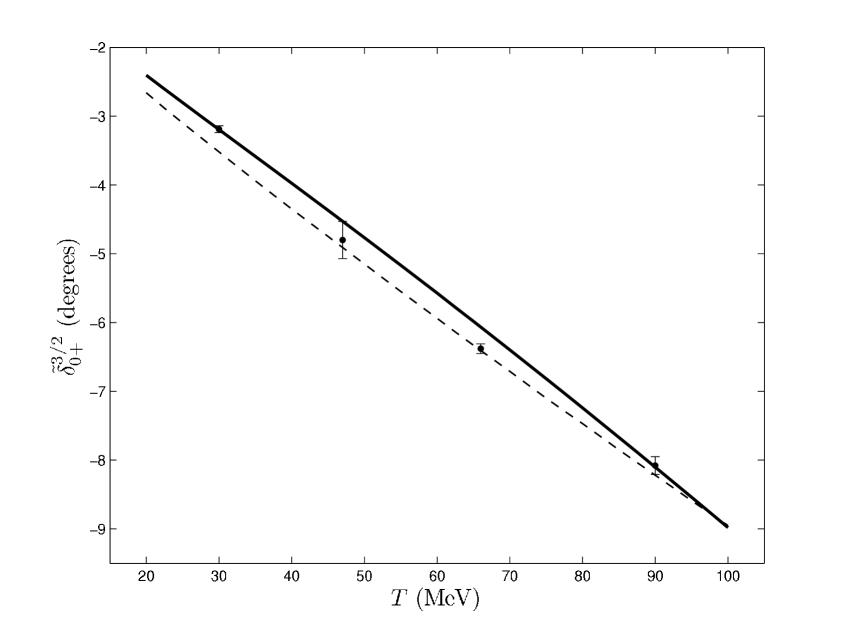
Figure 1: The em-modified hadronic phase shift $\tilde{\delta}_{0+}^{3/2}$

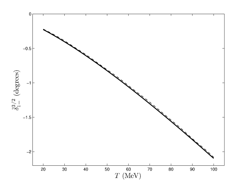
Figure 2: The em-modified hadronic phase shift $\tilde{\delta}_{1-}^{3/2}$

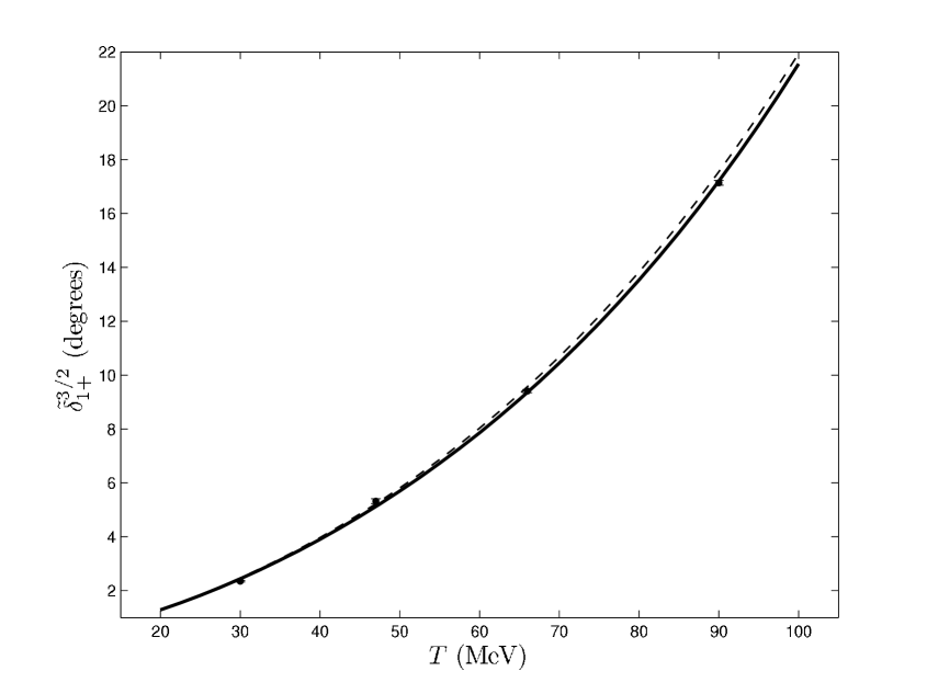
Figure 3: The em-modified hadronic phase shift $\tilde{\delta}_{1+}^{3/2}$

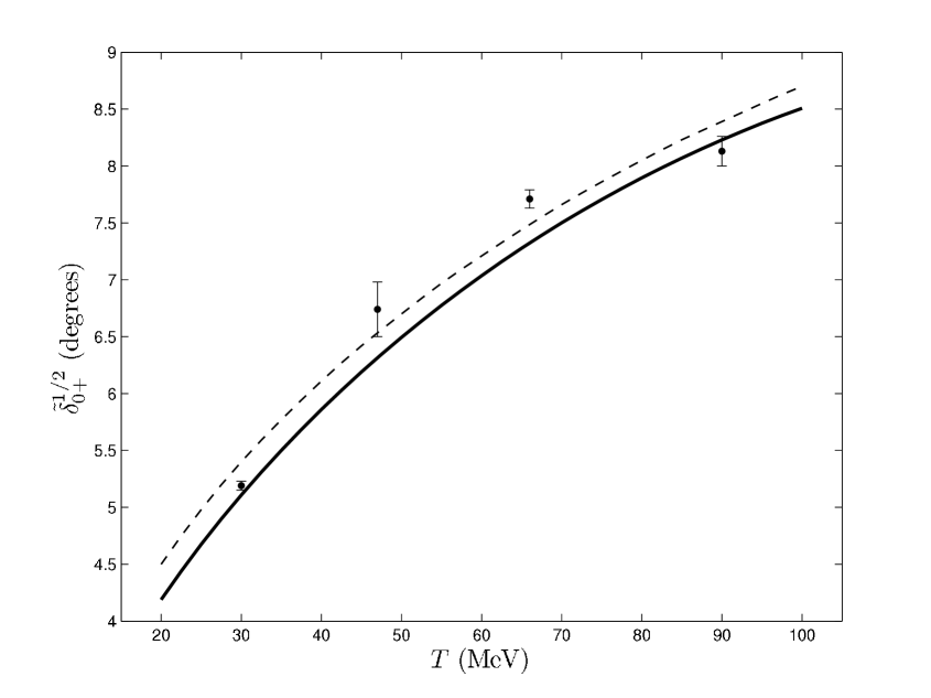
Figure 4: The em-modified hadronic phase shift $\tilde{\delta}_{0+}^{1/2}$

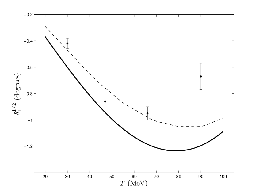
Figure 5: The em-modified hadronic phase shift $\tilde{\delta}_{1-}^{1/2}$

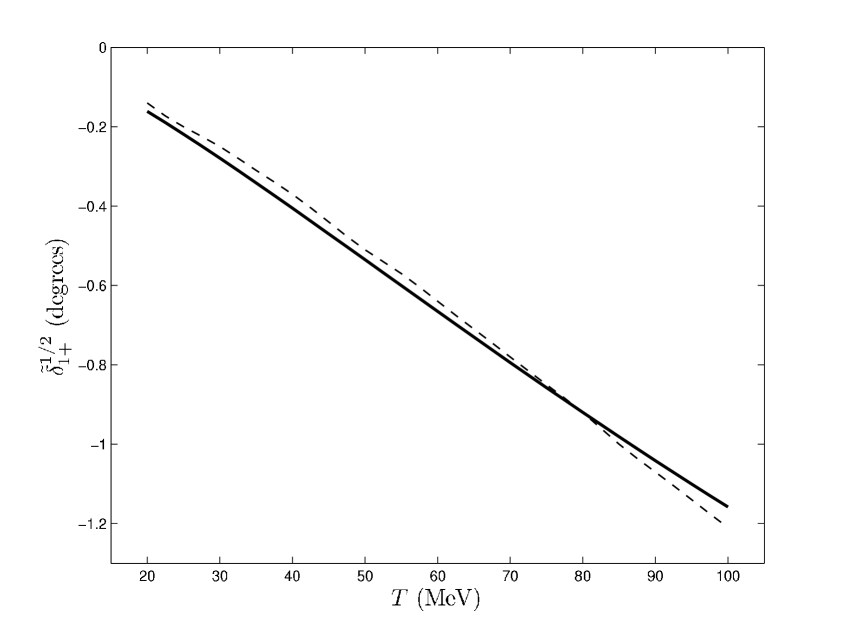
Figure 6: The em-modified hadronic phase shift $\tilde{\delta}_{1+}^{1/2}$

The final $s$- and $p$-wave em-modified hadronic phase shifts, from the model fit to the combined truncated elastic-scattering database, are given in Table 5, in $5$ MeV intervals from $20$ to $100$ MeV. These hadronic phase shifts are also shown in Figs. 1-6, together with the current GWU solution [5] and their four single-energy values (whenever available).

It is evident from Figs. 1 and 4 that our values of the $s$-wave hadronic phase shifts $\tilde{\delta}_{0+}^{3/2}$ and $\tilde{\delta}_{0+}^{1/2}$ differ significantly from the GWU results. Our values of $\tilde{\delta}_{0+}^{3/2}$ are less negative, but converge towards the GWU values as the energy approaches $100$ MeV. Interestingly, the GWU single-energy results at $30$ and $90$ MeV agree with our results. For $\tilde{\delta}_{0+}^{1/2}$, our values are consistently smaller, with a slight convergence towards $100$ MeV. Once again, the GWU single-energy results at $30$ and $90$ MeV agree with ours, but the ones at $47$ and $66$ MeV do not. For the $p$-wave hadronic phase shifts $\tilde{\delta}_{1-}^{3/2}$, $\tilde{\delta}_{1+}^{3/2}$ and $\tilde{\delta}_{1+}^{1/2}$, inspection of Figs. 2, 3 and 6 shows that there is good agreement between the two solutions. The significant difference in the $p$-wave part of the interaction occurs for $\tilde{\delta}_{1-}^{1/2}$. Our values are clearly considerably lower at all energies and the single-energy GWU results are a long way from ours except at $47$ MeV. The differences between our results for the hadronic phase shifts and those of GWU are not due to the improved stage 1 EM corrections which we have used. In fact, the exact values of the EM corrections used have very little effect on the output of the PSA. The differences are due almost entirely to the method we have used, restricting the data being analysed to $T\leq 100$ MeV and freely floating the data from only three experiments, thus respecting as far as possible the measurements as they have been published.

We conclude this section with a discussion of the measurements of Ref. [34] which have not been included in our database. Using our phase-shift output, we have created Monte-Carlo predictions for the analysing power corresponding to each of their $28$ experimental points. For the three experimental data sets, the resulting values of $\chi^{2}_{min}$ are $12.72$, $7.41$ and $15.87$, for $12$, $6$ and $10$ degrees of freedom. The values of the scale factor for the three sets (in the same order) are $1.0079$, $0.9718$ and $1.0360$. It is evident, not only that all the data points satisfy the acceptance criterion which was applied to the full $\pi^{+}p$ and $\pi^{-}p$ databases (see Section 4), but also that our hadronic phase shifts reproduce the data of Ref. [34] very well; even the data set which is reproduced least well corresponds to a p-value of $0.1035$. Our conclusion is that, even if the data of Ref. [34] were in a form which could easily enable their inclusion in our database, the impact on our results would have been negligible. For one thing, the data are very well reproduced by our present solution; for another, they correspond to about $4.2\%$ of the combined truncated elastic-scattering database which we have used for our analysis.

7 Analysis of the $\pi^{-}p$ charge-exchange data and the violation of isospin invariance

For reasons given in Section 1, our PSA was based on the elastic-scattering data only. The EM corrections of Refs. [1, 2] were applied and the hadronic part of each scattering amplitude was parameterised in a framework of formal isospin invariance, leading to the extraction of the six $s$- and $p$-wave em-modified hadronic phase shifts $\tilde{\delta}$. Because of the residual EM effects, it is not very surprising that there is evidence for the violation of isospin invariance at the em-modified level [6, 7]. In Ref. [6], it was shown that the violation of isospin invariance appears mainly in the $s$-wave amplitude, with some effect also present in the no-spin-flip $p$ wave. We will now strengthen the evidence in Refs. [6, 7], by using the output of our PSA of the elastic-scattering data to attempt to reproduce the measurements on the CX reaction $\pi^{-}p\to\pi^{0}n$.

There is an extensive database of CX measurements below $100$ MeV. The modern measurements of the DCS come from four experiments, namely FITZGERALD86 [44], FRLEŽ98 [45], ISENHOWER99 [46] and SADLER04 [47]. The FITZGERALD86 data comprise measurements of the DCS close to $0^{\circ}$ at seven energies, from $32.5$ to $63.2$ MeV; only their direct measurements were used here (their extrapolated values to $0^{\circ}$ were not taken into account). FRLEŽ98 measured the DCS at $27.5$ MeV, at six angles between $4.7^{\circ}$ and $50.9^{\circ}$. ISENHOWER99 measured the DCS at $10.6$, $20.6$ and $39.4$ MeV; the groups of points near $0^{\circ}$, $90^{\circ}$ and $180^{\circ}$ have independent beam normalisations, thus leading to eight independent data sets. SADLER04 made detailed measurements of the DCS at $63.9$, $83.5$ and $94.6$ MeV. These four experiments share a common characteristic: they all measured the CX DCS in the forward hemisphere. We will now explain why they are expected to be more conclusive than the rest of the experiments on the issue of isospin invariance. The main contributions to the CX scattering amplitude in the low-energy region come from the real parts of the $s$ and $p$ waves. Taking into account the opposite signs of these contributions, the two main components of the scattering amplitude almost cancel each other in the forward direction around $40$ MeV, thus enabling small effects to show up. The destructive-interference phenomenon acts like a magnifying glass, probing the smaller components in the $\pi N$ dynamics. Note that the two studies [6, 7] of the isospin-invariance violation did not have the results in Refs. [45]-[47] available to them.

There are a number of additional CX data sets which, for various reasons, are not expected to contribute to the discussion of the isospin-invariance violation. a) The experiment of DUCLOS73 [48] measured the DCS near $180^{\circ}$ at $22.6$, $32.9$ and $42.6$ MeV. Apart from the large statistical uncertainties of these three data points (which, according to Eq. (26), bring the scale factors closer to $1$), the contributions of the $s$ and $p$ waves add in the backward hemisphere (constructive interference), thus masking any small effects which might be present in the $\pi N$ dynamics at these energies. b) There are two similar experiments, SALOMON84 [49] and BAGHERI88 [50], whose output consisted of the first three coefficients in a Legendre expansion of the DCS at six energies between $27.4$ and $91.7$ MeV. Even if the correlation matrices, corresponding to the different energies where the measurements were taken, could be found in these papers, the raw DCS data could not be reconstructed; one could obtain only the fitted values, but no knowledge of how these fitted values compare with the measured values of the DCS. c) There is a measurement of the total cross section for the CX reaction at $90.9$ MeV from the experiment of BUGG71 [51]. d) Finally, there are measurements of the analysing power at $100$ MeV (STAŠKO93 [52]) and $98.1$ MeV (GAULARD99 [53]). In cases (c) and (d) above, the energy used was high; additionally, in case (d), the sensitivity of the analysing power to the effect being investigated in this section is questionable.

The full database for the CX reaction consists of $31$ data sets, containing $159$ data points. In cases where a normalisation uncertainty was not properly reported, we had to assign realistic normalisation errors by comparison with those quoted for other experiments. The precise details are not important.

The first step was to check the consistency of the CX data in the same way as we have done for the $\pi^{-}p$ elastic-scattering database. The $I=3/2$ amplitudes were fixed from the final fit to the $\pi^{+}p$ database of Table 1 and the seven parameters for the $I=1/2$ amplitudes were varied in order to optimise the description of the CX data via the minimisation of the Arndt-Roper function. The minimum value of $\chi^{2}$ was $154.9$ for $152$ degrees of freedom (with p-value equal to $0.42$); no doubtful data sets or individual data points could be found. On the other hand, when we attempted to reproduce the CX database using the output of the fit to the combined truncated elastic-scattering data, the value of $\chi^{2}$ jumped to an enormous $508.9$. The DCS of Refs. [44]-[48] and the total cross section of Ref. [51], $131$ data points in total, contribute $471.2$ units to the overall $\chi^{2}$; as previously mentioned, it is in the DCS measurements in the forward hemisphere that the effect is expected to show up best. The analysing-power measurements of Refs. [52, 53] are reproduced well. With the exception of the data set at $45.6$ MeV, the indirect data of Refs. [49, 50] are also well reproduced.

The conclusion is that the CX database cannot be satisfactorily reproduced from the PSA of the $\pi^{\pm}p$ elastic-scattering data which used a framework of formal isospin invariance. This is conclusive evidence that isospin invariance is violated at the em-modified hadronic level, thus corroborating the findings of Refs. [6, 7] which were based on a significantly smaller CX database. The predictions, based on the output from the PSA of the elastic-scattering data, seriously underestimate the measured CX cross sections.

We content ourselves here with this clear evidence for the violation of isospin invariance at the em-modified level. What is still needed is a new PSA, of the combined $\pi^{+}p$ elastic-scattering and $\pi^{-}p$ CX databases, using the same model as before. The output will consist of $I=3/2$ hadronic phase shifts, which one expects to be very close to those given in Section 6, and new ‘I = 1/2’ hadronic phase shifts, which will be substantially different from those given in Section 6. The differences will be able to make more precise the conclusions of Ref. [6], on the size of the violation of isospin invariance in the $s$ wave and the two $p$ waves. Further, comparison of the values of the $s$-wave threshold parameter for $\pi^{-}p$ CX scattering, obtained from the new PSA and from the width of the $1s$ level of pionic hydrogen, will provide further information on the reliability of the $\pi^{+}p$ elastic-scattering and $\pi^{-}p$ CX databases.

8 Discussion

In the present paper, we have reported the results of a PSA of the $\pi^{\pm}p$ elastic-scattering data for $T\leq 100$ MeV using the recently obtained EM corrections of Refs. [1, 2]; the analysis was performed with a hadronic interaction described within a framework of formal isospin invariance. We found that it was possible to obtain self-consistent databases by removing the measurements of only two $\pi^{+}p$ data sets and one $\pi^{-}p$ set, as well as a very small number of single data points; the removal of these outliers resulted in enormous reductions in the minimum value of $\chi^{2}$ for the separate fits to the two elastic-scattering databases.

The $\pi N$ model of Ref. [14], based on s- and u-channel diagrams with $N$ and $\Delta$ in the intermediate states, and $\sigma$ and $\rho$ t-channel exchanges, was subsequently fitted to the elastic-scattering database obtained after the removal of the outliers. The model-parameter values showed an impressive stability when subjected to different criteria for the rejection of experiments (see Table 3); we finally adopted the criterion which removes the smallest amount of experimental data, and adjusted the output uncertainties in such a way as to take account of the quality of the fit. Our final result for the pseudovector $\pi NN$ coupling constant is $0.0733\pm 0.0014$. Our $s$- and $p$-wave em-modified hadronic phase shifts are given in Table 5. Big differences in the $s$-wave part of the interaction were found when comparing our hadronic phase shifts with the current GWU solution [5] (see Figs. 1 and 4); there is general agreement in the $p$ waves, except for the $\tilde{\delta}_{1-}^{1/2}$ hadronic phase shift. We observed that these differences come from our decision to restrict the analysis to data for $T\leq 100$ MeV, and pointed out the apparent mismatch between this data and data at higher energies. We also showed that there is a serious discrepancy between our $s$-wave scattering lengths and the value of the $s$-wave threshold parameter for $\pi^{-}p$ elastic scattering obtained from pionic hydrogen. There is no simple way to account for these differences, and serious questions about the low-energy elastic-scattering database remain unanswered.

We showed that the experimental results for the CX reaction $\pi^{-}p\to\pi^{0}n$ cannot be reproduced using the output from the PSA of the elastic-scattering data; this inability corroborates the findings of Refs. [6, 7] concerning the violation of isospin invariance in the em-modified hadronic $\pi N$ interaction at low energies. We pointed out in Section 1 the need for stage 2 EM corrections (to remove the EM effects in the hadronic interaction) to be calculated, first for all threshold parameters, and subsequently for the analysis of scattering data at nonzero energies for all three reaction types. Until such corrections exist, it is necessary to use the existing stage 1 corrections to analyse the available scattering data, as we have done.

Note added in proof

While this work was being reviewed, additional CX data appeared [54], namely values of the total cross section at eighteen energies, nine of them below $100$ MeV. The measurements below $100$ MeV are reproduced very well by our phase-shift solution.

Table 1:

The data sets comprising the truncated database for $\pi^{+}p$ elastic scattering, the pion laboratory kinetic energy $T$ (in MeV), the number of degrees of freedom $(NDF)_{j}$ for each set, the scale factor $z_{j}$ which minimises $\chi_{j}^{2}$, the values of $(\chi_{j}^{2})_{min}$ and the p-value for each set.

Data set	$T$	$(NDF)_{j}$	$z_{j}$	$\chi_{j}^{2}$	$p$	Comments
AULD79	47.9	11	1.0101	16.4245	0.1261
RITCHIE83	65.0	8	1.0443	17.4019	0.0262
RITCHIE83	72.5	10	1.0061	4.7745	0.9057
RITCHIE83	80.0	10	1.0297	19.3025	0.0366
RITCHIE83	95.0	10	1.0315	12.4143	0.2583
FRANK83	29.4	28	0.9982	17.4970	0.9381
FRANK83	49.5	28	1.0402	34.3544	0.1894
FRANK83	69.6	27	0.9290	23.3002	0.6688
FRANK83	89.6	27	0.8618	29.1920	0.3517
BRACK86	66.8	4	0.8914	2.5020	0.6443	freely floated
BRACK86	86.8	8	0.9387	16.6304	0.0342	freely floated
BRACK86	91.7	5	0.9734	11.9985	0.0348
BRACK86	97.9	5	0.9714	7.5379	0.1836
BRACK88	66.8	6	0.9469	11.2438	0.0811
BRACK88	66.8	6	0.9561	9.8897	0.1294
WIEDNER89	54.3	19	0.9851	14.7822	0.7363
BRACK90	30.0	6	1.0946	17.7535	0.0069
BRACK90	45.0	8	1.0055	7.8935	0.4439
BRACK95	87.1	8	0.9733	13.3922	0.0991
BRACK95	98.1	8	0.9820	14.8872	0.0614
JORAM95	45.1	9	0.9548	22.2169	0.0082	one point removed
JORAM95	68.6	9	1.0503	8.8506	0.4512
JORAM95	32.2	19	1.0087	23.7410	0.2063	one point removed
JORAM95	44.6	18	0.9503	29.8018	0.0394	two points removed
SEVIOR89	98.0	6	1.0178	5.3726	0.4970

Table 1 continued

Data set	$T$	$(NDF)_{j}$	$z_{j}$	$\chi_{j}^{2}$	$p$	Comments
WIESER96	68.34	3	0.8945	2.4732	0.4802
WIESER96	68.34	4	0.9252	3.6315	0.4582
KRISS97	39.8	1	1.0121	1.7222	0.1894
KRISS97	40.5	1	1.0017	0.1400	0.7083
KRISS97	44.7	1	1.0020	0.0415	0.8385
KRISS97	45.3	1	1.0025	0.0518	0.8200
KRISS97	51.1	1	1.0240	3.3209	0.0684
KRISS97	51.7	1	1.0024	0.0397	0.8421
KRISS97	54.8	1	1.0068	0.1376	0.7107
KRISS97	59.3	1	1.0252	1.2497	0.2636
KRISS97	66.3	2	1.0501	4.0858	0.1297
KRISS97	66.8	2	1.0075	0.5897	0.7446
KRISS97	80.0	1	1.0142	0.3704	0.5428
KRISS97	89.3	1	1.0079	0.2849	0.5935
KRISS97	99.2	1	1.0550	4.1084	0.0427
FRIEDMAN99	45.0	1	1.0423	2.1509	0.1425
FRIEDMAN99	52.1	1	1.0172	0.2461	0.6198
FRIEDMAN99	63.1	1	1.0364	0.4918	0.4831
FRIEDMAN99	67.45	2	1.0524	1.2636	0.5316
FRIEDMAN99	71.5	2	1.0501	0.8458	0.6551
FRIEDMAN99	92.5	2	1.0429	0.5860	0.7460
CARTER71	71.6	1	1.0933	2.7422	0.0977
CARTER71	97.4	1	1.0495	0.6856	0.4077
PEDRONI78	72.5	1	1.0125	0.1416	0.7067
PEDRONI78	84.8	1	1.0319	0.3443	0.5574
PEDRONI78	95.1	1	1.0230	0.2024	0.6528
PEDRONI78	96.9	1	1.0166	0.1305	0.7179

Table 2:

The data sets comprising the truncated database for $\pi^{-}p$ elastic scattering, the pion laboratory kinetic energy $T$ (in MeV), the number of degrees of freedom $(NDF)_{j}$ for each set, the scale factor $z_{j}$ which minimises $\chi_{j}^{2}$, the values of $(\chi_{j}^{2})_{min}$ and the p-value for each set.

Data set	$T$	$(NDF)_{j}$	$z_{j}$	$\chi_{j}^{2}$	$p$	Comments
FRANK83	29.4	28	0.9828	31.1504	0.3104
FRANK83	49.5	28	1.1015	29.4325	0.3908
FRANK83	69.6	27	1.0931	27.0824	0.4594
FRANK83	89.6	27	0.9467	24.7108	0.5907
BRACK86	66.8	5	0.9965	14.3569	0.0135
BRACK86	86.8	5	1.0032	1.3478	0.9299
BRACK86	91.7	5	0.9964	3.0272	0.6958
BRACK86	97.9	5	1.0003	5.8335	0.3228
WIEDNER89	54.3	18	1.1563	23.5094	0.1718	one point removed, freely floated
BRACK90	30.0	5	1.0215	5.2577	0.3853
BRACK90	45.0	9	1.0541	12.2642	0.1988
BRACK95	87.5	6	0.9816	10.7547	0.0963
BRACK95	98.1	7	1.0067	8.8236	0.2656	one point removed
JORAM95	32.7	4	0.9937	3.7670	0.4385
JORAM95	32.7	2	0.9533	5.6487	0.0593
JORAM95	45.1	4	0.9562	12.0551	0.0169
JORAM95	45.1	3	0.9459	9.4574	0.0238
JORAM95	68.6	7	1.0841	14.8484	0.0380
JORAM95	68.6	3	1.0281	2.3391	0.5051
JORAM95	32.2	20	1.0587	20.8026	0.4088
JORAM95	44.6	20	0.9421	30.5855	0.0609
JANOUSCH97	43.6	1	1.0427	0.1745	0.6762
JANOUSCH97	50.3	1	1.0348	0.1418	0.7065
JANOUSCH97	57.3	1	1.0830	4.5260	0.0334
JANOUSCH97	64.5	1	1.0152	0.0153	0.9015
JANOUSCH97	72.0	1	1.3059	4.8803	0.0272

Table 2 continued

Data set	$T$	$(NDF)_{j}$	$z_{j}$	$\chi_{j}^{2}$	$p$	Comments
ALDER83	98.0	6	1.0338	5.1831	0.5206
SEVIOR89	98.0	5	0.9890	1.6659	0.8932
HOFMAN98	86.8	11	1.0015	6.0355	0.8710
PATTERSON02	57.0	10	0.9377	11.2510	0.3383
PATTERSON02	66.9	9	0.9986	4.5388	0.8725
PATTERSON02	66.9	10	0.9502	17.0121	0.0741
PATTERSON02	87.2	11	0.9827	8.5353	0.6647
PATTERSON02	87.2	11	0.9932	5.2523	0.9183
PATTERSON02	98.0	12	0.9964	7.0659	0.8532

Table 3:

The values of the seven parameters of the $\pi N$ model obtained from fits to the combined truncated elastic-scattering database, chosen using four different values of $\mathrm{p}_{min}$ (the significance level for rejection of data points). The uncertainties correspond to the fit with $\mathrm{p}_{min}=0.0027$.

	0.0027	0.01	0.05	0.10	error
$G_{\sigma}(GeV^{-2})$	26.76	26.72	26.72	27.04	0.85
$K_{\sigma}$	0.011	0.009	0.013	0.020	0.036
$G_{\rho}(GeV^{-2})$	55.07	55.04	55.05	55.69	0.61
$K_{\rho}$	0.68	0.62	0.63	0.84	0.40
$g_{\pi NN}$	12.91	12.90	12.90	12.94	0.12
$g_{\pi N\Delta}$	29.70	29.71	29.60	29.64	0.27
$Z$	-0.528	-0.530	-0.521	-0.510	0.059

Table 4:

The correlation matrix for the seven parameters of the $\pi N$ model, for the fit to the combined truncated elastic-scattering database corresponding to $\mathrm{p}_{min}=0.0027$.

	$G_{\sigma}$	$K_{\sigma}$	$G_{\rho}$	$K_{\rho}$	$g_{\pi NN}$	$g_{\pi N\Delta}$	$Z$
$G_{\sigma}$	1.0000	0.4762	-0.0903	-0.0288	0.1036	-0.1606	-0.1928
$K_{\sigma}$	0.4762	1.0000	0.7539	0.8226	0.9011	-0.9343	0.7502
$G_{\rho}$	-0.0903	0.7539	1.0000	0.9051	0.9058	-0.8507	0.9002
$K_{\rho}$	-0.0288	0.8226	0.9051	1.0000	0.9529	-0.9290	0.9510
$g_{\pi NN}$	0.1036	0.9011	0.9058	0.9529	1.0000	-0.9499	0.9239
$g_{\pi N\Delta}$	-0.1606	-0.9343	-0.8507	-0.9290	-0.9499	1.0000	-0.9031
$Z$	-0.1928	0.7502	0.9002	0.9510	0.9239	-0.9031	1.0000

Table 5:

The values of the six $s$- and $p$-wave em-modified hadronic phase shifts (in degrees) from the PSA of the combined truncated elastic-scattering database.

$T(MeV)$	$\tilde{\delta}_{0+}^{3/2}$	$\tilde{\delta}_{1-}^{3/2}$	$\tilde{\delta}_{1+}^{3/2}$	$\tilde{\delta}_{0+}^{1/2}$	$\tilde{\delta}_{1-}^{1/2}$	$\tilde{\delta}_{1+}^{1/2}$
20	-2.41(3)	-0.23(0)	1.28(1)	4.19(3)	-0.37(1)	-0.16(0)
25	-2.80(4)	-0.31(1)	1.82(1)	4.67(3)	-0.49(1)	-0.22(1)
30	-3.19(4)	-0.40(1)	2.44(2)	5.11(3)	-0.60(1)	-0.28(1)
35	-3.58(4)	-0.50(1)	3.13(2)	5.50(3)	-0.71(2)	-0.34(1)
40	-3.98(4)	-0.61(1)	3.90(2)	5.86(3)	-0.81(2)	-0.41(1)
45	-4.37(4)	-0.71(2)	4.76(2)	6.19(3)	-0.91(2)	-0.47(1)
50	-4.77(4)	-0.82(2)	5.70(2)	6.49(4)	-0.99(3)	-0.54(2)
55	-5.17(4)	-0.94(2)	6.73(3)	6.78(4)	-1.07(3)	-0.60(2)
60	-5.57(4)	-1.06(3)	7.86(3)	7.04(4)	-1.13(3)	-0.67(2)
65	-5.98(4)	-1.18(3)	9.10(3)	7.28(5)	-1.18(4)	-0.73(2)
70	-6.40(4)	-1.30(3)	10.45(3)	7.50(5)	-1.21(4)	-0.79(3)
75	-6.82(5)	-1.43(4)	11.92(3)	7.71(6)	-1.23(5)	-0.86(3)
80	-7.24(5)	-1.56(4)	13.53(4)	7.90(6)	-1.24(5)	-0.92(3)
85	-7.67(6)	-1.69(5)	15.29(5)	8.07(7)	-1.22(6)	-0.98(4)
90	-8.10(7)	-1.82(5)	17.20(6)	8.23(7)	-1.20(6)	-1.04(4)
95	-8.54(8)	-1.96(6)	19.29(7)	8.38(8)	-1.15(7)	-1.10(4)
100	-8.98(8)	-2.10(6)	21.56(9)	8.51(9)	-1.09(7)	-1.16(5)

from the present work (solid curve) and from the current GWU solution [5] (dashed curve). The four single-energy points of Ref. [5], at $30,47,66$ and $90$ MeV, are also shown.

from the present work (solid curve) and from the current GWU solution [5] (dashed curve).

from the present work (solid curve) and from the current GWU solution [5] (dashed curve). The four single-energy points of Ref. [5], at $30,47,66$ and $90$ MeV, are also shown.

from the present work (solid curve) and from the current GWU solution [5] (dashed curve). The four single-energy points of Ref. [5], at $30,47,66$ and $90$ MeV, are also shown.

from the present work (solid curve) and from the current GWU solution [5] (dashed curve). The four single-energy points of Ref. [5], at $30,47,66$ and $90$ MeV, are also shown.

from the present work (solid curve) and from the current GWU solution [5] (dashed curve).

References

- [1] A. Gashi, E. Matsinos, G.C. Oades, G. Rasche, W.S. Woolcock, Nucl. Phys. A 686 (2001) 447.
- [2] A. Gashi, E. Matsinos, G.C. Oades, G. Rasche, W.S. Woolcock, Nucl. Phys. A 686 (2001) 463.
- [3] B. Tromborg, S. Waldenstrøm, I. Øverbø, Phys. Rev. D 15 (1977) 725.
- [4] R. Koch, E. Pietarinen, Nucl. Phys. A336 (1980) 331; R. Koch, Nucl. Phys. A 448 (1986) 707.
- [5] R.A. Arndt, W.J. Briscoe, R.L. Workman, I.I. Strakovsky, SAID on-line program, at http://gwdac.phys.gwu.edu [status: 27.06.05].
- [6] W.R. Gibbs, Li Ai, W.B. Kaufmann, Phys. Rev. Lett. 74 (1995) 3740.
- [7] E. Matsinos, Phys. Rev. C 56 (1997) 3014.
- [8] H.-Ch. Schröder et al., Eur. Phys. J. C 21 (2001) 473.
- [9] M. Hennebach, Ph.D. dissertation, Universität zu Köln, 2003.
- [10] J. Gasser, M.A. Ivanov, E. Lipartia, M. Mojžiš and A. Rusetsky, Eur. Phys. J. C26 (2002) 13.
- [11] N. Fettes, U.-G. Meißner, Nucl. Phys. A 693 (2001) 693.
- [12] N. Fettes, E. Matsinos, Phys. Rev. C 55 (1997) 464.
- [13] R.A. Arndt, L.D. Roper, Nucl. Phys. B 50 (1972) 285.
- [14] P.F.A. Goudsmit, H.J. Leisi, E. Matsinos, B.L. Birbrair, A.B. Gridnev, Nucl. Phys. A 575 (1994) 673; more references on the development of the model may be found at http://people.web.psi.ch/matsinos/0_home.htm.
- [15] E.G. Auld et al., Can. J. Phys. 57 (1979) 73.
- [16] B.G. Ritchie et al., Phys. Lett. B 125 (1983) 128.
- [17] J.S. Frank et al., Phys. Rev. D 28 (1983) 1569.
- [18] J.T. Brack et al., Phys. Rev. C 34 (1986) 1771.
- [19] J.T. Brack et al., Phys. Rev. C 38 (1988) 2427.
- [20] U. Wiedner et al., Phys. Rev. D 40 (1989) 3568.
- [21] J.T. Brack et al., Phys. Rev. C 41 (1990) 2202.
- [22] J.T. Brack et al., Phys. Rev. C 51 (1995) 929.
- [23] Ch. Joram et al., Phys. Rev. C 51 (1995) 2144; Ch. Joram et al., ibid. C 51 (1995) 2159.
- [24] M.E. Sevior et al., Phys. Rev. C 40 (1989) 2780.
- [25] R. Wieser et al., Phys. Rev. C 54 (1996) 1930.
- [26] B.J. Kriss et al., Newsletter 12 (1997) 20; B.J. Kriss et al., Phys. Rev. C 59 (1999) 1480.
- [27] E. Friedman, Newsletter 15 (1999) 37.
- [28] A.A. Carter, J.R. Williams, D.V. Bugg, P.J. Bussey, D.R. Dance, Nucl. Phys. B 26 (1971) 445.
- [29] E. Pedroni et al., Nucl. Phys. A 300 (1978) 321.
- [30] M. Janousch et al., Phys. Lett. B 414 (1997) 237.
- [31] J.C. Alder et al., Phys. Rev. D 27 (1983) 1040.
- [32] G.J. Hofman et al., Phys. Rev. C 58 (1998) 3484.
- [33] J.D. Patterson et al., Phys. Rev. C 66 (2002) 025207.
- [34] R. Meier et al., Phys. Lett. B 588 (2004) 155.
- [35] T.E.O. Ericson, W. Weise, Pions and Nuclei (Clarendon Press, Oxford, 1988), p. 31.
- [36] S. Eidelman et al. (Particle Data Group), Phys. Lett. B 592 (2004) 1.
- [37] T.E.O. Ericson et al., Phys. Rev. Lett. 75 (1995) 1046.
- [38] W. Jaus, W.S. Woolcock, Nucl. Phys. A 608 (1996) 389.
- [39] R. Timmermans, Th.A. Rijken, J.J. de Swart, Phys. Rev. C 50 (1994) 48.
- [40] F. Bradamante, A. Bressan, M. Lamanna, A. Martin, Phys. Lett. B 343 (1995) 431.
- [41] M.G. Olsson, E.T. Osypowski, Nucl. Phys. B 101 (1975) 136.
- [42] V. Bernard, T.R. Hemmert, U.-G. Meißner, Phys. Lett. B 565 (2003) 137.
- [43] G.C. Oades, G. Rasche, W.S. Woolcock, E. Matsinos, A. Gashi, in preparation.
- [44] D.H. Fitzgerald et al., Phys. Rev. C 34 (1986) 619.
- [45] E. Frlež et al., Phys. Rev. C 57 (1998) 3144.
- [46] L.D. Isenhower et al., Newsletter 15 (1999) 292.
- [47] M.E. Sadler et al., Phys. Rev. C 69 (2004) 055206.
- [48] J. Duclos et al., Phys. Lett. B 43 (1973) 245.
- [49] M. Salomon, D.F. Measday, J-M. Poutissou, B.C. Robertson, Nucl. Phys. A 414 (1984) 493.
- [50] A. Bagheri et al., Phys. Rev. C 38 (1988) 885.
- [51] D.V. Bugg et al., Nucl. Phys. B 26 (1971) 588.
- [52] J.C. Staško, Ph.D. dissertation, University of New Mexico, 1993.
- [53] C.V. Gaulard et al., Phys. Rev. C 60 (1999) 024604.
- [54] J. Breitschopf et al., Phys. Lett. B, in print; preprint nucl-ex/0605017.