LPTHE-P06-04

FASTJET: A CODE FOR FAST $k_{t}$ CLUSTERING, AND MORE 

Two main classes of jet clustering algorithms, cone and $k_{t}$, are briefly discussed. It is argued that the former can be often cumbersome to define and implement, and difficult to analyze in terms of its behaviour with respect to soft and collinear emissions. The latter, on the other hand, enjoys a very simple definition, and can be easily shown to be infrared and collinear safe. Its single potential shortcoming, a computational complexity believed to scale like the number of particles to the cube ($N^{3}$), is overcome by introducing a new geometrical algorithm that reduces it to $N\ln N$. A practical implementation of this approach to $k_{t}$-clustering, FastJet, is shown to be orders of magnitude faster than all other present codes, opening the way to the use of $k_{t}$-clustering even in highly populated heavy ion events.

High energy events are often studied in terms of jets. While a “jet” is in principle just a roughly collimated bunch of particles flying in the same direction, it takes of course a more careful definition to make it a tool for an accurate analysis of QCD. In particular, in order to be able to compare the experimentally observed jets to theoretical predictions, one must ensure that the measured quantity is “soft and collinear safe”, meaning that the addition of a soft or a collinear parton does not change its value. Only for this type of quantity can higher order calculations in QCD give sensible results.

While jets have been discussed since the beginning of the ’70s, the first modern definition of a soft and collinear safe jet is due to Sterman and Weinberg $\!{}^{{\bf?}}$. Their jets, whose definition was originally formulated for $e^{+}e^{-}$ collisions, were of a kind which became successively known as ‘cone-type’. They have been successively extended to hadronic collisions, where cone-type jets are based on identifying energy-flow into cones in (pseudo)rapidity $\eta=-\ln\tan\theta/2$ and azimuth $\phi$, together with various steps of iteration, merging and splitting of the cones to obtain the final jets. The freedom in the details of the clustering procedure has led to a number of definitions of cone-type jet clustering algorithms, many of them currently used at the Tevatron and in preliminary studies of LHC analyses $\!{}^{{\bf?}}$. However, cone jet-finders tend to be rather complex: different experiments have used different variants (some of them infrared unsafe), and it is often difficult to know exactly which jet-finder to use in theoretical comparisons.

Partly in order to overcome these difficulties, at the beginning of the ’90s cluster-type jet-finders where proposed. They are generally based on successive pair-wise recombination of particles, have simple definitions and are all infrared safe . The most widely used of them is the $k_{t}$ jet-finder $\!{}^{{\bf?}}$, defined below. Among its physics advantages are (a) that it purposely mimics a walk backwards through the QCD branching sequence, which means that reconstructed jets naturally collect most of the particles radiated from an original hard parton, giving better particle mass measurements $\!{}^{{\bf?},{\bf?}}$ and gaps-between-jets identification $\!{}^{{\bf?}}$ (of relevance to Higgs searches); and (b) it allows one to decompose a jet into constituent subjets, which is useful for identifying decay products of fast-moving heavy particles (see e.g. $\!{}^{{\bf?}}$) and various QCD studies. This has led to the widespread adoption of the $k_{t}$ jet-finder in the LEP ($e^{+}e^{-}$ collisions) and HERA ($ep$) communities.

The $k_{t}$ jet-finder, in the longitudinally invariant formulation suitable for hadron colliders, is defined as follows.

The $k_{t}$ jet-finder

1. For each pair of particles $i$, $j$ work out the $k_{t}$ distance $d_{ij}=\min(k_{ti}^{2},{k_{tj}^{2}})R_{ij}^{2}$ with $R_{ij}^{2}=(\eta_{i}-\eta_{j})^{2}+(\phi_{i}-\phi_{j})^{2}$, where $k_{ti}$, $\eta_{i}$ and $\phi_{i}$ are the transverse momentum, rapidity and azimuth of particle $i$; for each parton $i$ also work out the beam distance $d_{iB}=k_{ti}^{2}$. 2. Find the minimum $d_{\min}$ of all the $d_{ij},d_{iB}$. If $d_{\min}$ is a $d_{ij}$ merge particles $i$ and $j$ into a single particle, summing their four-momenta (alternative recombination schemes are possible); if it is a $d_{iB}$ then declare particle $i$ to be a final jet and remove it from the list. 3. Repeat from step 1 until no particles are left.

One apparent drawback of this algorithm is its computational complexity, originally believed to scale like $N^{3}$, $N$ being the number of particles to be clustered. This complexity leads to concrete implementations which become slow as $N$ grows, making the use of $k_{t}$-clustering impractical in environments where large numbers of particles are produced in the final state, like hadron-hadron or, even more spectacularly, ion-ion collisions.

We show here that this computational complexity can in fact be reduced to $N\ln N$, opening the way to a much more widespread use of the $k_{t}$ jet-finder $\!{}^{{\bf?}}$.

To obtain a better algorithm we isolate the geometrical aspects of the problem, with the help of the following observation (see $\!{}^{{\bf?}}$ for its proof): If $i$, $j$ form the smallest $d_{ij}$, and $k_{ti}<k_{tj}$, then $R_{ij}<R_{i\ell}$ for all $\ell\neq j$, i.e. $j$ is the geometrical nearest neighbour of particle $i$.

This means that if we can identify each particle’s geometrical nearest neighbour (in terms of the geometrical $R_{ij}$ distance), then we need not construct a size-$N^{2}$ table of $d_{ij}=\min(k_{ti}^{2},{k_{tj}^{2}})R_{ij}^{2}$, but only the size-$N$ array, $d_{i{{\cal G}\!}_{i}}$, where ${\cal G}_{i}$ is $i$’s ${\cal G}$eometrical nearest neighbour. We can therefore write the following algorithm $\!{}^{{\bf?}}$:

The FastJet Algorithm

1. For each particle $i$ establish its nearest neighbour ${\cal G}_{i}$ and construct the arrays of the $d_{i{{\cal G}\!}_{i}}$ and $d_{iB}$. 2. Find the minimal value $d_{\min}$ of the $d_{i{{\cal G}\!}_{i}}$, $d_{iB}$. 3. Merge or remove the particles corresponding to $d_{\min}$ as appropriate. 4. Identify which particles’ nearest neighbours have changed and update the arrays of $d_{i{{\cal G}\!}_{i}}$ and $d_{iB}$. If any particles are left go to step 2.

This already reduces the problem to one of complexity $N^{2}$: for each particle we can find its nearest neighbour by scanning through all $\mathcal{O}\left(N\right)$ other particles [$\mathcal{O}\left(N^{2}\right)$ operations]; calculating the $d_{i{{\cal G}\!}_{i}}$, $d_{iB}$ requires $\mathcal{O}\left(N\right)$ operations; scanning through the $d_{i{{\cal G}\!}_{i}}$, $d_{iB}$ to find the minimal value $d_{\min}$ takes $\mathcal{O}\left(N\right)$ operations [to be repeated $N$ times]; and after a merging or removal, updating the nearest neighbour information will require $\mathcal{O}\left(N\right)$ operations [to be repeated $N$ times].

We note, though, that three steps of this algorithm — initial nearest neighbour identification, finding $d_{\min}$ at each iteration, and updating the nearest neighbour information at each iteration — bear close resemblance to problems studied in the computer science literature and for which efficient solutions are known. An example is the use of a structure known as a Voronoi diagram $\!{}^{{\bf?}}$ or its dual, a Delaunay triangulation (see fig. 1), to find the nearest neighbour of each element of an ensemble of vertices in a plane (specified by the $\eta_{i}$ and $\phi_{i}$ of the particles). It can be shown that such a structure can be built with $\mathcal{O}\left(N\ln N\right)$ operations (see e.g.  $\!{}^{{\bf?}}$), and updated with $\mathcal{O}\left(\ln N\right)$ operations $\!{}^{{\bf?}}$ (to be repeated $N$ times). More details, concerning also other steps in the algorithm, are given in $\!{}^{{\bf?}}$. The final result is that both the geometrical and minimum-finding aspects of the $k_{t}$ jet-finder can be related to known problems whose solutions require $\mathcal{O}\left(N\ln N\right)$ operations.

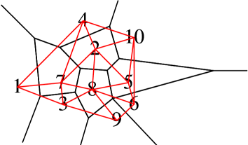
Figure 1: Left: the Voronoi diagram (black lines) of ten points in a plane, numbered 1…10. Superimposed, in red, is the Delaunay triangulation. Right: CPU time taken to cluster $N$ particles for various jet-finders. FastJet is available at http://www.lpthe.jussieu.fr/~salam/fastjet.

The FastJet algorithm has been implemented in the C++ code FastJet. The building and the updating of the Voronoi diagram have been performed using the publicly available Computational Geometry Algorithms Library (CGAL) $\!{}^{{\bf?}}$, in particular its triangulation components $\!{}^{{\bf?}}$. The resulting running time for the clustering of $N$ particles is displayed in fig. 1. It can be seen to be faster than all other codes currently used, both of cone or $k_{t}$ type. Analyses of events with extremely high multiplicity, like heavy ion collisions at the LHC, are now feasible, their clustering taking only about 1 second, rather than 1 day of CPU time.

The speed of FastJet does more, however, than just making analyses with a few hundred particles faster, or those with a few thousand possible. In fact, it allows one to do new things. One example is the possibility of calculating the area of each jet by adding to the event a large number of extremely soft ‘ghost’ particles, and counting how many get clustered into any given jet. This approach is of course computationally heavy, and would be unfeasible – or at least extremely impractical – with a slower jet-finder. Fig. 2 shows the result of this procedure on a LHC event made of one hard and many soft jets. Estimating jet areas is of course not interesting by itself, but as an intermediate step towards performing an event-by-event subtraction of underlying event/minimum bias energy from the hard jets. This work is presently in progress $\!{}^{{\bf?}}$.

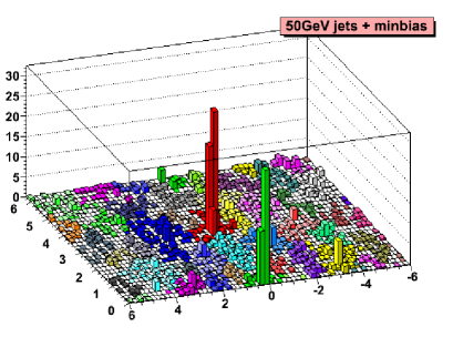
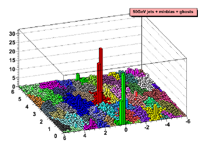
Figure 2: A simulated “typical” event at high luminosity at the LHC. Left: A single event with two hard jets has been combined with about 10 softer events. Right: Very soft ‘ghost’ particles have been added in order to be able to quantify more precisely the area of each jet.

Acknowledgements. I wish to thank Gavin Salam for the ongoing entertaining collaboration on this project.

References

- [1] G. Sterman and S. Weinberg, Phys. Rev. Lett. 39 (1977) 1436.
- [2] See e.g. F. Abe et al. [CDF Collaboration], Phys. Rev. D 45, 1448 (1992); G. C. Blazey et al., hep-ex/0005012.
- [3] S. Catani, Y. L. Dokshitzer, M. Olsson, G. Turnock and B. R. Webber, Phys. Lett. B 269, 432 (1991); S. Catani, Y. L. Dokshitzer, M. H. Seymour and B. R. Webber, Nucl. Phys. B 406, 187 (1993); S. D. Ellis and D. E. Soper, Phys. Rev. D 48, 3160 (1993) [hep-ph/9305266].
- [4] M. H. Seymour, Z. Phys. C 62, 127 (1994).
- [5] M. H. Seymour, hep-ph/0007051.
- [6] R. B. Appleby and M. H. Seymour, JHEP 0212, 063 (2002) [hep-ph/0211426]; A. Banfi and M. Dasgupta, Phys. Lett. B 628, 49 (2005) [hep-ph/0508159].
- [7] J. M. Butterworth, B. E. Cox and J. R. Forshaw, Phys. Rev. D 65, 096014 (2002) [hep-ph/0201098].
- [8] M. Cacciari and G. P. Salam, arXiv:hep-ph/0512210.
- [9] G. L. Dirichlet, J. Reine und Ang. Math. 40 (1850) 209; G. Voronoi, J. Reine und Ang. Math. 133 (1908) 97; See also: F. Aurenhammer, ACM Comp. Surveys 23 (1991) 345; A. Okabe, B. Boots, K. Sugihara and S. N. Chiu (2000). Spatial Tessellations — Concepts and Applications of Voronoi Diagrams. 2nd edition. John Wiley, 2000.
- [10] S. Fortune, in Proceedings of the second annual symposium on Computational geometry, p. 312 (1986).
- [11] O. Devillers, S. Meiser, M. Teillaud, Comp. Geom.: Theory and Applications 2, 55 (1992); O. Devillers, cs.CG/9907023
- [12] A. Fabri et al., Softw. Pract. Exper. 30 (2000) 1167
- [13] J.-D. Boissonnat et al., Comp. Geom. 22 (2001) 5.
- [14] M. Cacciari and G.P. Salam, work in progress