CLOSING TALK: QCD MORIOND 2006

I comment on some of the theoretical work presented at QCD Moriond, 2006

One of the advantages of giving the closing talk at a conference with only plenary sessions, is that a summary is certainly superfluous. I shall take full advantage of that freedom in my talk and present only a few topics.

1 QCD at High Energy

Figure 1: Total deep inelastic scattering cross section vs. $\tau$ [1].

In the infinite momentum frame (IMF) a proton or nucleus is seen as a Lorentz contracted disk, and $xg(x,Q^{2})$ is the number of gluons per unit rapidity of transverse size less than $1/Q$ on that disk. At small $x$ the number of gluons becomes so large that there is a saturation in the growth of the number of gluons. As a consequence of this saturation, the total virtual-photon proton scattering cross section satisfies a geometrical scaling law $\!{}^{{\bf?}}$ as shown in Fig. 1,

$$\sigma(x,Q^{2})\to\sigma(\tau),\;\;\tau=Q^{2}/Q_{s}^{2}(x),\;\;Q_{s}(x)=(x/x_{0})^{\lambda},\;\;\lambda=0.3\;\;.$$ (1)

$Q_{s}(x)$ is the $x$-dependent saturation scale.

1.1 Recent developments

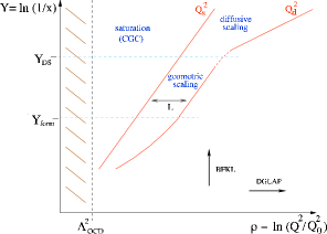
Figure 2: A modern view of the phase diagram of QCD [2].

Recent work in this area is beginning to look in more detail at the region near and beyond the saturation boundary. $\!{}^{{\bf?},{\bf?}}$ While there is geometrical scaling in the region close to the saturation boundary, there are expectations that as one proceeds to small $x$ along the saturation boundary one should arrive at a region of diffusive scaling

$$\sigma(x,Q^{2})\to\sigma\Big{(}\frac{\ln\tau}{\sqrt{Y}}\Big{)},\;\;Y=\ln(1/x).$$ (2)

Fig. 2 gives a modern view of the phase diagram of QCD at small $x$. The interest in the region beyond the saturation boundary, (the region of the colour glass condensate), stems from the fact that it is a region of large occupation number, but of weak coupling. Hence it is amenable to perturbative treatment.

2 DIS scattering in the rest frame

The description of deep inelastic scattering (DIS) in the rest frame of the target hadron has been understood for many years. $\!{}^{{\bf?},{\bf?}}$ In this frame the average lifetime of the fluctuation of a virtual photon into a $q\bar{q}$-pair is $\Delta t\sim 1/\Delta E\sim 1/(Mx_{B})$. Thus at small Bjorken $x_{B}$, the virtual photon materializes into a $q\bar{q}$ pair upstream of the target and arrives at the face of nucleon or nucleus in hadronic guise. The dipoles which interact are either small with symmetric longitudinal momenta or large with asymmetric longitudinal momenta, so that the cross-section falls like $1/Q^{2}$ as required by Bjorken scaling.

2.1 Dipole scattering formula

Thus in the target rest frame the high-energy cross section is the product of the wave function of the virtual photon to produce a dipole times the cross section for the dipole to interact. The cross section for the scattering of a longitudinal or transverse photon is

$$\sigma_{L/T}(x,Q^{2})=\int dz\;d^{2}{\bf r}|\Psi_{L/T}(z,r)|^{2}\hat{\sigma}(x,r)\;,$$ (3)

where the dipole cross section is related to the unintegrated gluon distribution function of the IMF description, ${\cal F}(x,{\bf k})$,

$$\hat{\sigma}(x,r)=\frac{4\pi\alpha_{S}}{3}\int\frac{d^{2}{\bf k}}{{\bf k}^{4}}\;{\cal F}(x,{\bf k})\big{(}1-\exp(i{\bf k}\cdot{\bf r})\big{)}\;.$$ (4)

The phenemenological Golec-Biernat-Wusthoff model $\!{}^{{\bf?}}$ attempts to describe the dipole cross section for all $r$. At small $r$, the cross section $\sigma\sim r^{2}$, which is the mathematical expression of the phenomenon of colour transparency. At large $r$, the dipole cross section is bounded by an energy independent value $\sigma_{0}$ which assures the unitarity of $F_{2}$,

$$\hat{\sigma}(r,x)\,=\,\sigma_{0}\,\left\{1-\exp\left(-\frac{Q_{s}^{2}(x)r^{2}}{4}\right)\right\}\;.$$ (5)

The transition between the two regimes is controlled by the saturation scale $Q_{s}(x)$, which increases with increasing $1/x$. The GBW model can be improved by several refinements, such as the inclusion of impact parameter dependence and the incorporation of perturbative evolution in the dipole cross section. $\!{}^{{\bf?}}$ In addition, heavy flavours can be included in the wave function of the virtual photon. $\!{}^{{\bf?}}$

The advantage of this approach is that the model of a dipole interacting with a nucleus at rest also gives information about the structure of jets and rapidity gaps in the event. This in turn can be used to make predictions for diffraction, shadowing, and vector meson production. Thus we see that the formulation of DIS in the rest frame gives an appealing physical picture, which has predictivity beyond inclusive scattering. Although, in the end, all physics must be Lorentz invariant, the description is less clear in the infinite momentum frame.

2.2 Diffraction in hadron-hadron scattering

The models for diffraction in hadron-hadron scattering have not yet been refined and informed by data to the extent achieved in DIS. In an interesting report the CDF collaboration has reported 3 diphoton candidates in diffractive events. $\!{}^{{\bf?}}$ Although the background to this data has not yet been estimated, such measurements certainly have the potential to help in the estimation of diffractive production of other particles, such as the Higgs boson. The issue of the diffractive Higgs cross section and hard scattering corrections certainly needs to be resolved. $\!{}^{{\bf?}}$ Current estimates of the cross sections for the production of standard model Higgs bosons tend to be rather low. As described by De Roeck and Khoze $\!{}^{{\bf?},{\bf?}}$ the exclusive diffractive Higgs production cross section, $pp\to pHp$ is estimated to be 3-10 fb,whereas the inclusive Higgs production cross section, $pp\to pXHYp$ is 50-200fb. Thus for a standard model Higgs one expects 11(10) signal(background) events for Higgs production in 30 fb^-1.

3 Spin and $\Delta g$

The total spin of the proton is made up the contributions of quarks, gluons and their angular momentum, $\frac{1}{2}=\frac{1}{2}\eta_{\Sigma}+\eta_{g}+<L_{z}>$, where $\eta_{g}=\int dx(g^{\uparrow}-g^{\downarrow})$ etc. As described by Yuan $\!{}^{{\bf?}}$, the historical results, $\eta_{\Sigma}=\eta_{u}+\eta_{d}+\eta_{s}=0.3\pm 0.1$ and $\eta_{s}=-0.1\pm 0.03$ are at variance with naive quark model ideas, and have stimulated a number of experiments to measure the spin carried by the gluons directly. The possibility that the spin carried by the gluon might be large is motivated by the evolution equations for the first moments of the spin-dependent structure functions,

$$\frac{d}{d\ln Q^{2}}\;\eta_{\Sigma}(t)=0+O(\alpha_{s}^{2}),\;\;\frac{d}{d\ln Q^{2}}\;\alpha_{S}(t)\eta_{g}(t)=0+O(\alpha_{s}^{2})\;,$$ (6)

which indicate that $\alpha_{s}\times$gluon contribution is formally of the same order as the quark contribution. Early experiments will not be able to make very precise statements about $\eta_{g}$, but they should be able to indicate whether a sizeable fraction of the total spin of one half is carried by the gluons, and a fortiori, whether the spin carried by the gluons is so large,

$$\eta_{g}(4~{}{\rm GeV}^{2})=2,\;\;(\eta_{s}\sim-\frac{\alpha_{S}}{2\pi}\eta_{g})\;,$$ (7)

that it can explain the apparent discrepancy with naive quark model ideas.

At this meeting there were new experimental results $\!{}^{{\bf?},{\bf?},{\bf?}}$ sensitive to $\eta_{g}$, but the overall picture is unchanged. The experimental results give little comfort to the idea that $\eta_{g}$ could be as large as 2, although because current experiments only have limited/smeared coverage in $x$, it is hard to make more exact statements. In my opinion a definitive measurement of the polarized gluon will only come using a process which has been successfully used to determine the unpolarized gluon. In all likelihood this will require measurement of direct photon production in polarized scattering at RHIC.

4 B-physics

Fig. 3 shows the remarkable progress in the knowledge of the Unitarity triangle since the advent of the $B$-factories. The 1995 plot $\!{}^{{\bf?}}$ contains only the three quantities, $V_{ub},\epsilon_{K}$ and $\Delta m_{B_{d}}$ and region 1a corresponds to a scan over a $1\sigma$ ranges of the input parameters. The 2006 plot $\!{}^{{\bf?}}$ includes the information on $\Delta m_{s}$ coming from the Tevatron.

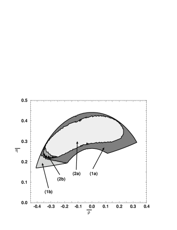
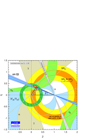
Figure 3: The constraints on the unitarity triangle in 1995 (left) and in Winter 2006, [16,17].

4.1 B-physics at the Tevatron

The potential of hadron machines to do B-physics stems from the large cross section, and from the fact that all types of B-mesons and B-baryons are produced. At the Tevatron, usable $B$’s are produced at a rate of about 50 Hz. New results on $B_{s}$ mixing indicate that the Tevatron is beginning to live up to that potential. From the D0 study of $B_{s}$-mixing $\!{}^{{\bf?},{\bf?}}$, the log likelihood curve has a preferred value at the oscillation frequency $\Delta m_{s}=19~{}$ps^-1 with a 90% confidence level interval $17<\Delta m_{s}<21~{}$ps^-1. D0 are therefore close to an interesting $B_{s}$ mixing measurement. After the conference was over, CDF $\!{}^{{\bf?}}$ announced a measurement of $\Delta m_{s}$

$$\Delta m_{s}=17.31^{+0.33}_{-0.18}(stat)\pm 0.07(sys)~{}\mbox{ps}^{-1}.$$ (8)

On the basis of this measurement CDF deduce that $\frac{|V_{td}|}{|V_{ts}|}=0.208^{+0.001}_{-0.002}\mbox{(stat +sys)}^{+0.008}_{-0.006}\mbox{(theory)}$.

I shall now discuss the source of the theoretical error in this measurement. Mixing in the neutral $B$ system is determined by box diagrams, leading to the formula

$$\Delta m_{B_{q}}\sim f_{B_{q}}^{2}\,B_{B_{q}}\,m_{B_{q}}\,|V_{tb}^{*}V_{tq}|^{2}$$ (9)

Within the CKM model, $B_{s}$ mixing is used primarily to control hadronic uncertainties, which are present in the decay constant, $f_{B_{q}}$ and the bag parameter $B_{B_{q}}$. We shall see that even with the cancellations inherent in taking the ratio $\Delta m_{B_{d}}/\Delta m_{B_{s}}$ the level at which the hadronic parameters are currently controlled by lattice gauge theory is now inadequate.

4.2 Lattice results for decay constants, $f_{B}$ and bag parameters, $B$

The results from unquenched lattice results QCD are $\!{}^{{\bf?}}$,

$$f_{B}=216(09)(19)(07)~{}{\rm MeV},\;\;f_{B_{s}}=249(07)(26)(09)~{}{\rm MeV}\;.$$ (10)

The largest error is due to the fact that matching for the weak current operator between the continuum and the lattice is performed at one loop. However the matching error (and some other errors) cancel in the ratio, leading to a 4% prediction.

$$\frac{f_{B_{s}}}{f_{B_{d}}}=1.20(3)(1)\;.$$ (11)

The bag parameter is determined by the JLQCD collaboration to be $\!{}^{{\bf?}}$

$$B_{B_{d}}(m_{b})=0.836(27)^{(+56)}_{(-62)},\;\;\frac{B_{B_{d}}}{B_{B_{d}}}=1.017(16)^{(+56)}_{(-17)}\;.$$ (12)

This gives us an 11% prediction $f_{B_{d}}\sqrt{B_{B_{d}}}=244(26){\rm MeV}$, but a 4% prediction for the ratio $\frac{f_{B_{s}}\sqrt{B_{B_{s}}}}{f_{B_{d}}\sqrt{B_{B_{d}}}}=1.210^{+47}_{-35}$. In summary the ratio $\xi=\frac{f_{B_{d}}\sqrt{B_{B_{d}}}}{f_{B_{s}}\sqrt{B_{B_{s}}}}$ is calculated by lattice gauge theory $\!{}^{{\bf?}}$,

$$\xi=\frac{\Phi(B_{s})}{\Phi(B_{d})}=1.210^{+0.047}_{-0.035}.$$ (13)

Fig. 4, taken from ref. [23], shows the importance of the low mass points in determining the chiral extrapolation to the physical mass, shown by the vertical dashed line.

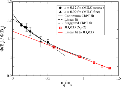
Figure 4: Extrapolation of lattice results to the physical mass using JLQCD and HPQCD data [23].

Using this value for the ratio we can extract $|V_{td}/V_{ts}|$ using eq. (9),

$$\Big{|}\frac{V_{td}}{V_{ts}}\Big{|}=\lambda\sqrt{(1-\bar{\rho})^{2}+\bar{\eta}^{2}}=\sqrt{\frac{\Delta m_{B_{d}}}{\Delta m_{B_{s}}}}\;\sqrt{\frac{m_{B_{s}}}{m_{B_{d}}}}\;\frac{f_{B_{s}}\sqrt{B_{B_{s}}}}{f_{B_{d}}\sqrt{B_{B_{d}}}}\;.$$ (14)

The 4% error on $\xi$ has now become the limiting uncertainty, about four times larger than the error on $\sqrt{\frac{\Delta m_{B_{d}}}{\Delta m_{B_{s}}}}$.

5 QCD engineering and the challenge of the LHC

In order to assess the challenge presented by the LHC data, I shall consider the physics of top production. Since some of the motivation for the LHC is to discover objects with large masses, top production is an interesting paradigm for future studies. Examples of lowest order diagrams for the pair production of top and for single top production are shown in Fig. 5.

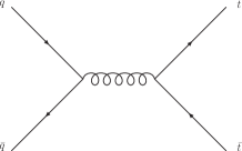
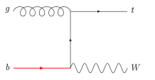
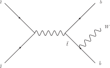
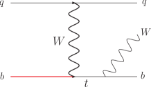
Figure 5: Lowest order diagrams for pair- and single-top production

Process	Tevatron[pb]	LHC[pb]
$t\bar{t}$	6	720
$t\bar{b}$	0.8	10
$tq$	1.8	240
$Wt$	0.14	66

Table 1: Top production cross sections at $\sqrt{s}=1.96$ TeV.

Table 1 gives the total next-to-leading order (NLO) cross-sections for $t\bar{t}$ production both at the Tevatron and the LHC. $\!{}^{{\bf?},{\bf?}}$ The total single top cross-section is smaller than the $t{\bar{t}}$ rate by about a factor of two, at both machines. However, despite the sizeable cross section, single top production has not yet been observed at the Tevatron. This is undoubtedly due to the large number of backgrounds shown in Fig. 6.

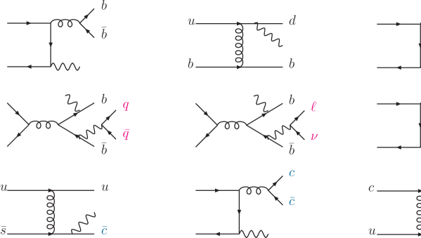
Figure 6: Backgrounds for single top production

Process	$\sigma$ [fb]
$q\bar{q}\to W+b+\bar{b}$	30
$q\bar{q}\to W+g+g$	35
$us\to W+u+c$	19
$ub\to W+d+b$	11
$q\bar{q}\to W+c+\bar{c}$	6
$uc\to W+d+c$	3
$q\bar{q}\to W+Z(b\bar{b})$	3
$q\bar{q}\to t\bar{t}\to Wb\bar{b}q\bar{q}$	6
$q\bar{q}\to t\bar{t}\to Wb\bar{b}l\nu$	3

Table 2: Cross-sections in fb include nominal tagging efficiences and mis-tagging/fake rates

The background processes shown in Fig. 6 are calculated with MCFM at $\sqrt{s}=1.96$ TeV and the results are given given in Table 2. For the cuts and efficiencies used we refer the reader to Tables VI,VIII of ref. [25]. With the same set of cuts, the signal rates are $7$ fb and $11$ fb for $s$- and $t-$channel respectively. Thus, with our nominal efficiencies, the ratio of signal:background is only $1:6$.

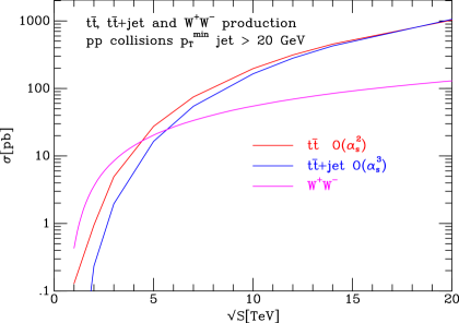
Figure 7: Cross section for $t\bar{t}$, $t\bar{t}+\mbox{jet}$ and $W^{+}W^{-}$ production as a function of energy

Another feature of top production which merits consideration is the production of jets in association with top quarks. Fig. 7 shows that for a jet with $p_{T}^{min}>20$ GeV, $\sigma(t\bar{t}+{\rm jet})>\sigma(t\bar{t})$ at the energy of the LHC. Radiation of one gluon in general will not be enough and the parton shower needs to be included.

These examples make it clear that there is a large amount of work needed to understand LHC data. Just as in the single top case, signal processes will be accompanied by many backgrounds. In the best of all worlds these backgrounds will be measured directly in the experiments, but in the case of irreducible backgrounds, one will have to rely on theoretical calculations.

The approaches to calculating Feynman amplitudes have been nicely reviewed by Del Duca. $\!{}^{{\bf?}}$ The various techniques which have been used are tree graphs, tree graphs combined with showers, NLO calculations, NLO calculations combined with showers, and NNLO calculations. Specializing for the moment to NLO, Fig. 8 illustrates the point that the state of the art can calculate loops or legs, but not both.

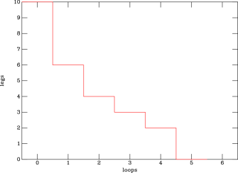
Figure 8: Schematic description of the state of the art in multileg calculations

At LHC processes with many legs will be produced. Phenemonologically interesting processes involve vector bosons, leptons, missing energy, heavy flavours. Just as in the top case, many processes can contribute to the same signature, which argues for a unified approach to NLO calculations.

The computer program MCFM $\!{}^{{\bf?}}$, which is a general purpose NLO code, is an attempt to provide such a tool.

$p{\bar{p}}\to W^{\pm}/Z$	$p{\bar{p}}\to W^{+}+W^{-}$
$p{\bar{p}}\to W^{\pm}+Z$	$p{\bar{p}}\to Z+Z$
$p{\bar{p}}\to W^{\pm}+\gamma$	$p{\bar{p}}\to W^{\pm}/Z+H$
$p{\bar{p}}\to W^{\pm}+g^{\star}\,(\to b{\bar{b}})$	$p{\bar{p}}\to Zb{\bar{b}}$
$p{\bar{p}}\to W^{\pm}/Z+\mbox{1 jet}$	$p{\bar{p}}\to W^{\pm}/Z+\mbox{2 jets}$
$p{\bar{p}}(gg)\to H$	$p{\bar{p}}(gg)\to H+\mbox{1 jet}$
$p{\bar{p}}(VV)\to H+\mbox{2 jets}$	$p{\bar{p}}\to t+q$
$p{\bar{p}}\to H+b$	$p{\bar{p}}\to Z+b$

Table 3: Processes available in MCFM

Knowledge of these processes at NLO provides the first precise predictions of their event rates. MCFM and other similar programs are a start, but they are clearly insufficient for the needs at the LHC. The stumbling block which prevents the inclusion of further processes is the calculation of one-loop corrections.

6 Techniques for one loop diagrams

One of the early general calculations of one loop corrections was performed by Passarino and Veltman. $\!{}^{{\bf?}}$ More recent general purpose attempts have used semi-numerical results, which reduce an arbitrary diagram using numerical methods to a sum of scalar integrals, which are known analytically. Recent results in this field are the one-loop matrix element for a Higgs plus four partons and the six-gluon amplitudes. $\!{}^{{\bf?}}$

6.1 Analytical techniques

In addition to the semi-numerical techniques great progress has been made in the analytical calculation of loop amplitudes. In this field the key ideas are supersymmetric decomposition, MHV diagrams, BCFW recursion, unitarity and unitarity using multiple cuts. Although this is a field which is developing rapidly, recent reviews are given in refs. [30,31].

6.2 Outlook: analytic vs numerical

The new analytical methods lead to beautiful results for gauge theory tree graph amplitudes. However the evaluation of tree graphs is already solved numerically by Berends-Giele recursion. $\!{}^{{\bf?}}$ For tree graphs the issue reduces merely to a question of numerical expediency which has been addressed in ref. [33]. So far the impact on real phenomenology is rather limited, although simple tree graph results have been obtained for Higgs+5 parton amplitudes. $\!{}^{{\bf?},{\bf?}}$

The extension of these techniques to loops in QCD is the next frontier. The new techniques solve the problem of computing one-loop amplitudes of gluons in ${\cal N}=4$ super Yang-Mills. So far only partial analytic results for $n\geq 6$ QCD amplitudes have been published. However there is great intellectual excitement and an injection of personnel from formal areas. There is no doubt that analytic results, when available, are superior to numerical, or seminumerical methods. It is primarily a question of expediency. Which technique will lead first to useful NLO results for the many multi-leg processes which we are interested in at the LHC?

7 Beyond NLO?

7.1 NLO and parton showers

A remarkable theoretical advance of the last few years has been the consistent combination of NLO calculations with parton shower Monte Carlo programs. The output is a set of events, which are fully inclusive. Total rates are accurate to NLO in the sense that NLO results are recovered for all observables upon expansion in $\alpha_{S}$. Currently a limited number of available processes, single vector boson production, $W/Z/H$, vector boson pair production, $WW$, heavy quark pair, $Q\bar{Q}$ $\!{}^{{\bf?}}$, and single top production. $\!{}^{{\bf?}}$ It is clear that MC@NLO relies on the appropriate NLO process having been calculated.

As an example I show a curve obtained for $t\bar{t}$-production using MC@NLO. Figure 9 shows the prediction of forward-backward asymmetry at the Tevatron. $\!{}^{{\bf?}}$ The asymmetry is generated beyond the leading order in perturbation theory $\!{}^{{\bf?}}$ and is well reproduced by MC@NLO.

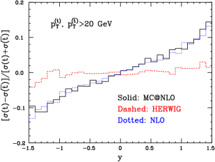
Figure 9: Asymmetry in top production at the Tevatron, [36].

7.2 What quantities do we want to calculate at NNLO?

The quantities we need to calculate are those quantities which are will be measured at high precision. It is especially important to calculate fully differential results, to correctly account for experimental cuts. A partial list includes,

• $e^{+}e^{-}\to 3$ jets, ($\alpha_{S}$)

• Fully exclusive $pp\to W,Z,\gamma^{*}$, (parton luminosity)

• $pp\to 2$ jets (gluon distribution function)

• $pp\to\gamma$+jet (jet energy scale).

Petriello presented a new result on $W$ production at NNLO including the spin correlations. $\!{}^{{\bf?}}$ For the electron $p_{T}>M_{W}/2$ one has effectively a NLO process; corrections of order 20% are found. In other regions, a perturbation theory uncertainty at the per cent level is found.

8 Conclusions

This week has given testimony to the experimental and theoretical vibrancy of QCD. Building on persuasive description of Deep Inelastic data from HERA in the QCD improved dipole model theorists have been exploring the structure of the nucleon and the nucleus at high energy beyond the saturation limit. The start of the era of precision $B$ physics at hadronic colliders, and, in particular, the measurement of $B_{s}$ mixing, presents new challenges for the calculation of hadronic parameters from lattice gauge theories.

Lastly, the interpretation of data from LHC will require puts new demands on QCD calculations, at leading order, next-to-leading order (NLO), NLO+parton shower and even at next-to-next-to-leading order. It will also require an extensive program of validation of these calculations against data and against themselves. The LHC begins in about a year, so for the experimenters, the era of giving talks about ’Studies at the LHC’ without the benefit of data is almost over. The exploration of a completely new range of energy is a once-in-a-lifetime opportunity for most of us. Looking further ahead, the continued exploration of the energy frontier beyond the LHC, requires the success of the LHC experiments.

References

References

- [1] A. M. Stasto, K. Golec-Biernat and J. Kwiecinski, Phys. Rev. Lett. 86, 596 (2001) [arXiv:hep-ph/0007192].
-
[2]
E. Iancu, these proceedings,
E. Iancu, C. Marquet and G. Soyez, arXiv:hep-ph/0605174. - [3] M. Lublinsky, these proceedings, arXiv:hep-ph/0605025.
- [4] K. Golec-Biernat and M. Wusthoff, Phys. Rev. D 59, 014017 (1999) [arXiv:hep-ph/9807513].
- [5] V. Gribov, Sov. Phys. JETP 30 (1969) 709.
-
[6]
J.D. Bjorken, in Proc. of the International Symposium on
Electron and Photon Interactions at High Energies, (Cornell, 1971) 281;
J.D. Bjorken and J.B. Kogut, Phys. Rev. D8 (1973) 1341. - [7] H. Kowalski, these proceedings.
- [8] S. Sapeta, arXiv:hep-ph/0605154.
- [9] K. Terashi [CDF Collaboration], these proceedings, arXiv:hep-ex/0605084.
- [10] A. de Roeck, these proceedings.
- [11] V. Khoze, these proceedings.
- [12] F. Yuan, these proceedings.
- [13] R. Fatemi, these proceedings, arXiv:nucl-ex/0606007.
- [14] S. Procureur, these proceedings, arXiv:hep-ex/0605043.
- [15] K. O. Eyser [PHENIX Collaboration], these proceedings, arXiv:nucl-ex/0605023.
- [16] S. Herrlich and U. Nierste, Phys. Rev. D 52, 6505 (1995) [arXiv:hep-ph/9507262].
- [17] CKMfitter Group (J. Charles et al.), Eur. Phys. J. C41, 1-131 (2005) [hep-ph/0406184], updated results and plots available at: http://ckmfitter.in2p3.fr
- [18] D0, D0note 5045-CONF.
- [19] M. Naimuddin, these proceedings, arXiv:hep-ex/0605057.
- [20] CDF, hep-ex/0606027.
- [21] A. Gray et al. [HPQCD Collaboration], Phys. Rev. Lett. 95, 212001 (2005) [arXiv:hep-lat/0507015].
- [22] S. Aoki et al. [JLQCD Collaboration], Phys. Rev. Lett. 91, 212001 (2003) [arXiv:hep-ph/0307039].
- [23] M. Okamoto, PoS LAT2005, 013 (2006) [arXiv:hep-lat/0510113].
- [24] J. Campbell, R. K. Ellis and F. Tramontano, Phys. Rev. D 70, 094012 (2004) [arXiv:hep-ph/0408158].
- [25] J. Campbell and F. Tramontano, Nucl. Phys. B 726, 109 (2005) [arXiv:hep-ph/0506289].
- [26] V. Del Duca, these proceedings, arXiv:hep-ph/0606263.
- [27] R.K. Ellis and J.M. Campbell, http://mcfm.fnal.gov
- [28] G. Passarino and M. J. G. Veltman, Nucl. Phys. B 160, 151 (1979).
- [29] G. Zanderighi, these proceedings, arXiv:hep-ph/0605175.
- [30] F. Cachazo and P. Svrcek, PoS RTN2005, 004 (2005) [arXiv:hep-th/0504194].
- [31] L. J. Dixon, PoS HEP2005, 405 (2006) [arXiv:hep-ph/0512111].
- [32] F. A. Berends and W. T. Giele, Nucl. Phys. B 306, 759 (1988).
- [33] M. Dinsdale, M. Ternick and S. Weinzierl, JHEP 0603, 056 (2006) [arXiv:hep-ph/0602204].
- [34] S. D. Badger, E. W. N. Glover and V. V. Khoze, JHEP 0503, 023 (2005) [arXiv:hep-th/0412275].
- [35] L. J. Dixon, E. W. N. Glover and V. V. Khoze, JHEP 0412, 015 (2004) [arXiv:hep-th/0411092].
- [36] S. Frixione, P. Nason and B. R. Webber, JHEP 0308, 007 (2003) [arXiv:hep-ph/0305252].
- [37] S. Frixione, E. Laenen, P. Motylinski and B. R. Webber, JHEP 0603, 092 (2006) [arXiv:hep-ph/0512250].
- [38] P. Nason, S. Dawson and R. K. Ellis, Nucl. Phys. B 303, 607 (1988).
-
[39]
F. Petriello, these proceedings,
K. Melnikov and F. Petriello, arXiv:hep-ph/0603182.