Lifetimes of the Heavy Neutral Leptons in the Okamura Model

Abstract

We study the lifetimes of TeV-scale heavy neutral leptons (Majorana neutrinos) that appear in a model suggested by Okamura et al. okamura . We develop a convenient way to parametrize the neutrino mass texture of the model, and illustrate our method by calculating the mass spectrum, decay widths, and lifetimes of the heavy particles over the entire parameter space. From the mass spectrum, we find that for most of the parameter space, only two-body decays are relevant in the calculation of the lifetime, with typical values falling in the range of $10^{-26}$ to $10^{-24}$ seconds. If the particles discussed here are created at colliders, their lifetimes are short enough for them to decay inside the detector, while long enough to lead to a narrow peak in the invariant mass spectrum of the decay products. However, an analysis by Dicus, Karatas, and Roy Dicus:1991fk suggests that they may be difficult to observe at the LHC.

I Introduction.

Several models of neutrino mass have been suggested in the literature in which the neutrinos acquire masses through a seesaw seesaw type mass texture, but the Majorana masses of the right-handed neutrinos are at the TeV scale instead of the GUT scale of $\sim 10^{16}$ GeV okamura ; Chang:1994hz ; Carone:1996ny ; Arkani-Hamed:2000bq ; Ma:2000cc . The smallness of the neutrino masses in those models is achieved either by the reduction of the rank of the mass matrix through a judicious choice of mass texture okamura ; Chang:1994hz , or by the suppression of the Dirac masses through an extended Higgs sector Carone:1996ny ; Arkani-Hamed:2000bq ; Ma:2000cc .

In such models, the heavy, mostly-right-handed mass eigenstates typically have masses of a few TeV, placing them within reach of the CERN Large Hadron Collider (LHC) or future $e^{+}e^{-}$ linear colliders. If created, the particles will decay into a light neutrino+Higgs through the Yukawa interaction responsible for the Dirac masses, or into a light neutrino+$Z$ or a charged lepton+$W$ through the small admixture of the left-handed neutrino state. This last decay mode is particularly interesting since the decay products can be all visible. Of course, whether such a decay, and thus the particle, can be observed at colliders or not depends on whether the lifetime of the particle is short enough for it to decay inside the detector, and if that is the case, whether the width is small enough so that a narrow peak is discernible in the invariant mass of its decay products.

In this paper, we calculate the lifetimes of the heavy, mostly-right-handed states of the model proposed by Okamura et al. in Ref. okamura . The original motivation of the model was to explain the NuTeV anomaly Zeller:2001hh ; Davidson:2001ji , one possible solution of which requires largish mixing ($\theta^{2}\sim 0.003$) between the light and heavy ($\gg M_{Z}$) neutrino states nutev . Denoting the left- and right-handed neutrino states by $\nu$ and $\xi$, respectively, the Okamura texture is given by

$$\left[\;\overline{\nu^{c}_{1}}\;\;\overline{\nu^{c}_{2}}\;\;\overline{\nu^{c}_{3}}\;\;\overline{\xi}_{1}\;\;\overline{\xi}_{2}\;\;\overline{\xi}_{3}\;\right]\left[\begin{array}[]{cccccc}0&0&0&\alpha m&\beta m&\gamma m\\ 0&0&0&\alpha m&\beta m&\gamma m\\ 0&0&0&\alpha m&\beta m&\gamma m\\ \alpha m&\alpha m&\alpha m&\alpha M&0&0\\ \beta m&\beta m&\beta m&0&\beta M&0\\ \gamma m&\gamma m&\gamma m&0&0&\gamma M\\ \end{array}\right]\left[\begin{array}[]{c}\nu_{1}\\ \nu_{2}\\ \nu_{3}\\ \xi^{c}_{1}\\ \xi^{c}_{2}\\ \xi^{c}_{3}\end{array}\right]\;,$$ (1)

where the dimensionless parameters $\alpha$, $\beta$, and $\gamma$ are in general complex and assumed to satisfy the relation

$$\alpha+\beta+\gamma=0\;.$$ (2)

This condition reduces the rank of the above mass matrix to three, leading automatically to three massless neutrino states. Though the actual light, mostly left-handed neutrino states in nature are not completely massless, this model suffices as a first approximation. We fix the normalization of the three complex parameters $\alpha$, $\beta$, and $\gamma$ to

$$|\alpha|^{2}+|\beta|^{2}+|\gamma|^{2}=3\;.$$ (3)

The dimensionful parameters $m$ and $M$ can be taken to be real and they set the scale of the Dirac and Majorana masses, respectively. The solution to the NuTeV anomaly requires their ratio to be nutev ; okamura

$$\frac{m}{M}\sim 0.03\;.$$ (4)

If the gauge singlet states $\xi_{i}$ $(i=1,2,3)$ couple to other particles only through the Yukawa interactions which generate the Dirac submatrix of Eq. (1), then any permutation of the three complex parameters $\alpha$, $\beta$ and $\gamma$ leads to the exact same model since we will have the freedom to relabel the three gauge singlet states without affecting any physics. In those cases, there exist a $3!=6$ fold redundancy in the parameter space spanned by $\alpha$, $\beta$, and $\gamma$. This will be assumed in the following.

If we set $M=0$ in Eq. (1), we obtain

$$\left[\begin{array}[]{cccccc}0&0&0&\alpha m&\beta m&\gamma m\\ 0&0&0&\alpha m&\beta m&\gamma m\\ 0&0&0&\alpha m&\beta m&\gamma m\\ \alpha m&\alpha m&\alpha m&0&0&0\\ \beta m&\beta m&\beta m&0&0&0\\ \gamma m&\gamma m&\gamma m&0&0&0\end{array}\right]\;$$ (5)

which is manifestly rank 2. The non-zero eigenvalues of this matrix are

$$\pm m\sqrt{3\left(|\alpha|^{2}+|\beta|^{2}+|\gamma|^{2}\right)}=\pm 3\,m\;.$$ (6)

Therefore, this mass texture leads to four massless and two massive Majorana fermions. Pairing up the Majorana fermions with the same mass and opposite CP, we can reduce the set to one massive and two massless Dirac fermions bilenky . If we assume that the up-type quarks share the same Dirac mass texture as the neutrinos, as would be the case in the Pati-Salam model Pati:uk , we obtain one massive quark which can be identified with the $t$, and two massless quarks which can be identified with the $u$ and the $c$. To produce the $t$ quark mass, we need

$$m\sim 60\,\mathrm{GeV}\;,$$ (7)

which together with Eq. (4) implies

$$M\sim 2\,\mathrm{TeV}\;.$$ (8)

Fixing $m$ and $M$ to these values, the parameter space of the Okamura model is given by the values of $\alpha$, $\beta$, and $\gamma$ which satisfy Eqs. (2) and (3).

In the following, we introduce a convenient graphical representation of the parameter space for the Okamura model, and calculate the masses and lifetimes of the three heavy mass eigenstates over it. We find that except for the vicinity of three isolated points at the ‘edge’ of the parameter space, the three masses are always in the TeV range, and the lifetimes are typically in the range of $10^{-26}$ to $10^{-24}$ seconds. In terms of the widths, these correspond to the range of $0.7\sim 70$ GeV, which are fairly narrow compared to the masses.

II The Parameter Space of the Okamura Model

Figure 1: The three complex numbers $\alpha$, $\beta$ and $\gamma$ satisfying $\alpha+\beta+\gamma=0$ form a close triangle. For each choice of the three lengths $|\alpha|$, $|\beta|$, and $|\gamma|$, there are two possible orientations of the triangle ($\odot$ and $\otimes$) which are related by complex conjugation (1st and 2nd columns). However, the $\otimes$ case is equivalent to the $\odot$ case with the lengths $|\beta|$ and $|\gamma|$ interchanged (2nd and 3rd columns).

We begin by noting that for the three complex parameters $\alpha$, $\beta$, and $\gamma$ to sum to zero, Eq. (2), they must form a closed triangle when summed tip-to-tail as vectors in the complex plane. Without loss of generality, we can set the phase of $\alpha$ to zero. This can always be achieved by changing the overall phase of $\alpha$, $\beta$ and $\gamma$, and does not affect any physical result. Therefore, the triangle formed by $\alpha$, $\beta$, and $\gamma$ can be assumed to have its base along the positive real axis. We define the “orientation” of this triangle as the direction of the vectorial cross product $\alpha\times\beta$. If the orientation of the triangle is $\odot$ (out of the complex plane), then $\beta$ is in the upper complex plane while $\gamma$ is in the lower complex plane. If the orientation of the triangle is $\otimes$ (into the complex plane), then $\beta$ is in the lower complex plane while $\gamma$ is in the upper complex plane (see Fig. 1). Then, it is easy to see that specifying the lengths of the three sides $|\alpha|$, $|\beta|$, and $|\gamma|$, and the orientation of the triangle is equivalent to specifying the three complex numbers $\alpha$, $\beta$, and $\gamma$.

Furthermore, we need not consider both orientations since the two cases can be transformed into each other by a simple interchange of the lengths of $\beta$ and $\gamma$, and a relabeling of the singlet neutrino fields. As discussed previously, this does not affect any physical result either. Therefore, we will always take the triangle to be in the $\odot$ orientation. This choice also reduces the redundancy of the parameter space from $3!=6$ to 3 since we have used up the freedom to interchange $\beta$ and $\gamma$ to fix the orientation.

This consideration shows that specifying the three lengths $|\alpha|$, $|\beta|$, and $|\gamma|$ suffices to uniquely determine the Okamura texture, with cyclic permutations of the three lengths leading to the same model. (This residual redundancy comes from our freedom to choose which of the three lengths to call $|\alpha|$.) The question then, is, how can we specify those three lengths so they satisfy the normalization condition Eq. (3), and also the triangle inequalities:

$$|\beta|+|\gamma|\geq|\alpha|\;,\quad|\alpha|+|\beta|\geq|\gamma|\;,\quad|\alpha|+|\gamma|\geq|\beta|\;,$$ (9)

so they form a closed triangle? To this end, we utilize the fact that the sum of distances from any point inside a triangle to its three sides is constant: any point inside an equilateral triangle of height three will have distances to the three sides which add up to three. If we identify these distances with $|\alpha|^{2}$, $|\beta|^{2}$, and $|\gamma|^{2}$, we can use the position of the point to specify the three lengths. Requiring the square-roots of these distances to satisfy the triangle inequality constrains the point to be inside a unit circle which inscribes the triangle. Therefore, for every point inside the unit circle, we can associate a corresponding parameter set for the Okamura texture (see Fig. 2).

Figure 2: The distances from any point inside an equilateral triangle of height three to its three sides add up to three. We can use these distances to specify $|\alpha|^{2}$, $|\beta|^{2}$, and $|\gamma|^{2}$. The triangle inequality is satisfied for points inside the unit circle which inscribes the triangle.

If we specify the position of a point inside the unit circle with its polar coordinate $(r,\theta)$, where $0\leq r\leq 1$, $\theta\in[-\pi,\pi)$, the corresponding values of $|\alpha|$, $|\beta|$, and $|\gamma|$ are:

$$|\alpha|=\sqrt{1+r\sin\theta}\;,\quad|\beta|=\sqrt{1+r\sin\left(\theta-\frac{2\pi}{3}\right)}\;,\quad|\gamma|=\sqrt{1+r\sin\left(\theta+\frac{2\pi}{3}\right)}\;.$$ (10)

The phases of the three numbers are:

$$\arg\alpha = \phantom{-}0\;,$$ (11)

$$\arg\beta = \phantom{-}\pi-\cos^{-1}\frac{1/2+r\sin(\theta-\pi/3)}{\sqrt{[\,1+r\sin\theta\,][\,1+r\sin(\theta-2\pi/3)\,]}}\;,$$ (12)

$$\arg\gamma = -\pi+\cos^{-1}\frac{1/2+r\sin(\theta+\pi/3)}{\sqrt{[\,1+r\sin\theta\,][\,1+r\sin(\theta+2\pi/3)\,]}}\;.$$ (13)

In Fig. 3, we plot the dependence of $\arg\beta$ and $\arg\gamma$ on the position of the point inside the unit circle.

A cyclic permutation of $\alpha$, $\beta$, and $\gamma$ which leaves the physics invariant up to an overall phase corresponds to the transformation $\theta\rightarrow\theta+2\pi/3$ ($120^{\circ}$ rotations). This means that we expect the same symmetry to be present in the mass spectrum and the values of heavy neutrino decay widths and lifetimes. This can be used as a useful check of our calculations.

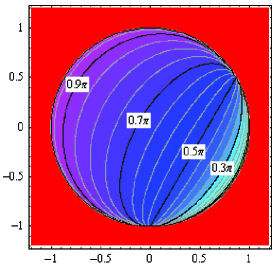
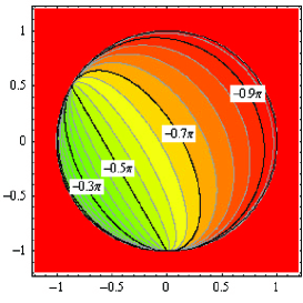
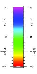
Figure 3: Contour lines and density plots for $\arg\beta$ (left) and $\arg\gamma$ (middle). The distances between two consecutive equipotential lines are $\Delta\arg\beta=\Delta\arg\gamma=0.05\pi$. The color scheme is shown on the right.

III The Lagrangian

To calculate the lifetimes of the heavy neutral states, we must first specify their interactions. We denote the left-handed charged lepton fields with $\ell$, and the left- and right-handed neutrino fields with $\nu$ and $\xi$, respectively:

$$\ell=\left[\begin{array}[]{c}\ell_{1}\\ \ell_{2}\\ \ell_{3}\end{array}\right]\;,\qquad\nu=\left[\begin{array}[]{c}\nu_{1}\\ \nu_{2}\\ \nu_{3}\end{array}\right]\;,\qquad\xi=\left[\begin{array}[]{c}\xi_{1}\\ \xi_{2}\\ \xi_{3}\end{array}\right]\;.$$ (14)

The right-handed neutrino fields, $\xi_{i}$ ($i=1,2,3$), are gauge singlets. The components of the Higgs doublet are denoted

$$H=\left[\begin{array}[]{c}\phi^{+}\\ \phi_{0}\end{array}\right]\;.$$ (17)

Then, the Lagrangian which governs the interaction of the neutrinos is

$$\mathcal{L}=\mathcal{L}_{W,Z}+\mathcal{L}_{H}+\mathcal{L}_{M}\;,$$ (18)

where

$$\mathcal{L}_{W,Z} = \frac{g}{\sqrt{2}}\left(\overline{\ell}\gamma^{\mu}\nu\right)W^{-}_{\mu}+\frac{g}{\sqrt{2}}\left(\overline{\nu}\gamma^{\mu}\ell\right)W^{+}_{\mu}+\frac{g}{2\cos\theta_{W}}\left(\overline{\nu}\gamma^{\mu}\nu\right)Z_{\mu}\;,$$ (19)

$$\mathcal{L}_{H} = -\overline{\xi}\,\lambda\left(\phi^{0}\nu-\phi^{+}\ell\right)+h.c.\;,$$ (20)

$$\mathcal{L}_{M} = -\frac{1}{2}\,\overline{\xi}\,\mathcal{M}\,\xi^{c}+h.c.\;.$$ (21)

We neglect the Yukawa interactions which give rise to the charged lepton masses: the charged leptons are treated as massless as well as the light neutrino states. In the Okamura model, the Yukawa matrix $\lambda$ and the Majorana mass matrix $\mathcal{M}$ are given by

$$\lambda=\frac{\sqrt{2}{m}}{v}\left[\begin{array}[]{ccc}\alpha&\alpha&\alpha\\ \beta&\beta&\beta\\ \gamma&\gamma&\gamma\end{array}\right]\;,\qquad\mathcal{M}=M\left[\begin{array}[]{ccc}\alpha&0&0\\ 0&\beta&0\\ 0&0&\gamma\end{array}\right]\;.$$ (22)

After the neutral Higgs develops a VEV,

$$\left\langle\phi^{0}\right\rangle=\left\langle\phi^{0*}\right\rangle=\frac{v}{\sqrt{2}}\;,$$ (23)

the Yukawa matrix $\lambda$ leads to the Dirac mass matrix of the neutrinos:

$$\mathcal{D}=\frac{v}{\sqrt{2}}\lambda=m\left[\begin{array}[]{ccc}\alpha&\alpha&\alpha\\ \beta&\beta&\beta\\ \gamma&\gamma&\gamma\end{array}\right]\;.$$ (24)

The Goldstone bosons are absorbed into the $W$ and the $Z$, $\phi^{0}\rightarrow 1/\sqrt{2}(h+v)$ as usual, and the resulting Lagrangian is:

$$\mathcal{L} = \frac{g}{\sqrt{2}}\left(\overline{\ell}\gamma^{\mu}\nu\right)W^{-}_{\mu}+\frac{g}{\sqrt{2}}\left(\overline{\nu}\gamma^{\mu}\ell\right)W^{+}_{\mu}+\frac{g}{2\cos\theta_{W}}\left(\overline{\nu}\gamma^{\mu}\nu\right)Z_{\mu}$$ (26)

$$-\overline{\xi}\,\mathcal{D}\,\nu-\frac{1}{\sqrt{2}}\left(\overline{\xi}\,\lambda\,\nu\right)h-\frac{1}{2}\,\overline{\xi}\,\mathcal{M}\,\xi^{c}+h.c.$$

The neutrino mass terms can be written as

$$\overline{\xi}\,\mathcal{D}\,\nu+\frac{1}{2}\,\overline{\xi}\,\mathcal{M}\,\xi^{c}+h.c.$$ (27)

$$= \frac{1}{2}\left(\overline{\xi}\,\mathcal{D}\,\nu+\overline{\nu^{c}}\,\mathcal{D}^{T}\,\xi^{c}+\overline{\xi}\,\mathcal{M}\,\xi^{c}\right)+h.c.$$ (28)

$$= \frac{1}{2}\left[\begin{array}[]{cc}\overline{\nu^{c}}&\overline{\xi}\end{array}\right]\left[\begin{array}[]{cc}0&\mathcal{D}^{T}\\ \mathcal{D}&\mathcal{M}\end{array}\right]\left[\begin{array}[]{c}\nu\\ \xi^{c}\end{array}\right]+h.c.$$ (34)

This mass matrix is diagonalized with a unitary transformation involving the $\nu$ and $\xi^{c}$ fields:

$$\left[\begin{array}[]{c}\nu\\ \xi^{c}\end{array}\right]=U\left[\begin{array}[]{c}\eta\\ \chi\end{array}\right]\;,$$ (35)

so that

$$\left[\begin{array}[]{cc}\overline{\nu^{c}}&\overline{\xi}\end{array}\right]\left[\begin{array}[]{cc}0&\mathcal{D}^{T}\\ \mathcal{D}&\mathcal{M}\end{array}\right]\left[\begin{array}[]{c}\nu\\ \xi^{c}\end{array}\right]=\left[\begin{array}[]{cc}\overline{\eta^{c}}&\overline{\chi^{c}}\end{array}\right]U^{T}\left[\begin{array}[]{cc}0&\mathcal{D}^{T}\\ \mathcal{D}&\mathcal{M}\end{array}\right]U\left[\begin{array}[]{c}\eta\\ \chi\end{array}\right]=\left[\begin{array}[]{cc}\overline{\eta^{c}}&\overline{\chi^{c}}\end{array}\right]M_{\mathrm{diag}}\left[\begin{array}[]{c}\eta\\ \chi\end{array}\right]\;,$$ (36)

with $M_{\mathrm{diag}}=\mathop{\rm diag}\nolimits(0,0,0,M_{1},M_{2},M_{3})$. The $\eta$ and $\chi$ fields are the left-handed mass eigenfields with $\eta$ being the light (massless) states, and $\chi$ being the heavy states. Decomposing the $6\times 6$ matrix $U$ into four $3\times 3$ matrices as

$$U=\left[\begin{array}[]{cc}U_{\nu\eta}&U_{\nu\chi}\\ U_{\xi\eta}&U_{\xi\chi}\end{array}\right]\;,$$ (37)

we can write

$$\nu = U_{\nu\eta}\,\eta+U_{\nu\chi}\,\chi\;,$$ (38)

$$\xi = U_{\xi\eta}^{*}\eta^{c}+U_{\xi\chi}^{*}\chi^{c}\;,$$ (39)

(Because the $\eta$ fields are exactly massless and degenerate in our model, the matrices $U_{\nu\eta}$ and $U_{\xi\eta}$ are not uniquely determined. However, this does not affect our final results. Note also, that though $U$ is unitary, its four $3\times 3$ submatrices are non-unitary in general.) The relevant interaction terms in the Lagrangian involving the $\chi$ fields are then:

$$\frac{g}{2\cos\theta_{W}}\left(\overline{\nu}\gamma^{\mu}\nu\right)Z_{\mu} \rightarrow \frac{g}{2\cos\theta_{W}}\Bigl{[}\,\overline{\eta}\left(U_{\nu\eta}^{\dagger}U_{\nu\chi}\right)\gamma^{\mu}\,\chi+\overline{\chi}\left(U_{\nu\chi}^{\dagger}U_{\nu\eta}\right)\gamma^{\mu}\,\eta\,\Bigr{]}Z_{\mu}\;,$$ (40)

$$\frac{g}{\sqrt{2}}\left(\overline{\ell}\gamma^{\mu}\nu\right)W_{\mu}^{-} \rightarrow \frac{g}{\sqrt{2}}\left(\overline{\ell}\,U_{\nu\chi}\gamma^{\mu}\,\chi\right)W_{\mu}^{-}\;,$$ (41)

$$\frac{1}{\sqrt{2}}\left(\overline{\xi}\,\lambda\,\nu\right)h \rightarrow \frac{1}{\sqrt{2}}\Bigl{[}\,\overline{\eta^{c}}\left(U_{\xi\eta}^{T}\lambda U_{\nu\chi}\right)\chi+\overline{\chi^{c}}\left(U_{\xi\chi}^{T}\lambda U_{\nu\eta}\right)\eta\,\Bigr{]}h\;,$$ (42)

plus the Hermitian conjugates of the later two lines. Introducing the Majorana fields

$$n=\eta+\eta^{c}\;,\qquad N=\chi+\chi^{c}\;,$$ (43)

(note that these fields do not have definite lepton number) we can write

$$\eta=P_{L}n\;,\qquad\eta^{c}=P_{R}n\;,\qquad\chi=P_{L}N\;,\qquad\chi^{c}=P_{R}N\;,$$ (44)

and the relevant interaction Lagrangian in terms of these fields becomes

$$\mathcal{L} = \frac{g}{2\cos\theta_{W}}\Bigl{[}\,\overline{n}\left(A\gamma^{\mu}P_{L}-A^{*}\gamma^{\mu}P_{R}\right)N\,\Bigr{]}Z_{\mu}$$ (47)

$$+\,\frac{g}{\sqrt{2}}\left(\overline{\ell}\,B\gamma^{\mu}P_{L}\,N\right)W^{-}_{\mu}-\frac{g}{\sqrt{2}}\left(\overline{\ell^{c}}\,B^{*}\gamma^{\mu}P_{R}\,N\right)W^{+}_{\mu}$$

$$-\,\overline{n}\left(ChP_{L}+C^{*}\tilde{h}P_{R}\right)N\;,$$

where

$$A\equiv U^{\dagger}_{\nu\eta}U_{\nu\chi}\;\text{,}\qquad B\equiv U_{\nu\chi}\;\text{,}\qquad C\equiv\frac{1}{\sqrt{2}}\left(U^{T}_{\nu\eta}\lambda^{T}U_{\xi\chi}+U_{\xi\eta}^{T}\lambda U_{\nu\chi}\right).$$ (48)

We have used the generic relations frules

$$\overline{\psi}_{1}\,OP_{R,L}\,\psi_{2}=\overline{\psi^{c}_{2}}\,O^{T}P_{R,L}\,\psi^{c}_{1}\;,\quad\overline{\psi}_{1}\,O\gamma^{\mu}P_{R,L}\,\psi_{2}=-\overline{\psi^{c}_{2}}\,O^{T}\gamma^{\mu}P_{L,R}\,\psi^{c}_{1}\;,$$ (49)

($O$ is a matrix which carries flavor indices only), and the fact that $n^{c}=n$ and $N^{c}=N$ by construction, to rearrange the terms in Eq. (47) in such a way that all the $N$-fields stand at the rightmost position of each term to facilitate the extraction of the $N$-decay matrix elements.

IV Lifetimes

Figure 4: The 2-body decay processes of the heavy neutrino $N$.

From Eq. (47), we can immediately derive the amplitudes for the two-body decay processed of the heavy neutrinos, $N_{i}$ ($i=1,2,3$), shown in Fig. 4. If the $N_{i}$ were lighter than the $W$, $Z$, or $h$, then we will need to consider three-body decay processes mediated by these particles, but it turns out that except for small neighborhoods around isolated points in the parameter space of the model, they are always heavier. It therefore suffices to consider only the two-body decay modes.

Now, straightforward calculations allow us to write down the partial decay widths for each channel of decay (the indices $i$ and $j$ below run from $1$ to $3$):

$$\Gamma(N_{i}\rightarrow n_{j}Z) = \frac{\sqrt{2}G_{F}|A^{ji}|^{2}}{16\pi}M_{i}^{3}\left(1-\frac{m_{Z}^{2}}{M_{i}^{2}}\right)^{2}\left(1+2\frac{m_{Z}^{2}}{M_{i}^{2}}\right)\;,$$ (50)

$$\Gamma(N_{i}\rightarrow\ell_{j}^{+}W^{-})\;=\;\Gamma(N_{i}\rightarrow\ell_{j}^{-}W^{+}) = \frac{\sqrt{2}G_{F}|B^{ji}|^{2}}{16\pi}M_{i}^{3}\left(1-\frac{m_{W}^{2}}{M_{i}^{2}}\right)^{2}\left(1+2\frac{m_{W}^{2}}{M_{i}^{2}}\right)\;,$$ (51)

$$\Gamma(N_{i}\rightarrow n_{j}h) = \frac{|C^{ji}|^{2}}{16\pi}M_{i}\left(1-\frac{m_{h}^{2}}{M_{i}^{2}}\right)^{2}\;.$$ (52)

The first two lines can be compared with the results of Djouadi in Ref. lifetime . At first sight, these expressions may seem to imply that the $N\rightarrow nh$ channel is suppressed with respect to the other two since its partial width grows linearly with the mass $M_{i}$, while for the $N\rightarrow nZ$ and $N\rightarrow\ell W$ channels the widths grow as $M_{i}^{3}$. However, the interactions of the heavy Majorana neutrino $N$ with the gauge bosons are suppressed because only a small fraction of $N$ is the left-handed neutrino $\nu$. Since most of $N$ is the right-handed neutrino $\xi$, no such suppression exists for its interaction with the Higgs $h$. Numerically, it turns out that all three channels of decay must be taken into account.

V Results

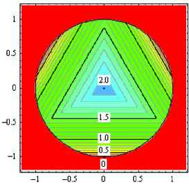
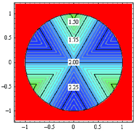
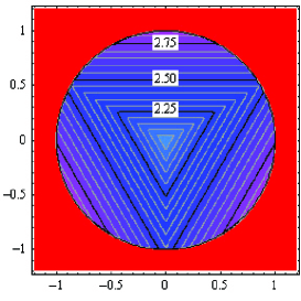
Figure 5: (a), (b), (c) density and contour plots for masses $M_{1}$, $M_{2}$, and $M_{3}$ of the lightest $N_{1}$, medium heavy $N_{2}$ and heaviest $N_{3}$ heavy neutrino respectively (TeV). The distances between two consecutive equipotential lines are $\Delta M_{1}=0.1$ TeV, $\Delta M_{2}=\Delta M_{3}=0.05$ TeV; (d) the vicinity of the point where $M_{1}$ approaches zero ($r=1$, $\theta=-\pi/2$); $\Delta\ M_{1}=0.025$ TeV; (e) mass color coding.

Now we have everything at hand to calculate the lifetimes of the heavy neutrinos in the Okamura model. The parameter space of the model is represented by the interior of a unit circle as discussed in section II. For each point inside the unit circle, we can calculate the Okamura texture using Eqs. (1), (7), (8), (10), and (11), diagonalize it to obtain the masses and mixings algorithm , and calculate the decay widths and lifetimes of the heavy neutrinos using Eq. (50). As the Higgs mass, we take $m_{H}=200$ GeV. (The choice of the Higgs mass has little effect on our result as long as $m_{H}\ll M_{i}$.)

The resulting contour and density plots for masses, decay widths, and lifetimes of the heavy neutrinos $N_{1}$, $N_{2}$ and $N_{3}$ are presented in Figs. 5–7. First, note that the graphs are symmetric under rotations by multiples of $2\pi/3$ as anticipated in section II. Next, from Fig. 5, we can easily see that the values of the heavy neutrino masses are larger than the $W$, $Z$, or Higgs thresholds for most of the parameter space, justifying our use of two-body decay amplitudes. The mass of $N_{1}$ becomes smaller than these thresholds only in the vicinity of three isolated points at $r=1$, $\theta=-\pi/2+2\pi k/3$ ($k=0,1,2$), as illustrated in Fig. 5d. As was shown in Ref. okamura , at these three points one of the $N$-fields is completely massless while the other two have degenerate mass. The lightest $N$ particle is completely stable at these points with zero decay width and infinite lifetime. However, the existence of such a light (less than $W$ and $Z$ thresholds) $N$ particle is already ruled out experimentally by L3 Achard:2001qv so we need not consider these points further.

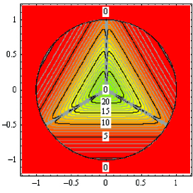
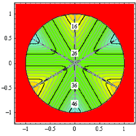
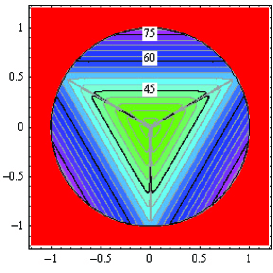
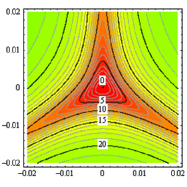
\begin{picture}(87.0,2.0)(0.0,0.0)\end{picture}

Figure 6: (a), (b), (c) density and contour plots for widths $\Gamma_{1}$, $\Gamma_{2}$, and $\Gamma_{3}$ of the lightest $N_{1}$, medium heavy $N_{2}$ and heaviest $N_{3}$ heavy neutrino respectively (GeV). The distances between two consecutive equipotential lines are $\Delta\Gamma_{1}=1$ GeV, $\Delta\Gamma_{2}=2$ GeV, $\Delta\Gamma_{3}=3$ GeV; (d) the detailed picture of the central part of $\Gamma_{1}$; $\Delta\Gamma_{1}=1$ GeV; (e) width color coding.

It was also shown in Ref. okamura that at the center of the circle one heavy neutrino completely decouples from the light neutrino states (and therefore from the rest of the Standard Model particles) while the other two heavy states have degenerate masses. This decoupling can be seen in Fig. 6d and Fig. 7d where at the center of the circle the decay width of the lightest heavy neutrino is zero and the lifetime is infinite. A similar decoupling occurs at the points where $r=1$ and $\theta=-5\pi/6+2\pi k/3$, $k=0,1,2$.

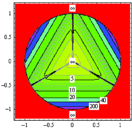
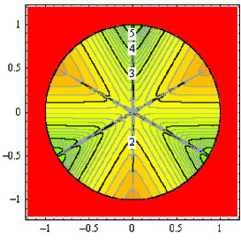
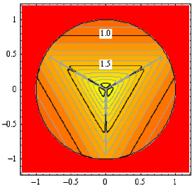
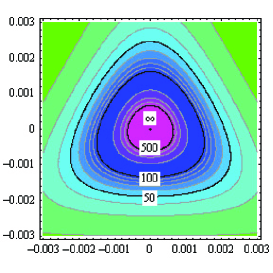
\begin{picture}(87.0,2.0)(0.0,0.0)\end{picture}

Figure 7: (a), (b), (c) density and contour plots for lifetimes $\tau_{1}$, $\tau_{2}$, and $\tau_{3}$ of the lightest $N_{1}$, medium heavy $N_{2}$ and heaviest $N_{3}$ heavy neutrino respectively ($10^{-26}$ sec). The distances between two consecutive equipotential lines are $\Delta\tau_{1}=1\times 10^{-26}$ sec for $\tau_{1}<10\times 10^{-26}$ sec and for $\tau_{1}>10\times 10^{-26}$ sec equipotential lines corresponding to $\tau_{1}=20\times 10^{-26}$, $40\times 10^{-26}$ and $200\times 10^{-26}$ sec are presented, $\Delta\tau_{2}=0.2\times 10^{-26}$ sec, $\Delta\tau_{3}=0.1\times 10^{-26}$ sec; (d) the detailed picture of the central part of $\tau_{1}$; $\Delta\tau_{1}=10\times 10^{-26}$ sec for $\tau_{1}<100\times 10^{-26}$ sec and $\Delta\tau_{1}=100\times 10^{-26}$ sec for $\tau_{1}>100\times 10^{-26}$ sec; (e) lifetime color coding.

Except for the vicinity of these points, the lifetimes of the $N$ particles are typically in the range of $10^{-26}$ to $10^{-24}$ seconds (see Fig. 7). Assuming that the particles are non-relativistic, the maximum distance they can travel from their production points before decay is in the range of $10^{-17}$ to $10^{-15}$ meters. If produced at colliders, they will decay inside the detector. On the other hand, the width-to-mass ratios of the particles are in the range of 0.1 to 3 percent as shown in Fig. 8. Therefore, the invariant mass spectrum of the decay products can be expected to show a very narrow peak.

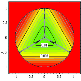
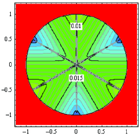
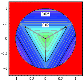
Figure 8: (a), (b), (c) density and contour plots for the widths-to-mass ratios of the lightest $N_{1}$, medium heavy $N_{2}$ and heaviest $N_{3}$ heavy neutrinos respectively. The distances between two consecutive equipotential lines is $0.001$ for all plots; (d) mass-to-width ratio color coding.

VI Summary and Discussion

In this paper, we calculate the mass spectrum, decay widths and lifetimes of the mostly-right-handed heavy neutrino states that appear in the model proposed by Okamura et al. in Ref. okamura . We map the parameter space of the Okamura model to the interior of a unit circle, and represent the results of our calculations as density-contour plots over it. For the phenomenologically viable region of the model’s parameter space, the heavy states have masses of a few TeV, and are short-lived with the typical lifetimes from $10^{-26}$ to $10^{-24}$ seconds. At the same time, the decay widths are very small comparing to the masses. The typical width-to-mass ratio is in the range of $0.1$ to $3$ percent.

Though we have found that the heavy neutral particles in the Okamura model have lifetimes in the range that allow for their observation at colliders, an analysis by Dicus, Karatas, and Roy Dicus:1991fk suggests that they may be difficult to observe at the LHC. In Ref. Dicus:1991fk , the authors consider the production of like-sign leptons, a lepton number violating process, as the signature of the heavy mostly-right-handed Majorana neutrino $N$: this can occur through the process $W^{\pm}\rightarrow\ell^{\pm}N\rightarrow\ell^{\pm}\ell^{\pm}W^{\mp}\rightarrow\ell^{\pm}\ell^{\pm}+\mbox{jets}$, or the $t$- and $u$-channel exchange of $N$ between two like-sign $W$’s radiated from the protons. Assuming masses in the range of $150\sim 4000$ GeV, and a mixing as large as $\theta^{2}\sim 0.043$ (an order of magnitude larger than the Okamura model), the number of expected events at the LHC was shown to be only a few per year; too few for them to be discernible above the Standard Model background.

If the gauge group is extended to $SU(2)_{L}\times SU(2)_{R}\times U(1)_{B-L}$, then the $N$’s can be copiously produced through the $W_{R}$ and $Z^{\prime}$, as discussed in Refs. Ho:1990dt ; Datta:1992qw ; ATLAS:1999fq . We will discuss the embedding of the Okamura texture into this gauge structure in a subsequent paper PT2 .

References

- (1) T. Yanagida, in Proceedings of the Workshop on Unified Theory and Baryon Number in the Universe, ed. O. Sawada and A. Sugamoto (KEK, report 79-18, 1979), p.95; M. Gell-Mann, P. Ramond and S. Slansky, in Supergravity, ed. P. van Nieuwenhuizen and D. Z. Freedman (North-Holland, Amsterdam, 1979), p315; R. N. Mohapatra and G. Senjanović, Phys. Rev. Lett. 44, 912 (1980).
- (2) W. Loinaz, N. Okamura, S. Rayyan, T. Takeuchi and L. C. R. Wijewardhana, Phys. Rev. D 68, 073001 (2003) [arXiv:hep-ph/0304004].
- (3) L. N. Chang, D. Ng and J. N. Ng, Phys. Rev. D 50, 4589 (1994) [arXiv:hep-ph/9402259].
- (4) C. D. Carone and H. Murayama, Phys. Lett. B 392, 403 (1997) [arXiv:hep-ph/9610383].
- (5) N. Arkani-Hamed, L. J. Hall, H. Murayama, D. R. Smith and N. Weiner, Phys. Rev. D 64, 115011 (2001) [arXiv:hep-ph/0006312].
- (6) E. Ma, Phys. Rev. Lett. 86, 2502 (2001) [arXiv:hep-ph/0011121].
- (7) [NuTeV Collaboration] G. P. Zeller et al., Phys. Rev. Lett. 88, 091802 (2002) [hep-ex/0110059]; Phys. Rev. D 65, 111103 (2002) [hep-ex/0203004]; K. S. McFarland et al., hep-ex/0205080; G. P. Zeller et al., hep-ex/0207052.
- (8) S. Davidson, S. Forte, P. Gambino, N. Rius and A. Strumia, JHEP 0202, 037 (2002) [hep-ph/0112302]; S. Davidson, hep-ph/0209316; P. Gambino, hep-ph/0211009.
- (9) W. Loinaz, N. Okamura, T. Takeuchi and L. C. R. Wijewardhana, Phys. Rev. D 67, 073012 (2003) [arXiv:hep-ph/0210193]; T. Takeuchi, arXiv:hep-ph/0209109.
- (10) S. Bilenky, C. Giunty, W. Grimus, arXiv:hep-ph/9812360.
- (11) J. C. Pati and A. Salam, Phys. Rev. D 8, 1240 (1973).
- (12) A. Denner, H. Eck, O. Hahn and J. Kublbeck, Nucl. Phys. B 387, 467 (1992).
- (13) A. Djouadi, Z. Phys. C 63, 317 (1994) [arXiv:hep-ph/9308339].
- (14) J. A. Aguilar-Saavedra, Int. J. Mod. Phys. C 8, 147 (1997) [arXiv:hep-ph/9607313].
- (15) P. Achard et al. [L3 Collaboration], Phys. Lett. B 517, 67 (2001) [arXiv:hep-ex/0107014].
- (16) D. A. Dicus, D. D. Karatas and P. Roy, Phys. Rev. D 44, 2033 (1991).
- (17) T. H. Ho, C. R. Ching and Z. J. Tao, Phys. Rev. D 42, 2265 (1990).
- (18) A. Datta, M. Guchait and D. P. Roy, Phys. Rev. D 47, 961 (1993) [arXiv:hep-ph/9208228].
- (19) ATLAS: Detector and physics performance technical design report, Volume 2, section 21.6.2 “Search for right-handed Majorana neutrinos”, CERN-LHCC-99-15 (May 25, 1999). Available from the CERN LHC website at http://atlas.web.cern.ch/Atlas/GROUPS/PHYSICS/TDR/access.html
- (20) A. Pronin and T. Takeuchi, in preparation.