QCD at hadron colliders

Abstract

QCD is an extensively developed and tested gauge theory, which models the strong interactions in the high-energy regime. In this talk, I shall review the considerable progress which has been achieved in the last few years in the most actively studied QCD topics: Monte Carlo models, higher-order corrections, and parton distribution functions. Thanks to that, QCD in the high-energy regime is becoming more and more an essential precision toolkit to analyse Higgs and New Physics scenarios at the LHC.

1. Introduction

Quantum chromodynamics (QCD) is by now widely accepted as the theory which describes the strong interactions between hadrons and their components, the quarks and gluons. From a theoretical point of view, it is a gauge field theory featuring asymptotic freedom, i.e. a coupling that grows weaker at smaller distances. However, the strong interactions also feature confinement, that is the lack of colour of the observed hadrons. Although in the non-perturbative (low $Q^{2}$) regime several clever approaches to QCD, like lattice gauge theory, Regge theory, chiral perturbation theory, large $N_{c}$, are used, a complete theoretical solution to confinement is not yet available and is difficult to obtain, because the QCD Lagrangian is formulated in terms of quarks and gluons, rather than the observed hadrons, and because at large distances, i.e. at low $Q^{2}$, the coupling is strong. Conversely, at small distances, i.e. in the high-energy regime, the coupling is weak and thus it is possible to make use of the perturbative framework. In this talk I shall focus on the fact that perturbative QCD (pQCD), i.e. QCD in the weak-coupling (high $Q^{2}$) regime, has emerged as an essential precision toolkit for exploring Higgs and Beyond-the-Standard-Model (BSM) physics; and that is even more so at the Large Hadron Collider (LHC), because of the strongly interacting colliding protons. In the box of the precision toolkit, pQCD provides the tools for a precise determination of the strong coupling constant, $\alpha_{\scriptscriptstyle S}$, of the parton distribution functions (p.d.f.), of the electroweak parameters and of the LHC parton luminosity; and of the strong corrections to Higgs and BSM signals and to their backgrounds.

In any scattering process in high-energy QCD, the value of any observable can be expanded in principle as a series in $\alpha_{\scriptscriptstyle S}$. Thus $\alpha_{\scriptscriptstyle S}$ represents the single most important piece of information we need. In the $\overline{\rm MS}$ scheme and using next-to-next-to-leading-order (NNLO) results only, the 2004 world average  [?] yields $\alpha_{\scriptscriptstyle S}(M_{Z})=0.1182\pm 0.0027$.

The fact that in the detectors experiments observe hadrons, while through the QCD Lagrangian we can only compute the scattering between partons, calls for a framework where the short-distance physics, which is responsible for the primary scattering between partons, can be separated from the long-distance physics, which describes the parton densities in the initial state and the hadronisation in the final state. That framework is provided by the pQCD and factorisation.

In the beginning there was the parton model and the Bjorken scaling, which constitute the backbone of pQCD. The latter computes the logarithmic scaling violations, that is the logarithmic corrections to the parton-model predictions. The pQCD tenets are the universality of the infrared (IR) behaviour, the cancellation of the IR singularities for suitably defined variables, like jets and event shapes, and in the case of hadron-initiated processes, like electron-proton or (anti)proton-proton collisions, the factorisation of the short- and long-range interactions.

Factorisation in proton-proton ($pp$) collisions states that the cross section for the production of high-mass states, like vector bosons, Higgs bosons, heavy quarks or large-$E_{T}$ jets, characterised by the large scale $Q^{2}$, can be expressed as a convolution of short- and long-distance pieces, with the matching between the two pieces occurring at an arbitrary scale $\mu_{F}$, called factorisation scale. The short-distance piece is the parton cross section for the primary event, describing how two partons out of the incoming protons collide to produce the high-mass states plus hard radiation; the long-distance pieces are the p.d.f.’s in the initial state (and eventually the fragmentation functions in the final state), describing the density of the colliding partons within the protons, and how that density changes with the parton virtuality and momentum fraction. The p.d.f.’s cannot be computed – they must be given by the experiment – but their dependence on $\mu_{F}$ can. If factorisation holds, the parton cross section may be computed as a power series in $\alpha_{\scriptscriptstyle S}$. The only limitation is then computational, and the state of the art is that some production rates with one (and very few with two) final-state particles are known at next-to-next-to-leading order (NNLO), while many with two and some with three (and for special cases with four) final-state particles are known at next-to-leading order (NLO). A matching accuracy is then required from the p.d.f.’s whose DGLAP evolution has been recently computed to NNLO  [?,?].

2. Breaking factorisation

Factorisation, though, ignores altogether the underlying event (UE), which can be operatively defined as whatever is in the $pp$ interaction besides the primary scattering. In particular, the UE includes the multiple-parton interactions as well as the interaction of spectator partons, i.e. other than the ones initiating the primary scattering, the assumption being that if such interactions occur they are characterised by a scale $\Lambda$ of the order of a GeV, and so they are suppressed by powers of $\Lambda^{2}/Q^{2}$ with respect to the primary scattering. Thus, the UE breaks factorisation by means of power-suppressed contributions. How important are they for a precision calculation ? There is no obvious answer to this question since of course we cannot use the pQCD framework to model the UE, and its analysis must rely solely upon the data. In $p\overline{p}$ collisions at the Tevatron, the UE is being studied  [?] by analysing in single-jet production the charged-particle multiplicity in regions which are perpendicular in azimuth to the jet, since that region is expected to be sensitive to the UE. The UE sensitivity to beam remnants and to multiple interactions can be reduced by selecting back-to-back two-jet topologies. A similar investigation is being planned also through the Drell-Yan production of vector bosons.

Other examples of factorisation-breaking contributions are: $a)$ the power corrections: Monte Carlo (MC) and theory modelling of power corrections were laid out and tested at LEP, where they also provided a determination of $\alpha_{S}$  [?]. However, those models still need be tested in hadron collisions: a study of single-jet production at the Tevatron running at two different centre-of-mass energies shows that the Bjorken scaling is violated more than logarithmically: data can fitted by assuming a power-correction shift in the jet $E_{T}$  [?]; $b)$ diffractive events  [?], which are known to violate factorisation at the Tevatron  [?,?].

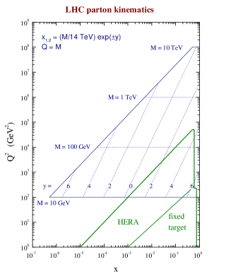
Figure  1.: LHC kinematic range, from MRST [10].

3. Monte Carlo models

The detection of Higgs and BSM signals requires a precise modelling of their backgrounds. Examples are QCD production of $W+4$ jets and of $WW+2$ jets, which are backgrounds to Higgs production through vector-boson fusion (VBF) with the Higgs decay into a $WW$ pair, as well to $t\overline{t}$ production, or $W+6$ jets and $WW+4$ jets, which are backgrounds to $Ht\overline{t}$ production. The huge amount of phase space available at the LHC, Fig. 1, as well as the large acceptance of the detectors, will make possible to produce final states with ten jets or more. One approach is to model QCD production through matrix-element MC generators, which provide an automatic computer generation of processes with many jets, and/or vector or Higgs bosons. There are several such multi-purpose generators, like e.g. ALPGEN  [?,?], ARIADNE  [?], MADGRAPH/MADEVENT  [?,?], COMPHEP  [?], GRACE/GR@PPA  [?,?], HELAC  [?], and SHERPA  [?] (which has got its own showering and hadronisation). A different example is PHASE/PHANTOM  [?], a MC generator dedicated to processes with six final-state partons only – thus suitable to $t\bar{t}$ production, $WW$ scattering, Higgs production via VBF and vector-boson gauge coupling studies, but where no approximation is used. Matrix-element MC generators are particularly suitable to studies which involve the geometry of the event, because the jets in the final state are generated at the matrix-element level, and thus exactly at any angle. In addition, they can be interfaced to parton-shower MC generators, like HERWIG  [?] or PYTHIA  [?], to include showering and hadronisation. In the context of matrix-element generators, the presence of several hard scales, like the mass of high-mass states, the jet transverse energy and the dijet invariant masses, makes an operative implementation of factorisation rather involved. The issue can be tackled through the CKKW  [?,?] (or CKKW-like  [?]) procedure. Within a given jet cross section, CKKW interfaces parton subprocesses with a different number of final states to parton showers.

Finally, MC@NLO  [?]: a procedure and a code to match exact NLO computations to shower MC generators. In a way, this is the most desirable procedure, because it embodies the precision of NLO parton calculations in predicting the overall normalisation of the event, while generating a realistic event set up through showering and hadronisation. It cannot be, though, multi-purpose, being obviously limited to the processes for which the NLO corrections are known.

4. NLO calculations

Another approach to the evaluation of the parton cross section $\hat{\sigma}$ is through fixed-order computations. These yield only a limited access to the final-state structure, but have the advantage that higher-order corrections, real and virtual, can be included exactly. The virtual corrections will depend on a fictitious scale $\mu_{R}$, at which the scattering amplitudes are renormalised to take care of the ultraviolet divergences. NLO calculations have several desirable features. $a)$ the jet structure: while in a leading-order calculation the jets have a trivial structure because each parton becomes a jet, to NLO the final-state collinear radiation allows up to two partons to enter a jet; $b)$ a more refined p.d.f. evolution through the initial-state collinear radiation; $c)$ the opening of new channels, through the inclusion of parton sub-processes which are not allowed to leading order; $d)$ a reduced sensitivity to the fictitious input scales $\mu_{R}$ and $\mu_{F}$ allows to predict the normalisation of physical observables, which is usually not accurate to leading order. That is the first step toward precision measurements in general, and in particular toward an accurate estimate of signal and background for Higgs and New Physics at LHC; $e)$ finally, the matching with a parton-shower MC generator, like MC@NLO, as mentioned in Sect. 3. .

Here we remind briefly how a NLO calculation is organised. Let us consider the production of $n$ jets in hadron collisions. There are two types of contributions to $\hat{\sigma}$: the tree-level production with $n+1$ final-state partons, with one of the partons that is undetected, and the one-loop production with $n$ final-state partons. Schematically,

$$\hat{\sigma}=\sigma^{\rm LO}+\sigma^{\rm NLO}=\int_{n}d\sigma^{B}+\sigma^{\rm NLO}$$ (1)

where $d\sigma^{B}$ is the Born cross section, and

$$\sigma^{\rm NLO}=\int_{n+1}d\sigma^{R}+\int_{n}d\sigma^{V}\ .$$ (2)

Both real and virtual contributions to Eq. (2), contain IR, i.e. collinear and soft, singularities. If in order to regulate those divergences one uses the dimensional regularisation, which fixes the dimensions of space-time to be $d=4-2\epsilon$, then one finds that both terms on the right-hand side of Eq. (2) are divergent at $d=4$. However, the structure of QCD is such that those singularities are universal, i.e. they do not depend on the process under consideration, but only on the partons involved in generating the singularity. Thus, in the 90’s process-independent procedures were devised to regulate those divergences. They are conventionally called slicing  [?,?], subtraction  [?,?] and dipole subtraction  [?], and use universal counterterms to subtract the divergences. The NLO contribution, Eq. (2), can be written as,

$$\sigma^{\rm NLO}=\int_{n+1}\left[(d\sigma^{R})_{\epsilon=0}-(d\sigma^{A})_{\epsilon=0}\right]+\int_{n}\left(d\sigma^{V}+\int_{1}d\sigma^{A}\right)\ ,$$ (3)

such that both sums of bracketed terms on the right-hand side of Eq. (3) are finite at $d=4$, and thus readily integrable numerically via a computer code, with arbitrary selection cuts on the final-state particles and jets, as eventually required by a detector simulation. The organisation of NLO computations in process-independent procedures has made them an essential tool in the comparison with the experimental data.

Let us look briefly at the history of NLO calculations: the first final-state distribution to NLO was computed for $e^{+}e^{-}\to$ 3 jets  [?]. The addition of just one more jet in the final state, to produce $e^{+}e^{-}\to$ 4 jets, took about 15 years  [?,?]. This trend, namely the great difficulty in adding one more jet to a given final-state distribution, is repeated in all the other NLO calculations: in Drell-Yan with one associated jet  [?], and with two associated jets  [?]; in one- or two-jet production in hadron collisions  [?,?], and in three-jet production  [?,?]; in di-photon production in hadron collisions  [?,?], and in the same with one associated jet  [?]. Conversely, for other distributions in hadron collisions, like heavy-quark pair production  [?], vector-boson pair production (including the spin correlations)  [?,?], Drell-Yan with a heavy-quark pair  [?], Higgs production via gluon fusion with one associated jet  [?,?], Higgs production via vector-boson fusion with two associated jets  [?], Higgs production with a heavy-quark pair  [?,?], the addition of just one more jet has not been achieved yet to NLO. Furthermore, all the hadron-initiated distributions above have no more than three final-state particles (only very special cases with four final-state particles, like the NLO corrections to the electroweak production of a vector-boson pair $+$ 2 jets  [?], are known).

Why in a NLO calculation is it so difficult to add more particles in the final state ? The loop integrals occurring in the virtual contributions to Eq. (2) are involved and process dependent. In addition, more final-state particles imply more scales in the process, and so lenghtier analytic expressions in the loop integral. In fact, the only known complete one-loop amplitudes with hexagon loops are the ones for six gluons  [?,?,?,?,?,?,?,?] and for the electroweak corrections to $e^{+}e^{-}\to 4$ fermions  [?]; with heptagon loops are the ones for seven gluons in N=4 super-yang-Mills theory  [?]. Recently, a twistor-inspired approach  [?], which has allowed for great advances in the analytic computation of tree and one-loop amplitudes  [?,?,?,?], as well as several semi-numerical approaches which show promise to handle NLO corrections in an automated way  [?,?,?,?,?,?,?,?,?], have appeared. However, the programme of applying sistematically NLO computations to studies of signals and backgrounds for Higgs and New Physics is still in its infancy and will be undoubtedly receive a lot of attention in the next future.

5. NNLO calculations

Are NLO computations accurate enough to describe the data ? The answer to that question is of course process dependent. Here I shall give a few examples:

• $b$ production at the Tevatron It has been long thought that the CDF data for $b$ quark production were not in agreement with the NLO prediction (for a historical overview, see Ref.  [?]). However, in the comparison of the CDF Run II data  [?] for the $J/\psi$ momentum distribution in inclusive $B\to J/\psi+X$ decays to the NLO prediction  [?] and to MC@NLO  [?], one finds that the data lie within the theory uncertainty band and are in good agreement with the theory predictions.

• $W$ production at the LHC The Drell-Yan $W$ cross section, with leptonic decay of the $W$ boson, has been proposed as a luminosity monitor of the LHC  [?], warranting a greater accuracy, of the order of a few percent, than the standard determination of the luminosity through the total hadronic cross section. However, the experimental $W$ cross section depends on the acceptance, i.e. the fraction of events which pass the selection cuts. Thus, the accuracy of the luminosity monitor, the standard candle, depends on the one of the acceptance, which is related to the precision by which the hard cross section is known. In Ref.  [?] the $W$ cross section has been computed to different accuracies: to leading order, the same $+$ HERWIG, NLO, MC@NLO, with or without including the spin correlations between the decay leptons and the partons entering the hard scattering. It was found that the difference between the NLO calculation and MC@NLO is about $2-3\%$, which is much less than the difference between the same calculations with and without spin correlations. Therefore, to whatever accuracy we may compute the $W$ cross section, if we want to use it as a standard candle it is mandatory to include the spin correlations. Recently, a calculation of the NNLO corrections, including the spin correlations, has been completed  [?]. It shows that the NNLO corrections differ from the NLO corrections more than $2-3\%$ only if severe acceptance cuts on the $p_{T}$ of the outgoing electron are used, which restrict drastically the available phase space.

• Higgs production at the LHC At hadron colliders, the leading production mode for the Higgs is via gluon-gluon fusion through the mediation of a heavy-quark (mostly top-quark) loop. The NLO corrections to fully inclusive Higgs production via gluon-gluon fusion, including the heavy-quark mass dependence, required an evaluation at two-loop accuracy, and were found to be as large  [?,?] as the leading-order calculation. That situation was unsatisfactory, because it called for a calculation to NNLO , which requires an evaluation at three-loop accuracy. However, in the large-$m_{t}$ limit, i.e. when the Higgs mass is smaller than the threshold for the creation of a top-quark pair, $m_{\scriptscriptstyle H}\mathrel{\mathchoice{\lower 3.0pt\vbox{\halign{$\m@th\displaystyle\hfill#\hfil$\cr<\crcr\sim\crcr}}}{\lower 3.0pt\vbox{\halign{$\m@th\textstyle\hfill#\hfil$\cr<\crcr\sim\crcr}}}{\lower 3.0pt\vbox{\halign{$\m@th\scriptstyle\hfill#\hfil$\cr<\crcr\sim\crcr}}}{\lower 3.0pt\vbox{\halign{$\m@th\scriptscriptstyle\hfill#\hfil$\cr<\crcr\sim\crcr}}}}2m_{t}$, the coupling of the Higgs to the gluons via a top-quark loop can be replaced by an effective coupling. That reduces the number of loops in a given diagram by one. The NNLO corrections have been evaluated in the large-$m_{t}$ limit  [?,?,?] and display a modest increase with respect to the NLO evaluation, showing that the calculation stabilises to NNLO.

In the examples above I stressed how the central value of a prediction may change when going from leading order to NLO and eventually to NNLO. However, a benefit of going from leading order to NLO and then to NNLO is the reduction of the theory uncertainty band, due to the lesser sensitivity to the fictitious input scales $\mu_{R}$ and $\mu_{F}$ of the calculation. Thus, a lot of theoretical activity has been directed in the last years toward the calculation of cross sections to NNLO accuracy. The total cross section  [?,?] and the rapidity distribution  [?,?] for Drell-Yan $W,Z$ production are known to NNLO accuracy. So are the total cross section  [?,?,?] and the rapidity distribution  [?] for Higgs production via gluon-gluon fusion, in the large-$m_{t}$ limit. However, only the calculation of Ref.  [?], which has been extended to include the di-photon background  [?], and Ref.  [?] allow the use of arbitrary selection cuts.

Basically, there are three ways of computing NNLO corrections:

• Analytic integration, which is the first method to have been used  [?], and may include a limited class of acceptance cuts by modelling cuts as “propagators”  [?,?]. Besides total cross sections, it has been used to produce the NNLO differential rates of Ref.  [?].

• Sector decomposition, which is flexible enough to include any acceptance cuts  [?,?,?,?], and has been used to produce the NNLO differential rates of Refs.  [?,?,?] and of $e^{+}e^{-}\to 2$ jets  [?]. The cancellation of the IR divergences is performed numerically.

• Subtraction, for which the cancellation of the divergences is organised in a process-independent way by exploiting the universal structure of the IR divergences, in particular the universal structure of the three-parton tree-level splitting functions  [?,?,?,?,?] and of the two-parton one-loop splitting functions  [?,?,?,?,?]. Although, the universal splitting functions have been known for some time, the cancellation of the IR divergences to NNLO is very intricate  [?,?,?,?,?,?,?,?,?], and except for test cases like $e^{+}e^{-}\to 2$ jets  [?,?] and for parts of $e^{+}e^{-}\to 3$ jets  [?], no NNLO numerical code has been devised yet.

6. The parton distribution functions

As outlined in the Introduction, at hadron colliders the theory cross section can be written using factorisation as a convolution of the parton cross section with the p.d.f.’s. The dependence of the p.d.f.’s on $Q^{2}$ is given by the DGLAP evolution equations. In those equations, the evolution in $Q^{2}$ is driven by the splitting functions, which are perturbatively computable. By consistency, in the factorisation formula the parton cross section and the splitting functions must be determined to the same accuracy. The leading-order  [?,?] and NLO  [?] splitting functions have been known for a long time. The calculation of the NNLO splitting functions has been completed recently  [?,?], setting the record as the toughest calculation ever performed in perturbative QCD: it took the equivalent of 20 man-years, and about a million lines of dedicated algebra code. The p.d.f.’s obtained by global fits  [?] of all accessible collider and fixed-target data can be evolved to the large kinematic range accessible through the LHC. In global fits, the fit is performed by minimising the $\chi^{2}$ to all the data. The evolution is started at some value $Q^{2}_{0}$, where the p.d.f. is some suitable function of $x$. In addition, to avoid higher-twist contaminations, the data are selected above a certain momentum transfer and energy, $Q^{2}>Q^{2}_{\rm min}$ and $W^{2}>W^{2}_{\rm min}$. Recently, though, also an evaluation of the $\Delta\chi^{2}$, i.e. of the uncertainties arising from the errors on the experimental data, has been performed  [?,?,?,?,?], using either the Hessian or the Lagrange-multiplier methods.

7. Conclusions

QCD in the high-energy regime is constantly making progress. Here I have reviewed the considerable advances achieved in the last few years in the sectors of QCD which are most actively studied: Monte Carlo models, higher-order corrections and p.d.f.’s. More progress can be anticipated in modelling the underlying event, in improving the factorisation picture in Monte Carlo models through the use of CKKW-like procedures, in the automatisation of NLO calculations, and in a working NNLO numerical code based on subtraction, thus making high-energy QCD more and more an essential precision toolkit to analyse Higgs and New Physics scenarios at the LHC.

REFERENCES

- [1] S. Bethke, Nucl. Phys. Proc. Suppl. 135 (2004) 345 [hep-ex/0407021].
- [2] S. Moch, J. A. M. Vermaseren and A. Vogt, Nucl. Phys. B 688 (2004) 101 [hep-ph/0403192].
- [3] A. Vogt, S. Moch and J. A. M. Vermaseren, Nucl. Phys. B 691 (2004) 129 [hep-ph/0404111].
- [4] D. Acosta et al. [CDF Collaboration], Phys. Rev. D 70 (2004) 072002 [hep-ex/0404004].
- [5] Y. L. Dokshitzer, G. Marchesini and B. R. Webber, Nucl. Phys. B 469 (1996) 93 [hep-ph/9512336].
- [6] M.L. Mangano, presented at the KITP Collider Physics Conference, January 2004, http://online.kitp.ucsb.edu/online/collider_ c04/mangano/
- [7] J. C. Collins, L. Frankfurt and M. Strikman, Phys. Lett. B 307 (1993) 161 [hep-ph/9212212].
- [8] K. Terashi [CDF Collaboration], Int. J. Mod. Phys. A 16S1A (2001) 265.
- [9] D. Acosta et al. [CDF Collaboration], Phys. Rev. Lett. 93 (2004) 141601 [hep-ex/0311023].
- [10] A. D. Martin, R. G. Roberts, W. J. Stirling and R. S. Thorne, Eur. Phys. J. C 14 (2000) 133 [hep-ph/9907231].
- [11] M. L. Mangano, M. Moretti and R. Pittau, Nucl. Phys. B 632 (2002) 343 [hep-ph/0108069].
- [12] M. L. Mangano, M. Moretti, F. Piccinini, R. Pittau and A. D. Polosa, JHEP 0307 (2003) 001 [hep-ph/0206293].
- [13] L. Lonnblad, Comput. Phys. Commun. 71 (1992) 15.
- [14] T. Stelzer and W. F. Long, Comput. Phys. Commun. 81 (1994) 357 [hep-ph/9401258].
- [15] F. Maltoni and T. Stelzer, JHEP 0302 (2003) 027 [hep-ph/0208156].
- [16] A. Pukhov et al., hep-ph/9908288.
- [17] T. Ishikawa, T. Kaneko, K. Kato, S. Kawabata, Y. Shimizu and H. Tanaka [MINAMI-TATEYA group Collaboration], KEK-92-19
- [18] F. Yuasa et al., Prog. Theor. Phys. Suppl. 138 (2000) 18 [hep-ph/0007053].
- [19] A. Kanaki and C. G. Papadopoulos, Comput. Phys. Commun. 132 (2000) 306 [hep-ph/0002082].
- [20] F. Krauss, A. Schalicke, S. Schumann and G. Soff, Phys. Rev. D 70 (2004) 114009 [hep-ph/0409106].
- [21] E. Accomando, A. Ballestrero and E. Maina, Nucl. Instrum. Meth. A 534 (2004) 265 [hep-ph/0404236].
- [22] G. Marchesini, B. R. Webber, G. Abbiendi, I. G. Knowles, M. H. Seymour and L. Stanco, Comput. Phys. Commun. 67 (1992) 465.
- [23] T. Sjostrand, Comput. Phys. Commun. 82 (1994) 74.
- [24] S. Catani, F. Krauss, R. Kuhn and B. R. Webber, JHEP 0111 (2001) 063 [hep-ph/0109231].
- [25] F. Krauss, JHEP 0208 (2002) 015 [hep-ph/0205283].
- [26] S. Hoche, F. Krauss, N. Lavesson, L. Lonnblad, M. Mangano, A. Schalicke and S. Schumann, hep-ph/0602031.
- [27] S. Frixione and B. R. Webber, JHEP 0206 (2002) 029 [hep-ph/0204244].
- [28] W. T. Giele and E. W. N. Glover, Phys. Rev. D 46 (1992) 1980.
- [29] W. T. Giele, E. W. N. Glover and D. A. Kosower, Nucl. Phys. B 403 (1993) 633 [hep-ph/9302225].
- [30] S. Frixione, Z. Kunszt and A. Signer, Nucl. Phys. B 467 (1996) 399 [hep-ph/9512328].
- [31] Z. Nagy and Z. Trocsanyi, Nucl. Phys. B 486 (1997) 189 [hep-ph/9610498].
- [32] S. Catani and M. H. Seymour, Nucl. Phys. B 485 (1997) 291 [Erratum-ibid. B 510 (1997) 291] [hep-ph/9605323].
- [33] R. K. Ellis, D. A. Ross and A. E. Terrano, Nucl. Phys. B 178 (1981) 421.
- [34] L. J. Dixon and A. Signer, Phys. Rev. D 56, 4031 (1997) [hep-ph/9706285].
- [35] Z. Nagy and Z. Trocsanyi, Phys. Rev. Lett. 79 (1997) 3604 [hep-ph/9707309].
- [36] J. Campbell and R. K. Ellis, Phys. Rev. D 65 (2002) 113007 [hep-ph/0202176].
- [37] S. D. Ellis, Z. Kunszt and D. E. Soper, Phys. Rev. Lett. 64 (1990) 2121.
- [38] W. B. Kilgore and W. T. Giele, hep-ph/9903361.
- [39] Z. Nagy, Phys. Rev. Lett. 88 (2002) 122003 [hep-ph/0110315].
- [40] B. Bailey, J. F. Owens and J. Ohnemus, Phys. Rev. D 46 (1992) 2018.
- [41] T. Binoth, J. P. Guillet, E. Pilon and M. Werlen, Eur. Phys. J. C 16 (2000) 311 [hep-ph/9911340].
- [42] V. Del Duca, F. Maltoni, Z. Nagy and Z. Trocsanyi, JHEP 0304 (2003) 059 [hep-ph/0303012].
- [43] M. L. Mangano, P. Nason and G. Ridolfi, Nucl. Phys. B 373 (1992) 295.
- [44] J. M. Campbell and R. K. Ellis, Phys. Rev. D 60 (1999) 113006 [hep-ph/9905386].
- [45] L. J. Dixon, Z. Kunszt and A. Signer, Phys. Rev. D 60 (1999) 114037 [hep-ph/9907305].
- [46] D. de Florian, M. Grazzini and Z. Kunszt, Phys. Rev. Lett. 82 (1999) 5209 [hep-ph/9902483].
- [47] C. J. Glosser and C. R. Schmidt, JHEP 0212 (2002) 016 [hep-ph/0209248].
- [48] T. Figy, C. Oleari and D. Zeppenfeld, Phys. Rev. D 68 (2003) 073005 [hep-ph/0306109].
- [49] W. Beenakker, S. Dittmaier, M. Kramer, B. Plumper, M. Spira and P. M. Zerwas, Phys. Rev. Lett. 87 (2001) 201805 [hep-ph/0107081].
- [50] L. Reina and S. Dawson, Phys. Rev. Lett. 87 (2001) 201804 [hep-ph/0107101].
- [51] B. Jager, C. Oleari and D. Zeppenfeld, hep-ph/0603177; hep-ph/0604200.
- [52] Z. Bern, L. J. Dixon, D. C. Dunbar and D. A. Kosower, Nucl. Phys. B 425 (1994) 217 [hep-ph/9403226]; Nucl. Phys. B 435 (1995) 59 [hep-ph/9409265].
- [53] S. J. Bidder, N. E. J. Bjerrum-Bohr, L. J. Dixon and D. C. Dunbar, Phys. Lett. B 606 (2005) 189 [hep-th/0410296].
- [54] S. J. Bidder, N. E. J. Bjerrum-Bohr, D. C. Dunbar and W. B. Perkins, Phys. Lett. B 608 (2005) 151 [hep-th/0412023].
- [55] R. Britto, E. Buchbinder, F. Cachazo and B. Feng, Phys. Rev. D 72 (2005) 065012 [hep-ph/0503132].
- [56] Z. Bern, N. E. J. Bjerrum-Bohr, D. C. Dunbar and H. Ita, JHEP 0511 (2005) 027 [hep-ph/0507019].
- [57] R. Britto, B. Feng and P. Mastrolia, Phys. Rev. D 73 (2006) 105004 [hep-ph/0602178].
- [58] R. K. Ellis, W. T. Giele and G. Zanderighi, JHEP 0605 (2006) 027 [hep-ph/0602185].
- [59] C. F. Berger, Z. Bern, L. J. Dixon, D. Forde and D. A. Kosower, hep-ph/0604195.
- [60] A. Denner, S. Dittmaier, M. Roth and L. H. Wieders, Phys. Lett. B 612 (2005) 223 [hep-ph/0502063].
- [61] Z. Bern, V. Del Duca, L. J. Dixon and D. A. Kosower, Phys. Rev. D 71 (2005) 045006 [hep-th/0410224].
- [62] E. Witten, Commun. Math. Phys. 252 (2004) 189 [hep-th/0312171].
- [63] F. Cachazo, P. Svrcek and E. Witten, JHEP 0409 (2004) 006 [hep-th/0403047].
- [64] R. Britto, F. Cachazo, B. Feng and E. Witten, Phys. Rev. Lett. 94 (2005) 181602 [hep-th/0501052].
- [65] Z. Bern, L. J. Dixon and D. A. Kosower, Phys. Rev. D 71 (2005) 105013 [hep-th/0501240]; Phys. Rev. D 73 (2006) 065013 [hep-ph/0507005].
- [66] D. A. Kosower, these proceedings.
- [67] M. Kramer and D. E. Soper, Phys. Rev. D 66 (2002) 054017 [hep-ph/0204113].
- [68] T. Binoth, G. Heinrich and N. Kauer, Nucl. Phys. B 654 (2003) 277 [hep-ph/0210023].
- [69] Z. Nagy and D. E. Soper, JHEP 0309 (2003) 055 [hep-ph/0308127].
- [70] W. T. Giele and E. W. N. Glover, JHEP 0404 (2004) 029 [hep-ph/0402152].
- [71] T. Binoth, J. P. Guillet, G. Heinrich, E. Pilon and C. Schubert, JHEP 0510 (2005) 015 [hep-ph/0504267].
- [72] R. K. Ellis, W. T. Giele and G. Zanderighi, Phys. Rev. D 72 (2005) 054018 [hep-ph/0506196]; Phys. Rev. D 73 (2006) 014027 [hep-ph/0508308].
- [73] C. Anastasiou and A. Daleo, hep-ph/0511176.
- [74] M. Czakon, hep-ph/0511200.
- [75] T. Binoth, M. Ciccolini and G. Heinrich, Nucl. Phys. Proc. Suppl. 157 (2006) 48 [hep-ph/0601254].
- [76] M. L. Mangano, AIP Conf. Proc. 753 (2005) 247 [hep-ph/0411020].
- [77] D. Acosta et al. [CDF Collaboration], Phys. Rev. D 71 (2005) 032001 [hep-ex/0412071].
- [78] M. Cacciari, S. Frixione, M. L. Mangano, P. Nason and G. Ridolfi, JHEP 0407 (2004) 033 [hep-ph/0312132].
- [79] S. Frixione, P. Nason and B. R. Webber, JHEP 0308 (2003) 007 [hep-ph/0305252].
- [80] M. Dittmar, F. Pauss and D. Zurcher, Phys. Rev. D 56 (1997) 7284 [hep-ex/9705004].
- [81] S. Frixione and M. L. Mangano, JHEP 0405 (2004) 056 [hep-ph/0405130].
- [82] K. Melnikov and F. Petriello, hep-ph/0603182.
- [83] D. Graudenz, M. Spira and P. M. Zerwas, Phys. Rev. Lett. 70 (1993) 1372.
- [84] M. Spira, A. Djouadi, D. Graudenz and P. M. Zerwas, Nucl. Phys. B 453 (1995) 17 [hep-ph/9504378].
- [85] C. Anastasiou, K. Melnikov and F. Petriello, Phys. Rev. Lett. 93 (2004) 262002 [hep-ph/0409088].
- [86] R. V. Harlander and W. B. Kilgore, Phys. Rev. Lett. 88 (2002) 201801 [hep-ph/0201206].
- [87] C. Anastasiou and K. Melnikov, Nucl. Phys. B 646 (2002) 220 [hep-ph/0207004].
- [88] V. Ravindran, J. Smith and W. L. van Neerven, Nucl. Phys. B 665 (2003) 325 [hep-ph/0302135].
- [89] R. Hamberg, W. L. van Neerven and T. Matsuura, Nucl. Phys. B 359 (1991) 343 [Erratum-ibid. B 644 (2002) 403].
- [90] C. Anastasiou, L. J. Dixon, K. Melnikov and F. Petriello, Phys. Rev. Lett. 91 (2003) 182002 [hep-ph/0306192].
- [91] C. Anastasiou, L. J. Dixon, K. Melnikov and F. Petriello, Phys. Rev. D 69 (2004) 094008 [hep-ph/0312266].
- [92] C. Anastasiou and K. Melnikov, Phys. Rev. D 67 (2003) 037501 [hep-ph/0208115].
- [93] C. Anastasiou, K. Melnikov and F. Petriello, Nucl. Phys. B 724 (2005) 197 [hep-ph/0501130].
- [94] M. Roth and A. Denner, Nucl. Phys. B 479 (1996) 495 [hep-ph/9605420].
- [95] T. Binoth and G. Heinrich, Nucl. Phys. B 585 (2000) 741 [hep-ph/0004013]; Nucl. Phys. B 693 (2004) 134 [hep-ph/0402265].
- [96] G. Heinrich, Nucl. Phys. Proc. Suppl. 116 (2003) 368 [hep-ph/0211144]; hep-ph/0601062.
- [97] C. Anastasiou, K. Melnikov and F. Petriello, Phys. Rev. D 69 (2004) 076010 [hep-ph/0311311].
- [98] C. Anastasiou, K. Melnikov and F. Petriello, Phys. Rev. Lett. 93 (2004) 032002 [hep-ph/0402280].
- [99] F. A. Berends and W. T. Giele, Nucl. Phys. B 313 (1989) 595.
- [100] A. Gehrmann-De Ridder and E. W. N. Glover, Nucl. Phys. B 517 (1998) 269 [hep-ph/9707224].
- [101] J. M. Campbell and E. W. N. Glover, Nucl. Phys. B 527 (1998) 264 [hep-ph/9710255].
- [102] S. Catani and M. Grazzini, Phys. Lett. B 446 (1999) 143 [hep-ph/9810389]; Nucl. Phys. B 570 (2000) 287 [hep-ph/9908523].
- [103] V. Del Duca, A. Frizzo and F. Maltoni, Nucl. Phys. B 568 (2000) 211 [hep-ph/9909464].
- [104] Z. Bern, L. J. Dixon, D. C. Dunbar and D. A. Kosower, Nucl. Phys. B 425 (1994) 217 [hep-ph/9403226].
- [105] Z. Bern, V. Del Duca and C. R. Schmidt, Phys. Lett. B 445 (1998) 168 [hep-ph/9810409].
- [106] D. A. Kosower, Nucl. Phys. B 552 (1999) 319 [hep-ph/9901201].
- [107] D. A. Kosower and P. Uwer, Nucl. Phys. B 563 (1999) 477 [hep-ph/9903515].
- [108] Z. Bern, V. Del Duca, W. B. Kilgore and C. R. Schmidt, Phys. Rev. D 60 (1999) 116001 [hep-ph/9903516].
- [109] D. A. Kosower, Phys. Rev. D 67 (2003) 116003 [hep-ph/0212097]; Phys. Rev. Lett. 91 (2003) 061602 [hep-ph/0301069]; Phys. Rev. D 71 (2005) 045016 [hep-ph/0311272].
- [110] S. Weinzierl, JHEP 0303 (2003) 062 [hep-ph/0302180]; JHEP 0307 (2003) 052 [hep-ph/0306248].
- [111] A. Gehrmann-De Ridder, T. Gehrmann and G. Heinrich, Nucl. Phys. B 682 (2004) 265 [hep-ph/0311276].
- [112] A. Gehrmann-De Ridder, T. Gehrmann and E. W. N. Glover, Nucl. Phys. B 691 (2004) 195 [hep-ph/0403057].
- [113] A. Gehrmann-De Ridder, T. Gehrmann and E. W. N. Glover, Phys. Lett. B 612 (2005) 36 [hep-ph/0501291]; Phys. Lett. B 612 (2005) 49 [hep-ph/0502110].
- [114] S. Frixione and M. Grazzini, JHEP 0506 (2005) 010 [hep-ph/0411399].
- [115] G. Somogyi, Z. Trocsanyi and V. Del Duca, JHEP 0506 (2005) 024 [hep-ph/0502226].
- [116] A. Gehrmann-De Ridder, T. Gehrmann and E. W. N. Glover, JHEP 0509 (2005) 056 [hep-ph/0505111].
- [117] S. Weinzierl, hep-ph/0606008.
- [118] D. J. Gross and F. Wilczek, Phys. Rev. D 8 (1973) 3633.
- [119] G. Altarelli and G. Parisi, Nucl. Phys. B 126 (1977) 298.
- [120] G. Curci, W. Furmanski and R. Petronzio, Nucl. Phys. B 175 (1980) 27.
- [121] A. D. Martin, R. G. Roberts, W. J. Stirling and R. S. Thorne, Phys. Lett. B 531 (2002) 216 [hep-ph/0201127].
- [122] D. Stump et al., Phys. Rev. D 65 (2002) 014012 [hep-ph/0101051].
- [123] J. Pumplin et al., Phys. Rev. D 65 (2002) 014013 [hep-ph/0101032].
- [124] J. Pumplin, D. R. Stump, J. Huston, H. L. Lai, P. Nadolsky and W. K. Tung, JHEP 0207 (2002) 012 [hep-ph/0201195].
- [125] A. D. Martin, R. G. Roberts, W. J. Stirling and R. S. Thorne, Eur. Phys. J. C 28 (2003) 455 [hep-ph/0211080].
- [126] A. D. Martin, R. G. Roberts, W. J. Stirling and R. S. Thorne, Eur. Phys. J. C 35 (2004) 325 [hep-ph/0308087].