Calculation of the Branching Ratio of $B^{-}\to h_{c}+K^{-}$ in PQCD

Abstract

The branching ratio of $B^{-}\rightarrow h_{c}+K^{-}$ is re-evaluated in the PQCD approach. In this theoretical framework all the phenomenological parameters in the wavefunctions and Sudakov factor are priori fixed by fitting other experimental data, and in the whole numerical computations we do not introduce any new parameter. Our results are consistent with the upper bounds set by the Babar and Belle measurements.

I introduction

$h_{c}$ of ${}^{1}P_{1}$ is the spin-partner of $\eta_{c}$ in the charmomium family, however, it seems to $h_{c}$ behaves very differently from other family members. Searching for $h_{c}$, as well as $h_{b}$ is a challenging task for both experimentalists and theorists of high energy physics barnes . $h_{c}$ was first seen at the CERN Intersecting Storage Rings (ISR) cern-isr , and later the E760 group at Fermilab reported observation of $h_{c}$ by studying the $p\bar{p}\to h_{c}\to\pi^{0}J/\psi$ fermilab-E760 . However, the E835 group claimed that they did not see $h_{c}$ in this channel. Instead, E835 reported observation of $h_{c}$ in another channel $p\bar{p}\to h_{c}\to\gamma\eta_{c}\to\gamma\gamma\gamma$ fermilab-E835 . Recently, the Babar collaboration set an upper bound for the production rate of $h_{c}$ as $3.4\times 10^{-6}$ for $BR(B^{-}\to h_{c}K^{-})\times BR(h_{c}\to J/\psi\pi^{+}\pi^{-})$ at $90\%$ C.L. Babar-hc . By contrast, the Belle collaboration reported null result on searching for $h_{c}$ via $B^{\pm}\to h_{c}K^{\pm}$ and gave an upper bound on the branching ratio as $BR(B^{+}\to h_{c}K^{+})<3.8\times 10^{-5}$ Belle-hc . The CLEO Collaboration has announced observation of $h_{c}$ in the decay $\psi(2S)\to\pi^{0}h_{c}\to\pi^{0}\gamma\eta_{c}$ with a very small branching ratio hc-CLEO-1 ; hc-CLEO-2 . As a comparison, so far, the BES II collaboration has not seen $h_{c}$ yet, and searching for it may be an important issue for the upgraded stage BES III.

One needs to understand the experimental status about the production rate of $h_{c}$. Moreover, a relatively larger production rate may be associated to new physics Demin ; Aydin ; Bi , therefore study on $h_{c}$ production may provide a chance to investigate effects of new physics, such as supersymmetry at lower energy scales. Of course, before invoking for new physics, one needs to more accurately estimate the production rate of $h_{c}$ in the standard model (SM).

Suzuki suggested to look for $h_{c}$ at $B^{+}\to h_{c}K^{+}\to\gamma\eta_{c}K^{+}\to\gamma(K\bar{K}\pi)K^{+}$ and if approximately $BR(B^{+}\to h_{c}K^{+})\approx BR(B^{+}\to\chi_{c0}K^{+})$, he estimated the cascade branching ratio as $2\times 10^{-5}$ suzuki . Gu considered another decay chain and estimated the branching ratio $BR(B^{+}\to h_{c}K^{+}\to\gamma\eta_{c}K^{+}\to\gamma(K_{S}^{0}K^{+}\pi^{-}+c.c.)K^{+}\to\gamma(\pi^{+}\pi^{-}K^{+}\pi^{-}+c.c.)K^{+})$ as $3.5\times 10^{-6}$gu .

In the decay of B-meson into charmonium is the so-called internal emission process where due to the color matching the process is suppressed compared to the external emission. Moreover, the non-factorizable effects would further change the contribution of the internal process besides a color factor of 1/3 Cheng . Therefore it seems that the smallness of $B\rightarrow h_{c}+K$ is natural. However, one could not reproduce experimental value of the $B^{-}\to\chi_{c0}K^{-}$ decay rate colangelo 1 in the QCD improved factorization, so that the authors of colangelo 1 suggested to consider re-scattering effects in B meson decay. They claimed that colangelo 1 a larger branching ratio for $B^{-}\to\chi_{c0}K^{-}$ which is consistent with data, was obtained. Motivated by the same idea, they applied the same scenario to investigate the re-scattering effects for $B^{-}\to h_{c}K^{-}$ case, i.e. supposing that the decay $B^{-}\to h_{c}K^{-}$ occurs via the the subsequent re-scattering effect of $D_{s}^{(*)}-D^{(*)0}$, the products of decay $B^{-}\to D_{s}^{(*)}D^{(*)0}$ colangelo 2 . They obtained a branching ratio ($BR(B^{-}\to h_{c}K^{-})=(2\sim 10)\times 10^{-4}$) which is much larger than the upper bound set by the Belle collaboration. It is very possible that the branching ratio of $B^{-}\to h_{c}K^{-}$ was overestimated in their work due to uncontrollable theoretical uncertainties, such as some input parameters and basic assumptions adopted in their calculation, which were comprehensively discussed in their paper.

Even though we may suppose that we have full knowledge on the weak and strong interactions at the quark level and can derive the quark-transition amplitude, the most difficult part is evaluation of the hadronic matrix elements of the exclusive processes. In fact, at present, a complete calculation of $B^{\pm}\to h_{c}K^{\pm}$ based on an underlying theoretical framework is absent. The perturbative QCD (PQCD) approach is believed to be successful for estimating transition rates of B and D into light mesons pqcd classic , even though there is still dispute about its applicability Sachrajda . The authors of ref. hc-amplitude applied the PQCD approach to study $B^{-}\to\chi_{c0}K^{-}$ and also obtained results which satisfactory comply with data. Therefore we have reason to believe that it is appropriate to analyze $B^{\pm}\to h_{c}K^{\pm}$ in this framework. In this work, we calculate decay rate of $B^{-}\to h_{c}K^{-}$ in the PQCD.

Generally, for two-body non-leptonic decays of B meson, both factorizable and non-factorizable diagrams contribute to the transition amplitudes, however, for $B^{-}\to h_{c}K^{-}$, the contributions from factorizable diagrams disappear since the conservation of G parity leads to $\langle 0|\bar{c}\gamma_{\mu}\gamma_{5}c|h_{c}\rangle=0$ K.C. Yang . Therefore, the decay rate of $B^{\pm}\to h_{c}K^{\pm}$ is much different from that in $B^{\pm}\to J/\psi K^{\pm}$ psi ; hc-amplitude where both factorizable and non-factorizable diagrams contribute.

To be more precise than the qualitative understanding, one needs to calculate the non-factorizable contribution where the QCD effects are accounted. Moreover, since the process is not factorizable, the convolution integral would involve the initial B-meson and all the two produced mesons altogether.

Our numerical results indeed indicate that the order of magnitude of $B^{-}\to h_{c}K^{-}$ should be of order of $3.6\times 10^{-5}$, which is smaller than the upper bound set by the Babar collaboration Babar-hc and slightly below the upper bound given by the Belle collaboration Belle-hc . It is noticed that our result about $B(B^{-}\to h_{c}K^{-})$ is smaller than that estimated by the authors of suzuki ; gu ; colangelo 1 and more consistent with data.

Indeed, more decisive conclusion should be made as more accurate data are accumulated by BES III, CLEO, Babar, Belle and even the LHCb.

The structure of this paper is organized as follows. After this introduction, we formulate the decay amplitude of $B^{-}\to h_{c}K^{-}$ in the PQCD approach. Then we present our numerical results along with all the input parameters in Sect. III. The last section is devoted to our conclusion and discussion. Some tedious expressions are collected in the Appendix.

II Formulation

The quark-diagrams which contribute to the transition amplitude of $B^{-}\to(^{1}P_{1})h_{c}+K^{-}$ are displayed in Fig. 1. As has been discussed in the introduction, the factorized diagrams Fig. 1 (a),(b) do not contribute to the amplitude because the the G parities of axial meson $h_{c}$ and axial current are mismatched and in the flavor SU(3) symmetry limit, the corresponding hadronic matrix element is forbiddencolangelo 1 ; K.C. Yang .

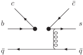
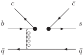
(a)						(b)
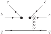
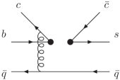
(c)						(d)

Figure 1: Feynman diagrams correspond to the calculation of hard amplitudes in $B\to h_{c}K$.

The effective Hamiltonian relevant to $B^{-}\to h_{c}K^{-}$ decay in the SM is written as effective-H

$$\mathcal{H}_{eff}=\frac{G_{F}}{\sqrt{2}}\bigg{[}V_{cb}V_{cs}^{*}\big{(}\mathcal{C}_{1}(\mu)\mathcal{O}_{1}+\mathcal{C}_{2}(\mu)\mathcal{O}_{2}\big{)}-V_{tb}V_{ts}^{*}\sum^{10}_{i=3}\mathcal{C}_{i}(\mu)\mathcal{O}_{i}\bigg{]},$$ (1)

where $C_{i}(\mu)$ are the Wilson coefficients and $\mathcal{O}_{i}$ are the relevant operators defined as

$$\mathcal{O}_{1} = (\bar{s}_{\alpha}c_{\beta})_{V-A}(\bar{c}_{\beta}b_{\alpha})_{V-A},\;\;\;\mathcal{O}_{2}=(\bar{s}_{\alpha}c_{\alpha})_{V-A}(\bar{c}_{\beta}b_{\beta})_{V-A},$$

$$\mathcal{O}_{3(5)} = (\bar{s}_{\alpha}b_{\alpha})_{V-A}\sum_{q}(\bar{q}_{\beta}q_{\beta})_{V-A(V+A)},\;\;\;\mathcal{O}_{4(6)}=(\bar{s}_{\alpha}b_{\beta})_{V-A}\sum_{q}(\bar{q}_{\beta}q_{\alpha})_{V-A(V+A)},$$

$$\mathcal{O}_{7(9)} = \frac{3}{2}(\bar{s}_{\alpha}b_{\alpha})_{V-A}\sum_{q}e_{q}(\bar{q}_{\beta}q_{\beta})_{V+A(V-A)},\;\;\;\mathcal{O}_{8(10)}=\frac{3}{2}(\bar{s}_{\alpha}b_{\beta})_{V-A}\sum_{q}e_{q}(\bar{q}_{\beta}q_{\alpha})_{V+A(V-A)},$$

with $\alpha$, $\beta$ being the color indices. The explicit expressions of the Wilson coefficients appearing in the above equations can be found in Ref. effective-H .

We define, in the rest frame of the B meson, $p$, $p^{\prime}$ and $q$ to be the four-moneta of $B$, $K$ and $h_{c}$, $k_{1(2)}$, $k_{1(2)}^{\prime}$ and $q_{1(2)}$ to be the momenta of the valence quarks inside B($b(\bar{q})$), $K$ ($s(\bar{q})$ ), and $h_{c}$ ($c(\bar{c})$ ), respectively. Then we parameterize the light cone momenta with all the light quarks and mesons being treated as massless

$$p = \frac{m_{B}}{\sqrt{2}}(1,1,\mathbf{0}_{\mathrm{T}})=(p^{+},p^{-},\mathbf{0}_{\mathrm{T}}),\qquad p^{\prime}=\frac{m_{B}}{\sqrt{2}}(0,1-r^{2},\mathbf{0}_{\mathrm{T}}),\qquad q=\frac{m_{B}}{\sqrt{2}}(1,r^{2},\mathbf{0}_{\mathrm{T}})=(q^{+},q^{-},\mathbf{0}_{\mathrm{T}}),$$

$$k_{1} = {(x_{1}p^{+},p^{-},\mathbf{k}_{1\mathrm{T}})},\qquad k_{2}={(\bar{x}_{1}p^{+},0,-\mathbf{k}_{1\mathrm{T}})},\qquad k_{1}^{\prime}=(x_{1}^{\prime}p^{\prime+},x_{1}^{\prime}p^{\prime-},\mathbf{k}_{1\mathrm{T}}^{\prime}),$$

$$k_{2}^{\prime} = (\bar{x_{1}^{\prime}}p^{\prime+},\bar{x_{1}^{\prime}}p^{\prime-},-\mathbf{k}^{\prime}_{1\mathrm{T}}),\qquad q_{1}=(yq^{+},yq^{-},\mathbf{q}_{T}),\qquad q_{2}=(\bar{y}q^{+},\bar{y}q^{-},-\mathbf{q}_{\mathrm{T}}),$$

where the mass ratio $r$ is set as $r=m_{h_{c}}/m_{B}$. $x_{i}$ and $x_{i}^{\prime}$ are the fractions of the longitudinal momenta of the valence quarks. The superscripts ”$+$” (plus) and ”$-$” (minus) mean that the three-momentum is parallel or anti-parallel to the positive $z$ direction which is defined as the direction of the three-momentum of the produced $h_{c}$. $\mathbf{k}_{1\mathrm{T}}$, $\mathbf{k}_{1\mathrm{T}}^{\prime}$ and $\mathbf{q}_{\mathrm{T}}$ are the transverse momenta of the valence quarks inside B, $K$ and $h_{c}$ respectively.

Therefore, we concentrate on the calculations of the non-factorizable diagrams Fig. 1 (c),(d). Then we divide the operators appearing in the effective Hamiltonian into two categories according to their chirality, i.e. $(V-A)\otimes(V-A)$ and $(V-A)\otimes(V+A)$.

For the type of $(V-A)\otimes(V\mp A)$, the hard kernels of Fig. 1 (c) are respectively written as

$$H^{(c,1)}_{\alpha\beta\rho\alpha^{\prime}\beta^{\prime}\rho^{\prime}}(p,p^{\prime},q) = \bigg{[}ig_{s}\gamma_{\nu}\frac{i}{\not q_{1}-\not k_{2}+\not k^{\prime}_{2}-m_{c}}\gamma_{\mu}(1-\gamma_{5})\bigg{]}_{\rho\alpha}[\gamma^{\mu}(1-\gamma_{5})]_{\alpha^{\prime}\rho^{\prime}}[ig_{s}\gamma^{\nu}]_{\beta\beta^{\prime}}\frac{-i}{(k_{2}-k_{2}^{\prime})^{2}},$$ (2)

$$H^{(c,2)}_{\alpha\beta\rho\alpha^{\prime}\beta^{\prime}\rho^{\prime}}(p,p^{\prime},q) = -2\bigg{[}ig_{s}\gamma_{\nu}\frac{i}{\not q_{1}-\not k_{2}+\not k^{\prime}_{2}-m_{c}}(1-\gamma_{5})\bigg{]}_{\rho\alpha}[(1+\gamma_{5})]_{\alpha^{\prime}\rho^{\prime}}[ig_{s}\gamma^{\nu}]_{\beta\beta^{\prime}}\frac{-i}{(k_{2}-k_{2}^{\prime})^{2}},$$ (3)

where the factor ’-2’ in eq. (3) comes from the Fierz transformation on the $(V-A)\otimes(V+A)$ operators.

Similarly, for Fig. 1 (d), we have

$$H^{(d,1)}_{\alpha\beta\rho\alpha^{\prime}\beta^{\prime}\rho^{\prime}}(p,p^{\prime},q) = [\gamma_{\mu}(1-\gamma_{5})]_{\rho\alpha}\bigg{[}ig_{s}\gamma^{\mu}(1-\gamma_{5})\frac{i}{-(\not q_{2}-\not k_{2}+\not k^{\prime}_{2})-m_{c}}\gamma_{\nu}\bigg{]}_{\alpha^{\prime}\rho^{\prime}}[ig_{s}\gamma^{\nu}]_{\beta\beta^{\prime}}\frac{-i}{(k_{2}-k_{2}^{\prime})^{2}},$$ (4)

$$H^{(d,2)}_{\alpha\beta\rho\alpha^{\prime}\beta^{\prime}\rho^{\prime}}(p,p^{\prime},q) = -2[\gamma_{\mu}(1-\gamma_{5})]_{\rho\alpha}\bigg{[}ig_{s}\gamma^{\mu}(1+\gamma_{5})\frac{i}{-(\not q_{2}-\not k_{2}+\not k^{\prime}_{2})-m_{c}}\gamma_{\nu}\bigg{]}_{\alpha^{\prime}\rho^{\prime}}[ig_{s}\gamma^{\nu}]_{\beta\beta^{\prime}}\frac{-i}{(k_{2}-k_{2}^{\prime})^{2}}.$$ (5)

In the above expressions, indices 1,2 denote the contributions from $(V-A)\otimes(V-A)$ and $(V-A)\otimes(V+A)$ operators respectively.

Finally, for each type of operators we obtain the decay amplitude $M_{i}^{(j)}$ which is a sum of the two non-factorizable diagrams. For saving the space, we collect them in Appendix A. The wave functions relevant to calculation is given in Appendix B.

The decay width of $B^{-}\to h_{c}K^{-}$ is written as

$$\Gamma=\frac{G_{F}^{2}}{2}\frac{|\mathbf{p}_{f}|}{8\pi m_{B}^{2}}|\mathcal{M}|^{2}$$ (6)

with the total amplitude is the sum of $M_{1,2}(c,d)$ as

$$\mathcal{M}=M_{1}^{(c)}+M_{2}^{(c)}+M_{1}^{(d)}+M_{2}^{(d)}.$$

$\mathbf{p}_{f}$ denotes the three-momentum of the produced meson in the center-of-mass frame of B meson. All the explicit expressions of $M_{i}$ are collected in Appendix A in order to shorten the text and focus on the physics contents.

III Numerical results

The input parameters used in the text are given below: $m_{B}=5.279$ GeV, $m_{K}=0.494$ GeV PDG . $m_{h_{c}}=3.524$ GeV hc-CLEO-1 ; hc-CLEO-2 . For the CKM mixing parameters, we take $s_{12}=0.2243$, $s_{23}=0.0413$, $s_{13}=0.0037$ and $\delta_{13}=1.05$ PDG . The parameters appeared in the wave functions are put in the Appendix B following the corresponding wavefunctions.

Using the above parameters, finally one obtains the branching ratio of $B^{-}\to h_{c}K^{-}$ (in the numerical calculation, we take the central values listed in the data book for the input parameters)

$$BR(B^{-}\to h_{c}K^{-})=3.6\times 10^{-5}.$$

Since all the parameters adopted in our numerical computations are included in the wavefunctions of the concerned hadrons and the Sudakov factor which are obtained by fitting data of some well measured processes, thus the error of our final result is due to the uncertainties in such fitting. Because of the uncontrollable factors, one cannot expect to get very accurate value at the present stage. Therefore, we only keep two significant figures without explicitly marking out the error range. But in the last section for discussion, we will present a rough error estimate which may make sense.

There are some theoretical uncertainties in our calculations. One of them comes from the next to leading order corrections to the hard amplitudesY.L Shen . In view of this point, we check the sensitivity of the decay rate with different choices of hard scales, i.e. we set the hard scales as

$$max(0.75\sqrt{A_{c}},0.75\sqrt{B_{c}},1/b_{1},1/b^{\prime}_{1},1/b_{q},1/|{\bf{b_{1}-b_{q}}}|)\leq t_{c}\leq max(1.25\sqrt{A_{c}},1.25\sqrt{B_{c}},1/b_{1},1/b^{\prime}_{1},1/b_{q},1/|{\bf{b_{1}-b_{q}}}|)$$

$$max(0.75\sqrt{A_{d}},0.75\sqrt{B_{d}},1/b_{1},1/b^{\prime}_{1},1/b_{q},1/|{\bf{b_{1}+b_{q}}}|)\leq t_{d}\leq max(1.25\sqrt{A_{d}},1.25\sqrt{B_{d}},1/b_{1},1/b^{\prime}_{1},1/b_{q},1/|{\bf{b_{1}+b_{q}}}|),$$

and other parameters are fixed. Then we can obtain the branching ratio of $B^{-}\to h_{c}K^{-}$ and the error may be a few percents and the whole result is not sensitive to the change of hard scales.

Another uncertainty comes from the non-perturbative parameters in meson wavefunctions, such as $\omega_{b}$ in $B$ meson wavefunctions, although they are determined directly from previous experiments or some non-perturbative methods like QCD sum rules. Here we vary the value of $\omega_{b}$ at the range $0.32\sim 0.48$ GeV, with other parameters fixed, as Ref. Y.L Shen did, then we find that the errors can be as large as 20%. It can be observed that the decay rate is relatively more dependent on the value of $\omega_{b}$.

In Ref. suzuki , the author proposed that $h_{c}\to\eta_{c}\gamma$ is a promising mode to look for $h_{c}$ and presented a theoretical estimation on the branching ratio as $BR(h_{c}\to\eta_{c}\gamma)=0.50\pm 0.11$. Combining this branching ratio with $BR(\eta_{c}\to K\bar{K}\pi)=(5.7\pm 1.6)\%$, one could predict the branching ratio of the decay chain $B^{-}\to h_{c}K^{-}\to(\eta_{c}\gamma)K^{-}\to((K\bar{K}\pi)\gamma)K^{-}$ as

$$BR(B^{-}\to h_{c}K^{-}\to(\eta_{c}\gamma)K^{-}\to((K\bar{K}\pi)\gamma)K^{-})=1.0\times 10^{-6}.$$ (7)

IV Discussion and conclusion

In this work, we employ the framework of PQCD approach to calculate the transition rate of $B^{-}\to h_{c}K^{-}$ and predict the branching ratio to be about $3.6\times 10^{-5}$.

It is observed that only non-factorizable diagrams contribute to the decay amplitude, because this transition is a G-parity violation process. So one can expect it to be relatively suppressed compared with $B^{-}\to J/\psi K^{-}$ which is about $1.00\times 10^{-3}$ PDG . In our work, we estimate the ratio and obtain results which are reasonably consistent with data. In this way, we not only naturally reproduce the production rate of $h_{c}$ at Babar and Belle, but also have a chance to study the non-factorizable diagrams. Usually, in most processes, both factorizable and non-factorizable diagrams contribute and it is hard to separate their contributions. Thus when comparing with data, there is an obvious uncertainty. However, this case is an optimistic place where only non-factorizable diagrams contribute. It enables us to uniquely investigate the non-factorizable contributions to the weak transitions and testify applicability of the theory, PQCD.

Our prediction is consistent with the upper bound reported by the Belle and Babar collaborations Belle-hc at the level of order of magnitude. Thus we can conclude that the PQCD is applicable to the process, especially to deal with the non-factorizable diagrams.

In fact, all these phenomenological parameters in the wavefunctions of $B,K,h_{c}$ are priori determined and the choice of the factorization scale follows the conventional way. In our numerical computations, we do not introduce any free parameter to adjust. Therefore the error of the final result obtained in this work is due to the uncertainties included in the wavefunctions of the concerned hadrons and the Sudakov factors which are expressed in terms of a few phenomenological parameters.

As the input parameters which exist in the wavefunctions of the concerned hadrons, vary within a reasonable range, an error of about 20% is expected. On other aspect, it would be difficult to make a precise estimate on the uncertainty because it is determined by non-perturbative QCD effects, thus only the order of magnitude of the results can be trusted. Even then, our theoretical predictions are more consistent with the present data, i.e. the upper bounds set by the experiments. It seems that based on the PQCD approach, the obtained results are more consistent with data than the earlier analyses suzuki ; gu ; colangelo 2 , thus one expects that the theoretical framework may reflect the real physics picture, at least works in this case.

If the future experiments further reduce the upper bound and the theoretical estimate on the branching ratio of $B^{-}\rightarrow h_{c}+K^{-}$ cannot tolerate the new data even considering the range for the input parameters, one would confront a serious challenge to our understanding of the physics mechanisms, therefore, we hope that by improvement to reduce both statistical and systematic errors, new measurements of the Babar and Belle collaborations will provide important information towards the answer, otherwise we may need to wait for the data of the future LHC-b.

To be more accurate in both theory and experiment, we need to wait for more data and improvement in the method. Indeed, a favorable channel for observing $h_{c}$ is decay of $\psi(2S)$. However, unfortunately, the BES collaboration has not observed this mode and one needs to wait for the upgraded stage, i.e BES III which would accumulate much larger database in future and then we can further investigate the consistency between theory and experiments.

Appendix A: Some relevant functions appeared in the text

The explicit expressions of decay amplitude $M_{i}^{(j)}$ appeared in the text can be written as

$$M_{1}^{(c)} = \frac{8}{(2N_{c})^{3/2}}\int dx_{1}\int dx_{1}^{\prime}\int dy\int b_{1}db_{1}\int b_{q}db_{q}\int d\theta[V_{cb}V_{cs}^{*}\mathcal{C}_{2}(\mu)-V_{tb}V^{*}_{ts}(\mathcal{C}_{4}(\mu)+\frac{3}{2}e_{c}\mathcal{C}_{10}(\mu))]\phi_{B}(x_{1},b_{1})\phi_{h_{c}}^{\parallel}(y)$$ (8)

$$\times\bigg{[}\phi_{K}^{A}(x_{1}^{\prime})\mathbb{KA}^{(c)}_{1}+\phi_{K}^{P}(x_{1}^{\prime})\mathbb{KP}^{(c)}_{1}+\phi_{K}^{T}(x_{1}^{\prime})\mathbb{KT}^{(c)}_{1}\bigg{]}\alpha_{s}(t_{c})\exp[-S(t_{c})]\Omega_{c}(x_{1},x_{1}^{\prime},y,b_{1},b_{q}),$$

$$M_{2}^{(c)} = \frac{-16}{(2N_{c})^{3/2}}\int dx_{1}\int dx_{1}^{\prime}\int dy\int b_{1}db_{1}\int b_{q}db_{q}\int d\theta[\mathcal{C}_{6}(\mu)+\frac{3}{2}e_{c}\mathcal{C}_{8}(\mu)]{(-V_{tb}V^{*}_{ts})}\phi_{B}(x_{1},b_{1})\phi_{h_{c}}^{\parallel}(y)$$ (9)

$$\times\bigg{[}\phi_{K}^{A}(x_{1}^{\prime})\mathbb{KA}^{(c)}_{2}+\phi_{K}^{P}(x_{1}^{\prime})\mathbb{KP}^{(c)}_{2}+\phi_{K}^{T}(x_{1}^{\prime})\mathbb{KT}^{(c)}_{2}\bigg{]}\alpha_{s}(t_{c})\exp[-S(t_{c})]\Omega_{c}(x_{1},x_{1}^{\prime},y,b_{1},b_{q}),$$

$$M_{1}^{(d)} = \frac{8}{(2N_{c})^{3/2}}\int dx_{1}\int dx_{1}^{\prime}\int dy\int b_{1}db_{1}\int b_{q}db_{q}\int d\theta[V_{cb}V_{cs}^{*}\mathcal{C}_{2}(\mu)-V_{tb}V^{*}_{ts}(\mathcal{C}_{4}(\mu)+\frac{3}{2}e_{c}\mathcal{C}_{10}(\mu))]\phi_{B}(x_{1},b_{1})\phi_{h_{c}}^{\parallel}(y)$$ (10)

$$\times\bigg{[}\phi_{K}^{A}(x_{1}^{\prime})\mathbb{KA}^{(d)}_{1}+\phi_{K}^{P}(x_{1}^{\prime})\mathbb{KP}^{(d)}_{1}+\phi_{K}^{T}(x_{1}^{\prime})\mathbb{KT}^{(d)}_{1}\bigg{]}\alpha_{s}(t_{d})\exp[-S(t_{d})]\Omega_{d}(x_{1},x_{1}^{\prime},y,b_{1},b_{q}),$$

$$M_{2}^{(d)} = \frac{-16}{(2N_{c})^{3/2}}\int dx_{1}\int dx_{1}^{\prime}\int dy\int b_{1}db_{1}\int b_{q}db_{q}\int d\theta[\mathcal{C}_{6}(\mu)+\frac{3}{2}e_{c}\mathcal{C}_{8}(\mu)]{(-V_{tb}V^{*}_{ts})}\phi_{B}(x_{1},b_{1})\phi_{h_{c}}^{\parallel}(y)$$ (11)

$$\times\bigg{[}\phi_{K}^{A}(x_{1}^{\prime})\mathbb{KA}^{(d)}_{2}+\phi_{K}^{P}(x_{1}^{\prime})\mathbb{KP}^{(d)}_{2}+\phi_{K}^{T}(x_{1}^{\prime})\mathbb{KT}^{(d)}_{2}\bigg{]}\alpha_{s}(t_{d})\exp[-S(t_{d})]\Omega_{d}(x_{1},x_{1}^{\prime},y,b_{1},b_{q}),$$

where the explicit expressions of $\mathbb{KA}^{(j)}_{i}$, $\mathbb{KP}^{(j)}_{i}$ and $\mathbb{KT}^{(j)}_{i}$ which come from the contraction of hard kernel and hadronic wave functions are given below. Here the meaning of indices i, j have been shown in the text.

$$\mathbb{KA}_{1}^{(c)} = {-16mb^{4}r^{2}(-1+r^{2})(-x_{1}+x_{1}^{\prime}-y)},$$ (12)

$$\mathbb{KP}_{1}^{(c)} = {-16mb^{3}m_{0}^{K}r^{2}(-x_{1}+x_{1}^{\prime}-y)},$$ (13)

$$\mathbb{KT}_{1}^{(c)} = {16mb^{3}m_{0}^{K}r^{2}(-x_{1}+x_{1}^{\prime}-y)},$$ (14)

$$\mathbb{KA}_{2}^{(c)} = \mathbb{KA}_{1}^{(d)}=0,$$ (15)

$$\mathbb{KP}_{2}^{(c)} = {-8mb^{3}m_{0}^{K}r^{2}(-x_{1}+x_{1}^{\prime}-y)},$$ (16)

$$\mathbb{KT}_{2}^{(c)} = {-8mb^{3}m_{0}^{K}r^{2}(-x_{1}+x_{1}^{\prime}-y)},$$ (17)

$$\mathbb{KP}_{1}^{(d)} = {16mb^{3}m_{0}^{K}r^{2}(-1-x_{1}+x_{1}^{\prime}+y)},$$ (18)

$$\mathbb{KT}_{1}^{(d)} = {16mb^{3}m_{0}^{K}r^{2}(-1-x_{1}+x_{1}^{\prime}+y)},$$ (19)

$$\mathbb{KA}_{2}^{(d)} = {8mb^{4}r^{2}(-1+r^{2})(-1-x_{1}+x_{1}^{\prime}+y)},$$ (20)

$$\mathbb{KP}_{2}^{(d)} = {8mb^{3}m_{0}^{K}(-1-x_{1}+x_{1}^{\prime}+y)},$$ (21)

$$\mathbb{KT}_{2}^{(d)} = {-8mb^{3}m_{0}^{K}(-1-x_{1}+x_{1}^{\prime}+y)}.$$ (22)

The explicit forms of $\Omega_{c,d}(x_{1},x_{1}^{\prime},y,b_{1},b_{q})$ which come from Fourier transformation to products of propagators corresponding to quark and gluon are listed as follow

$$\Omega_{c}(x_{1},x_{1}^{\prime},y,b_{1},b_{q}) = \Big{\{}K_{0}(\sqrt{\mathcal{A}_{c}}|\mathbf{b}_{q}|)\theta(\mathcal{A}_{c})+\frac{\pi}{2}[-N_{0}(\sqrt{\mathcal{A}_{c}}|\mathbf{b}_{q}|)+iJ_{0}(\sqrt{\mathcal{A}_{c}}|\mathbf{b}_{q}|)]\theta(-\mathcal{A}_{c})\Big{\}}$$ (23)

$$\times K_{0}(\sqrt{\mathcal{B}_{c}}|\mathbf{b}_{1}-\mathbf{b}_{q}|),$$

$$\Omega_{c}(x_{1},x_{1}^{\prime},y,b_{1},b_{q}) = \Big{\{}K_{0}(\sqrt{\mathcal{A}_{d}}|\mathbf{b}_{q}|)\theta(\mathcal{A}_{d})+\frac{\pi}{2}[-N_{0}(\sqrt{\mathcal{A}_{d}}|\mathbf{b}_{q}|)+iJ_{0}(\sqrt{\mathcal{A}_{d}}|\mathbf{b}_{q}|)]\theta(-\mathcal{A}_{d})\Big{\}}$$ (24)

$$\times K_{0}(\sqrt{\mathcal{B}_{d}}|\mathbf{b}_{1}+\mathbf{b}_{q}|),$$

with

$${A_{c}=m_{c}^{2}-(x_{1}+y-1)((1-x^{\prime}_{1})(1-r^{2})+yr^{2})m_{b}^{2}},\qquad B_{c}=(1-x_{1})(1-x^{\prime}_{1})(1-r^{2})m_{b}^{2},$$

$${A_{d}=m_{c}^{2}-(x_{1}-y)((1-x^{\prime}_{1})(1-r^{2})+(1-y)r^{2})m_{b}^{2}},\qquad B_{d}=(1-x_{1})(1-x^{\prime}_{1})(1-r^{2})m_{b}^{2}.$$

Here $J_{i}$, $N_{i}$ are ’ith’ order Bessel functions of first and second kind respectively, $K_{i}$ denotes ’ith’ order modified Bessel functions.

The explicit expressions of Sudakov factor coming from the resummation of double logarithm appeared in high order radiative corrections to the diagrams are also given below

$$S(t_{c}) = s\big{(}{(1-x_{1})p^{+}},b_{1}\big{)}+{s\big{(}{x_{1}^{\prime}p^{\prime-}},b_{1}^{\prime}\big{)}}+s\big{(}{(1-x_{1}^{\prime})p^{\prime-}},b_{1}^{\prime}\big{)}$$ (25)

$$-\frac{1}{\beta_{1}}\bigg{[}\ln\frac{-\ln(t_{c}/\Lambda_{QCD})}{-\ln(b_{1}\Lambda_{QCD})}+\ln\frac{-\ln(t_{c}/\Lambda_{QCD})}{\ln(b_{1}^{\prime}\Lambda_{QCD})}+\ln\frac{-\ln(t_{c}/\Lambda_{QCD})}{\ln(b_{q}\Lambda_{QCD})}\bigg{]},$$

$$S(t_{d}) = s\big{(}{(1-x_{1})p^{+}},b_{1}\big{)}+{s\big{(}{x_{1}^{\prime}p^{\prime-}},b_{1}^{\prime}\big{)}}+s\big{(}{(1-x_{1}^{\prime})p^{\prime-}},b_{1}^{\prime}\big{)}$$ (26)

$$-\frac{1}{\beta_{1}}\bigg{[}\ln\frac{-\ln(t_{d}/\Lambda_{QCD})}{-\ln(b_{1}\Lambda_{QCD})}+\ln\frac{-\ln(t_{d}/\Lambda_{QCD})}{\ln(b_{1}^{\prime}\Lambda_{QCD})}+\ln\frac{-\ln(t_{d}/\Lambda_{QCD})}{\ln(b_{q}\Lambda_{QCD})}\bigg{]},$$

where

$$t_{c}=max(\sqrt{A_{c}},\sqrt{B_{c}},1/b_{1},1/b^{\prime}_{1},1/b_{q},1/|{\bf{b_{1}-b_{q}}}|),\qquad t_{d}=max(\sqrt{A_{d}},\sqrt{B_{d}},1/b_{1},1/b^{\prime}_{1},1/b_{q},1/|{\bf{b_{1}+b_{q}}}|).$$

The explicit expressions for the Sudakov factors are given in Ref.Lip ; Li-sterman as

$$s(\omega,Q)=\int^{Q}_{\omega}{dp\over p}\bigg{[}\ln\big{(}{Q\over p}\big{)}A[\alpha_{s}(p)]+B[\alpha_{s}(p)]\bigg{]},$$

$$A=C_{F}{\alpha_{s}\over\pi}+\bigg{[}{67\over 9}-{\pi^{2}\over 3}-{10\over 27}n_{f}+{8\over 3}\beta_{0}ln\big{(}{e^{\gamma_{E}}\over 2}\big{)}\bigg{]}({\alpha_{s}\over\pi})^{2},$$

$$B={2\over 3}{\alpha_{s}\over\pi}\ln\big{(}{e^{2\gamma_{E}-1}\over 2}\big{)},$$

$$\gamma_{q}(\alpha_{s}(\mu))=-\alpha_{s}(\mu)/\pi,$$

$$\beta_{0}={33-2n_{f}\over 12},$$

where $\gamma_{E}$ is the Euler constant. $n_{f}$ is the flavor number, and $\gamma_{q}$ is the anomalous dimension. We will take $n_{f}$ equal to 4 in our numerical calculations.

Appendix B: Wave functions relevant to calculation

The B meson light cone wavefunction is usually written as B-matrix1

$$\int^{1}_{0}\frac{d^{4}z}{(2\pi)^{4}}e^{i{{k}}\cdot{{z}}}\langle 0|\bar{q}_{\beta}(0)b_{\alpha}({z})|{B}(p)\rangle=-\frac{i}{\sqrt{2N_{c}}}\bigg{\{}(\not p+m_{B})\gamma_{5}\Big{[}\phi_{B}(\mathbf{k})-\frac{\not n-\not v}{\sqrt{2}}\bar{\phi}_{B}(\mathbf{k})\Big{]}\bigg{\}}_{\alpha\beta},$$ (27)

where $n\equiv(1,0,\mathbf{0}_{\mathrm{T}})$ and $v\equiv(0,1,\mathbf{0}_{\mathrm{T}})$ denote the unit vectors corresponding to the ”plus” and ”minus” directions respectively. In eq. (27), two different Lorentz structures exist in the the B meson wavefunctions. $\phi_{B}(\mathbf{k})$ and $\bar{\phi}_{B}(\mathbf{k})$ satisfy the following normalization conditions respectively

$$\int\frac{d^{4}k}{(2\pi)^{4}}\phi_{B}(\mathbf{k})=\frac{f_{B}}{2\sqrt{2N_{c}}},\;\;\;\int\frac{d^{4}k}{(2\pi)^{4}}\bar{\phi}_{B}(\mathbf{k})=0.$$ (28)

In the numerical calculation, one usually ignores the contribution of $\bar{\phi}_{B}(\mathbf{k})$ ignore-b ; Cai-dian and only take the contribution from

$$\Phi_{B} = \frac{1}{\sqrt{2N_{c}}}(\not p+m_{B})\gamma_{5}\phi_{B}(\mathbf{k}).$$ (29)

The wave function of B meson is given as ignore-b ; Cai-dian

$$\phi_{B}(x,b) = \frac{N_{B}}{2\sqrt{2N_{c}}}f_{B}x^{2}(1-x)^{2}\exp\Big{[}-\frac{M_{B}^{2}x^{2}}{2\omega_{b}^{2}}-\frac{1}{2}(b\omega_{b})^{2}\Big{]},$$ (30)

where $\omega_{b}=0.4$ GeV and $N_{B}=2.4\times 10^{3}$. The decay constant of B meson $f_{B}=0.18$ GeV.

The twist-3 light cone distribution amplitude of K meson is expressed as

$$\langle\bar{K}^{0}(p^{\prime})|\bar{s}_{\alpha}(z)q_{\beta}(0)|0\rangle=\frac{i}{\sqrt{2N_{c}}}\int^{1}_{0}dxe^{ix{p^{\prime}}\cdot{z}}\big{\{}\gamma_{5}\not p^{\prime}\phi^{A}_{K}(x)+m_{0}^{K}\gamma_{5}\phi^{P}_{K}(x)+m_{0}^{K}[\gamma_{5}(\not v\not n-1)]\phi_{K}^{T}(x)\big{\}}_{\beta\alpha},$$ (31)

where $m^{K}_{0}=\frac{m^{2}_{K}}{m_{s}+m_{d}}$. In a recent work Ball , the K meson wave function distribution amplitudes used in eq. (31) is given as

$$\phi_{K}^{A}(x)={f_{K}\over 2\sqrt{2N_{c}}}\{6x(1-x)\left(1+a^{K}_{1}C_{1}^{3/2}(2x-1)+a^{K}_{2}C_{2}^{3/2}(2x-1)\right)\},$$ (32)

$$\phi_{K}^{P}(x)={f_{K}\over 2\sqrt{2N_{c}}}\{1+3\rho^{K}_{+}(1+6a^{K}_{2})-9\rho^{K}_{-}a^{K}_{1}+C_{1}^{1/2}(2x-1)\left[\frac{27}{2}\,\rho^{K}_{+}a^{K}_{1}-\rho^{K}_{-}\left(\frac{3}{2}+27a^{K}_{2}\right)\right]$$ (33)

$$+C_{2}^{1/2}(2x-1)\left(30\eta_{3K}+15\rho^{K}_{+}a^{K}_{2}-3\rho^{K}_{-}a^{K}_{1}\right)+C_{3}^{1/2}(2x-1)\left(10\eta_{3K}\lambda_{3K}-\frac{9}{2}\,\rho^{K}_{-}a^{K}_{2}\right)$$

$${}-3\eta_{3K}\omega_{3K}C_{4}^{1/2}(2x-1)+\frac{3}{2}\,(\rho^{K}_{+}+\rho^{K}_{-})(1-3a^{K}_{1}+6a^{K}_{2})\ln x$$

$${}+\frac{3}{2}\,(\rho^{K}_{+}-\rho^{K}_{-})(1+3a^{K}_{1}+6a^{K}_{2})\ln\bar{x}\},$$

$$\phi^{T}_{K}=\frac{1}{6}\frac{d\phi_{K}^{\sigma}(x)}{dx}\,,$$ (34)

$$\phi_{K}^{\sigma}(x)={f_{K}\over 2\sqrt{2N_{c}}}\{6x\bar{x}\left[1+\frac{3}{2}\,\rho^{K}_{+}+15\rho^{K}_{+}a^{K}_{2}-\frac{15}{2}\,\rho^{K}_{-}a^{K}_{1}+\left(3\rho^{K}_{+}a^{K}_{1}-\frac{15}{2}\,\rho^{K}_{-}a^{K}_{2}\right)C_{1}^{3/2}(2x-1)\right.$$ (35)

$${}\left.+\left(5\eta_{3K}-\frac{1}{2}\,\eta_{3K}\omega_{3K}+\frac{3}{2}\,\rho^{K}_{+}a^{K}_{2}\right)C_{2}^{3/2}(2x-1)+\eta_{3K}\lambda_{3K}C_{3}^{3/2}(2x-1)\right]$$

$${}+9x\bar{x}(\rho^{K}_{+}+\rho^{K}_{-})(1-3a^{K}_{1}+6a^{K}_{2})\ln x+9x\bar{x}(\rho^{K}_{+}-\rho^{K}_{-})(1+3a^{K}_{1}+6a^{K}_{2})\ln\bar{x}\}\,,$$

with

$$\rho_{+}^{K} = \frac{(m_{s}+m_{q})^{2}}{m^{2}_{K}},\qquad\rho_{-}^{K}=\frac{m_{s}^{2}-m_{q}^{2}}{m_{K}^{2}},\qquad\eta_{3K}=\frac{f_{3K}}{f_{K}}\,\frac{m_{q}+m_{s}}{m_{K}^{2}},$$

$$C^{1/2}_{1}(t) = t,\qquad C^{1/2}_{2}(t)=\frac{1}{2}(3t^{2}-1),\qquad C^{1/2}_{3}(t)=\frac{1}{2}({5t^{3}}-{t}),\qquad C^{1/2}_{4}(t)=\frac{1}{8}(3-30t^{2}+35t^{4}),$$

$$C^{3/2}_{1}(t) = 3t,\qquad C_{2}^{3/2}(t)=\frac{3}{2}(5t^{2}-1),\qquad C_{3}^{3/2}=\frac{1}{2}({35t^{3}}+{3t}),$$

where $a_{1}^{K}=0.06\pm 0.03$, $a_{2}^{K}=0.25\pm 0.15$, $f_{3K}=(0.45\pm 0.15)\times 10^{-2}$ GeV², $\omega_{3K}=-1.2\pm 0.7$, $\lambda_{3K}=1.6\pm 0.4$, $f_{K}=0.16$ GeV, $m_{s}=137\pm 27$ MeV, $m_{q}=5.6\pm 1.6$ MeV.

The light cone distribution amplitude of $h_{c}$ meson is proposed in K.C. Yang

$$\langle h_{c}(q,\epsilon)|\bar{c}_{\alpha}(z)c_{\beta}(0)|0\rangle=-\frac{i}{\sqrt{2N_{c}}}\int^{1}_{0}due^{iu{q}\cdot{z}}\bigg{\{}f_{h_{c}}m_{h_{c}}{\Big{[}\not\epsilon^{*}_{\parallel}+\frac{m^{2}_{h_{c}}\not z\epsilon^{*}\cdot z}{2({q}\cdot{z})^{2}}\Big{]}}\gamma_{5}\phi_{h_{c}}^{\parallel}(u)-f^{\perp}_{h_{c}}\not\epsilon^{*}_{\perp}\not q\gamma_{5}\phi_{h_{c}}^{\perp}(u)\bigg{\}}_{\beta\alpha}$$ (36)

with

$$\epsilon_{\parallel\mu}^{*}=\frac{\epsilon^{*}\cdot z}{q\cdot z}\Big{[}q_{\mu}-\frac{m^{2}_{h_{c}}z_{\mu}}{q\cdot z}\Big{]},\qquad\epsilon^{*}_{\perp\mu}=\epsilon^{*}_{\mu}-\epsilon^{*}_{\parallel\mu}.$$

We have dropped out the twist-3 distribution amplitudes here, because $h_{c}$ is heavy, the higher twist contributions are negligible. Because the produced $h_{c}$ in the transition $B^{-}\to h_{c}K^{-}$ can only be longitudinally polarized, the wavefunction $\phi_{h_{c}}^{\perp}(u)$ does not contribute and we neglect its explicit form in the text. It is a good approximation to assume that $\phi_{\parallel}(u)$ is of the same form as $\chi_{0}^{v}$ which is the leading-twist distribution amplitude of $\chi_{c0}$ defined in Eq.(59) of Ref. hc-amplitude

$$\phi_{h_{c}}^{\parallel}(x) = {27.46\frac{f_{h_{c}}}{2\sqrt{2N_{c}}}(1-2x)\bigg{\{}\frac{x(1-x)[1-4x(1-x)]}{[1-2.8x(1-x)]^{2}}\bigg{\}}^{0.7}},$$ (37)

where $h_{c}$ decay constant $f_{h_{c}}$ is set to be 0.335 GeV which is the same as $f_{\chi_{c1}}$ as has been done in Ref. suzuki .

References

• (1) T. Barnes, T.E. Browder and S.F. Tuan, arXiv: hep-ph/0408081.
• (2) R704 Collaboration, C. Baglin et al., Phys. Lett. B 171, 135 (1986).
• (3) Fermilab E-760 Collaboration, T.A. Armstrong et al., Phys. Rev. Lett. 69, 2337, (1992).
• (4) Fermilab E-835 Collaboration, M. Andreotti et al., Phys. Rev. D 72, 032001 (2005).
• (5) Babar Collaboration, B. Aubert et al., Phys. Rev. D 71, 071103 (2005).
• (6) Belle Collaboration, F. Fang et al., Phys.Rev. D 74 012007 (2006).
• (7) CLEO Collaboration, P. Rubin et al., Phys. Rev. D 72, 092004 (2005).
• (8) CLEO Collaboration, J.L. Rosner et al., Phys. Rev. Lett. 95, 102003 (2005).
• (9) D.A. Demir and M. B. Voloshin, Phys.Rev. D 63 (2001) 115011.
• (10) Z.Z. Aydin and U. Erkarslan, Phys.Rev. D 67 (2003) 036006.
• (11) X.J. Bi et al. hep-ph/0412360.
• (12) M. Suzuki, Phys. Rev. D 66, 037503 (2002).
• (13) Y.F. Gu, Phys. Lett. B 538, 6 (2002).
• (14) H.Y. Cheng, Phys. Lett. B 335 428 (1994); H.Y. Cheng, Z. Phys. C 69 647 (1996) 647.
• (15) P. Colangelo, F. De Fazio and T.N. Pham, Phys. Rev. D 69, 054023 (2004).
• (16) P. Colangelo, F. De Fazio and T.N. Pham, Phys. Lett. B 542, 71 (2002).
• (17) H.N. Li and H.L. Yu, Phys. Rev. Lett. 74,4388 (1995); Y.Y. Keum, H.N. Li, and A.I. Sanda, Phys. Lett. B 504, 6 (2001); Phys. Rev. D 63, 054008 (2001); Y.Y. Keum and H.N. Li, Phys. Rev. D 63, 074006 (2001). C.D. LΓΌ, K. Ukai, and M.Z. Yang, Phys. Rev. D 63, 074009 (2001).
• (18) S. Descotes-Genon and C.T. Sachrajda, Nucl. Phys. B 625, 239 (2002);
• (19) C.H. Chen and H.N. Li, Phys. Rev. D 71, 114008 (2005).
• (20) K.C. Yang, Phys. Rev. D 72, 034009 (2005).
• (21) H.Y. Cheng and K.C. Yang, Phys. Rev. D 63, 074011 (2001); H.Y. Cheng, Phys. Lett. B 395, 394 (1997).
• (22) G. Buchalla, A.J. Buras and M.E. Lautenbacher, Rev. Mod. Phys. 68, 1125 (1996).
• (23) W.M. Yao et al., Particle Data Group, J. Phys. G 33, 1 (2006).
• (24) C.D. LΓΌ, Y.L Shen and J. Zhu, Eur. Phys. J. C 41, 311 (2005).
• (25) H.N. Li, Phys. Rev. D 52, 3958 (1995).
• (26) H.N. Li and G. Sterman, Nucl. Phys. B 381, 129 (1992).
• (27) A.G. Grozin and M. Neubert, Phys. Rev. D 55, 272 (1997); M. Beneke and T. Feldmann, Nucl. Phys. B 592, 3 (2001); M. Beneke, G. Buchalla, M. Neubert and C.T. Sachrajda, Nucl. Phys. B 591, 313 (2000).
• (28) T. Kurimoto, H.N. Li and A.I. Sanda, Phys. Rev. D 65, 014007 (2002).
• (29) C.D. LΓΌ and M.Z. Yang, Eur. Phys. J. C 23, 275 (2002).
• (30) P. Ball, V.M. Braun and A. Lenz, J. High Energy Phys. 05, 004 (2006).