Power Corrections in Charmless Nonleptonic $B$ Decays:
Annihilation is Factorizable and Real

Abstract

We classify $\Lambda_{\rm QCD}/m_{b}$ power corrections to nonleptonic $B\to M_{1}M_{2}$ decays, where $M_{1,2}$ are charmless non-isosinglet mesons. Using recent developments in soft-collinear effective theory, we prove that the leading contributions to annihilation amplitudes of order $\alpha_{s}(m_{b})\Lambda_{\rm QCD}/m_{b}$ are real. The leading annihilation amplitudes depend on twist-2 and the twist-3 three parton distributions. A complex nonperturbative parameter from annihilation first appears at ${\cal O}\big{[}\alpha_{s}^{2}(\sqrt{\Lambda m_{b}})\Lambda_{\rm QCD}/m_{b}\big{]}$. “Chirally enhanced” contributions are also factorizable and real at lowest order. Thus, incalculable strong phases are suppressed in annihilation amplitudes, unless the $\alpha_{s}(\sqrt{\Lambda m_{b}})$ expansion breaks down. Modeling the distribution functions, we find that $(11\pm 9)\%$ and $(15\pm 11)\%$ of the absolute values of the measured $\bar{B}^{0}\to K^{-}\pi^{+}$ and $B^{-}\to K^{-}K^{0}$ penguin amplitudes come from annihilation. This is consistent with the expected size of power corrections.

I Introduction

Nonleptonic charmless $B$ decays are important probes of the standard model. They are sensitive to the $CP$ violating phase $\gamma$ (or $\alpha$) via the interference of tree and penguin contributions, and to possible new physics that could modify the penguin amplitudes. They also provide a powerful laboratory to study strong interactions, the understanding of which is crucial if one is to claim sensitivity to new physics in these decays.

The theory of nonleptonic $B$ decays underwent important progress in the last few years. Factorization theorems for $B\to MM^{\prime}$ decays have been proven to all orders in $\alpha_{s}$ at leading order in $\Lambda/m_{b}$, for decays when $M$ is a light (charmless) meson and $M^{\prime}$ is either charmed or charmless Bauer:2001cu ; BBNS ; Mantry:2003uz ; Bauer:2004tj ; chay . Here $\Lambda\sim\Lambda_{\rm QCD}\sim 500\,{\rm MeV}$ denotes a typical hadronic scale. An important difference between the various approaches to making predictions for the charmless $B\to M_{1}M_{2}$ decay rates Keum ; Keum:2000wi ; Lu:2000em ; BBNS ; BBNS2 ; BN ; Bauer:2004tj ; Bauer:2005kd ; Colangelo ; Ciuchini is how certain ${\cal O}(\Lambda/m_{b})$ power suppressed corrections are treated. In particular, it was observed that so-called annihilation diagrams (as in Fig. -1138) give rise to divergent convolution integrals if one attempts calculating them using conventional factorization techniques Keum . In the KLS (or pQCD) approach Keum , these are rendered finite by $k_{\perp}$ dependences, which effectively cut off the endpoints of the meson distribution functions. KLS found large imaginary parts from the jet scale, $\sqrt{m_{b}\Lambda}$, from propagators via ${\rm Im}\,[xm_{b}^{2}-k_{\perp}^{2}+i\epsilon]^{-1}=-\pi\delta(xm_{b}^{2}-k_{\perp}^{2})$ Li:conf . They also found that for the physical value of $m_{b}$ the power suppression of these terms relative to the leading contributions was not very significant. In the BBNS (or QCDF) approach BBNS2 ; BN ; BBNS , the divergent convolutions are interpreted as signs of infrared sensitive contributions, and are modeled by complex parameters, $X_{A}=\int_{0}^{1}dy/y=(1+\rho_{A}e^{i\varphi_{A}})\ln(m_{B}/\Lambda)$, with $\rho_{A}\leq 1$ and an unrestricted strong phase $\varphi_{A}$. In Ref. Feldmann:2004mg annihilation diagrams were investigated in the soft-collinear effective theory (SCET) SCET and parameterized by a complex amplitude. When annihilation is considered in $SU(3)$ flavor analyses a complex parameter is also used su3 . In the absence of a factorization theorem for annihilation contributions, a dimensional analysis based parameterization with $\Lambda/m_{b}$ magnitude and unrestricted strong phases is a reasonable way of estimating the uncertainty. In order not to introduce model dependent correlations, a new parameter could be used for each independent channel.

It was recently shown by Manohar and Stewart Manohar:2006nz that properly separating the physics at different momentum scales removes the divergences, giving well defined results for convolution integrals through a new type of factorization which separates modes in their invariant mass and rapidity. The analysis involves a minimal subtraction with the zero-bin method to avoid double counting rapidity regions, and with the regulation and subtraction of divergences for large $p^{+}$ and $p^{-}$ momenta that behave like ultraviolet divergences. Additional subtractions would correspond to scheme dependent terms, so the minimal subtraction is the usual and simplest choice. We refer to this as MS factorization. In this paper we classify annihilation contributions to $B\to M_{1}M_{2}$ decays and demonstrate how this rapidity factorization works for the leading terms of order ${\cal O}[\alpha_{s}(m_{b})\Lambda/m_{b}]$. These leading order annihilation contributions are real despite the presence of endpoint divergences. We also classify which terms can involve a nonperturbative complex hadronic parameter, and show that they first show up for annihilation at higher order in perturbation theory, ${\cal O}[\alpha_{s}^{2}(\sqrt{m_{b}\Lambda})\,\Lambda/m_{b}]$.

Our analysis demonstrates that while certain annihilation contributions are only sensitive to the hard short distance scale $\mu^{2}\sim m_{b}^{2}$ (local annihilation), there exist other annihilation contributions that start at the same order in $\alpha_{s}$ and $1/m_{b}$ and are sensitive to the intermediate scale $\mu^{2}\sim m_{b}\Lambda$ (hard-collinear annihilation terms). The leading local annihilation terms involve $f_{B}$ and a modified type of twist-2 distribution functions, while the leading hard-collinear terms have twist-3 meson distributions. In this work we perform matching calculations for the two-body distributions that require rapidity factorization. The calculation of the leading amplitude involving the three body functions is given in a separate publication Arnesen2 , however we review the numerical results here.

An interesting set of power corrections are those proportional to $\mu_{P}$ where $\mu_{\pi}=m_{\pi}^{2}/(m_{u}+m_{d})$ and $\mu_{K}=m_{K}^{2}/(m_{u}+m_{s})$ Shifman:1975tn . For kaons and pions $\mu_{P}\sim 2\,$GeV, so corrections proportional to $\mu_{P}/m_{b}$ can be sizable, and were labeled “chirally enhanced” in Ref. BBNS ; BBNS2 . In the chiral limit $\mu_{P}\propto\Lambda_{\chi}$, where $\Lambda_{\chi}$ is the chiral symmetry breaking scale, so the enhancement is not parametric, and comes from the fact that $\Lambda_{\chi}>\Lambda_{\rm QCD}$. In the BBNS approach these $\Lambda^{2}/m_{b}^{2}$ annihilation power corrections are included along with the leading order terms, and when they multiply divergent convolutions they are described by complex parameters. Below we show that, much like the lowest order annihilation contributions, these terms are also real and factorizable.

In section II we review the leading order factorization theorem, and classify power corrections to $B\to M_{1}M_{2}$, with a focus on annihilation amplitudes. In section III a factorization theorem is derived for local annihilation amplitudes at order $\Lambda/m_{b}$ for final states not involving isosinglets (given in Eq. (23)). These amplitudes start at ${\cal O}(\alpha_{s}(m_{b}))$ and involve $f_{B}$ and a modified type of twist-2 meson distributions. The extension to chirally enhanced local annihilation terms is considered in section IV. In section V we study annihilation amplitudes from time-ordered products, and classify complex contributions generated at the hard scale $m_{b}$, the intermediate scale $\sqrt{m_{b}\Lambda}$, and the nonperturbative scale $\Lambda$. Our results give absolute predictions for the annihilation amplitudes in $B\to PP,\,PV,\,VV$ channels, given the meson distribution functions as inputs, which are studied in Section VI. This section also discusses the implications of our results for models of annihilation used in the literature, and a numerical analysis of the annihilation amplitudes in $\bar{B}\to K\pi$ and $\bar{B}\to K\bar{K}$. Appendix A gives the derivation of a two-dimensional convolution formula with overlapping zero-bin subtractions.

II Annihilation Contributions in SCET

We use $M$ to denote a charmless pseudoscalar or vector meson ($\pi$, $K$, $\rho$, $\ldots$). The relevant scales in $B\to M_{1}M_{2}$ decays are $m_{W}$, $m_{b}$, $E\approx m_{B}/2$, $m_{c}$, the jet scale $\sqrt{E\Lambda}$, and the nonperturbative scale $\Lambda$. Here $E$ is the energy of the light mesons, which is much greater than their masses, $m_{M_{1,2}}\sim\Lambda$. To simplify notation, we denote by $m_{b}$ hereafter the expansion in all hard scales, $\{m_{b},E,m_{c}\}$. The decays $B\to M_{1}M_{2}$ are mediated by the weak $\Delta B=1$ effective Hamiltonian, which has $\Delta S=0$ terms for $\bar{b}\to\bar{d}q_{1}\bar{q}_{2}$ transitions and $\Delta S=1$ terms for $\bar{b}\to\bar{s}q_{1}\bar{q}_{2}$. For $\Delta S=0$ it reads

$$H_{W}=\frac{G_{F}}{\sqrt{2}}\sum_{p=u,c}V_{pb}V^{*}_{pd}\,\Big{(}C_{1}O_{1}^{p}+C_{2}O_{2}^{p}+\!\sum_{i=3}^{10,7\gamma,8g}\!C_{i}O_{i}\Big{)},$$ (1)

where the operators are

$$O_{1}^{u} =(\bar{u}b)_{V\!-\!A}\,(\bar{d}u)_{V\!-\!A}, O_{2}^{u} =(\bar{u}_{\beta}b_{\alpha})_{V\!-\!A}\,(\bar{d}_{\alpha}u_{\beta})_{V\!-\!A}\,,$$

$$O_{1}^{c} =(\bar{c}b)_{V\!-\!A}\,(\bar{d}c)_{V\!-\!A}, O_{2}^{c} =(\bar{c}_{\beta}b_{\alpha})_{V\!-\!A}\,(\bar{d}_{\alpha}c_{\beta})_{V\!-\!A}\,,$$

$$O_{3} ={\textstyle\sum}_{q^{\prime}}(\bar{d}b)_{V\!-\!A}\,(\bar{q}^{\prime}q^{\prime})_{V\!-\!A}\,, O_{4} ={\textstyle\sum}_{q^{\prime}}(\bar{d}_{\beta}b_{\alpha})_{V\!-\!A}\,(\bar{q}^{\prime}_{\alpha}q^{\prime}_{\beta})_{V\!-\!A}\,,$$

$$O_{5} ={\textstyle\sum}_{q^{\prime}}(\bar{d}b)_{V\!-\!A}\,(\bar{q}^{\prime}q^{\prime})_{V\!+\!A}\,, O_{6} ={\textstyle\sum}_{q^{\prime}}(\bar{d}_{\beta}b_{\alpha})_{V\!-\!A}\,(\bar{q}^{\prime}_{\alpha}q^{\prime}_{\beta})_{V\!+\!A}\,,$$

$$O_{7} ={\textstyle\sum}_{q^{\prime}}\frac{3e_{q^{\prime}}}{2}\,(\bar{d}b)_{V\!-\!A}\,(\bar{q}^{\prime}q^{\prime})_{V\!+\!A}\,, O_{8} ={\textstyle\sum}_{q^{\prime}}\frac{3e_{q^{\prime}}}{2}\,(\bar{d}_{\beta}b_{\alpha})_{V\!-\!A}\,(\bar{q}^{\prime}_{\alpha}q^{\prime}_{\beta})_{V\!+\!A}\,,$$

$$O_{9} ={\textstyle\sum}_{q^{\prime}}\frac{3e_{q^{\prime}}}{2}\,(\bar{d}b)_{V\!-\!A}\,(\bar{q}^{\prime}q^{\prime})_{V\!-\!A}\,, O_{10} ={\textstyle\sum}_{q^{\prime}}\frac{3e_{q^{\prime}}}{2}\,(\bar{d}_{\beta}b_{\alpha})_{V\!-\!A}\,(\bar{q}^{\prime}_{\alpha}q^{\prime}_{\beta})_{V\!-\!A}\,,$$

$$O_{7\gamma} =-\frac{e}{8\pi^{2}}\,m_{b}\,\bar{d}\,\sigma^{\mu\nu}F_{\mu\nu}(1\!+\!\gamma_{5})b\,, O_{8g} =-\frac{g}{8\pi^{2}}\,m_{b}\,\bar{d}\,\sigma^{\mu\nu}G_{\mu\nu}^{a}T^{a}(1\!+\!\gamma_{5})b\,.$$ (2)

Here $O_{1,2}^{u}$ and $O_{1,2}^{c}$ are current-current operators, $\alpha$ and $\beta$ are color indices, $O_{3-6}$ are penguin operators and $O_{7-10}$ are electroweak penguin operators, with a sum over $q^{\prime}=u,d,s,c,b$ flavors, and electric charges $e_{q^{\prime}}$. Results for $\Delta S=1$ transitions are obtained by replacing $d\to s$ in Eqs. (1) and (II), and likewise in the equations below. The coefficients in Eq. (1) are known at NLL order fullWilson (we have $O^{p}_{1}\leftrightarrow O^{p}_{2}$ relative to fullWilson ). In the NDR scheme, taking $\alpha_{s}(m_{Z})=0.118$ and $m_{b}=4.8\,{\rm GeV}$,

$$C_{1-10}(m_{b})=\big{\{}1.080\,,\ -0.177\,,\ 0.011\,,\ -0.033\,,\ 0.010\,,\ -0.040\,,$$

$$\hskip 71.13188pt4.9\!\times\!10^{-4}\,,\ 4.6\!\times\!10^{-4}\,,\ -9.8\!\times\!10^{-3}\,,\ 1.9\!\times\!10^{-3}\big{\}}\,.$$ (3)

To define what we mean by annihilation amplitudes we use the contraction amplitudes $A_{1}$, $A_{2}$, $P_{3}$, $P_{3}^{\rm GIM}$ in the full electroweak theory from Ref. Buras:1998ra (which thus includes penguin annihilation). These amplitudes are scheme and scale independent and correspond to Feynman diagrams with a Wick contraction between the spectator flavor in the initial state and a quark in the operators $O_{i}$. Using SCET these annihilation amplitudes can be proven to be suppressed by $\Lambda/m_{b}$ to all orders in $\alpha_{s}$ Bauer:2004tj . These contributions differ from emission-annihilation amplitudes, $E\!A_{1}$ and $E\!A_{2}$, which involve at least one isosinglet meson. As demonstrated in Refs. BN ; Williamson:2006hb , $E\!A_{1,2}$ occur at leading order in the power expansion. We focus on isodoublet and isotriplet final states, so ignore the $E\!A_{1,2}$ amplitudes hereafter.

To separate the mass scales occurring below $m_{b}$ we need to match $H_{W}$ onto operators in SCET. The nonperturbative degrees of freedom are soft quarks and gluons for the $B$-meson, $n$-collinear quarks and gluons for one light meson, and ${\bar{n}}$-collinear fields for the other light meson, as defined in bfprs . Expanding in $\Lambda/m_{b}$ gives

$$\langle M_{1}M_{2}|H_{W}|B\rangle =A^{(0)}+A_{c\bar{c}}+A^{(1)}_{ann}+A^{(1)}_{rest}+\ldots$$

$$=\frac{G_{F}m_{B}f_{M_{1}}f_{M_{2}}f_{B}}{\sqrt{2}\,\Lambda_{0}}\Big{[}\hat{A}^{(0)}+\hat{A}_{c\bar{c}}+\hat{A}^{(1)}_{ann}+\hat{A}^{(1)}_{rest}+\ldots\Big{]}\,.$$ (4)

In the second line we switched to dimensionless amplitudes $\hat{A}$ by pulling out a prefactor with the correct $\Lambda^{5/2}m_{b}^{1/2}$ scaling. Here $\Lambda_{0}=500\,{\rm MeV}$ represents a $B$-meson scale that is ${\cal O}(\Lambda_{\rm QCD})$. Taking $\eta=\Lambda/m_{b}$ we have the leading order amplitude $\hat{A}^{(0)}={\cal O}(\eta^{0})$, and the subleading amplitude $\hat{A}^{(1)}=\hat{A}_{ann}^{(1)}+\hat{A}_{rest}^{(1)}={\cal O}(\eta^{1})$, which we have split into the annihilation amplitude $\hat{A}_{ann}^{(1)}$ and the remainder $\hat{A}_{rest}^{(1)}$. The amplitude $\hat{A}_{c\bar{c}}$ in Eq. (II), denotes contributions from long-distance charm effects in all amplitudes, while perturbative charm loops contribute in the amplitudes $A^{(0)}$ and $A^{(1)}$.

There are two formally large scales, $m_{b}\gg\sqrt{m_{b}\Lambda}\gg\Lambda$, which we will refer to as the hard scale $\mu_{h}\sim m_{b}$, and intermediate or hard-collinear scale $\mu_{i}\sim\sqrt{m_{b}\Lambda}$. These scales can be integrated out one-by-one Bauer:2002aj with effective theories ${\rm SCET}_{\rm I}$ and ${\rm SCET}_{\rm II}$. Integrating out $m_{b}$ requires matching the $O_{i}$ onto a series of operators in ${\rm SCET}_{\rm I}$, $Q^{(j)}\sim\lambda^{j}$ where the ${\rm SCET}_{\rm I}$ power counting parameter $\lambda=\eta^{1/2}=\sqrt{\Lambda/m_{b}}$. To obtain contributions to $B\to M_{1}M_{2}$, we require an odd number of ultrasoft (usoft) light quarks $q_{us}$, two or more $n$-collinear fields, and two or more ${\bar{n}}$-collinear fields, where $n^{2}={\bar{n}}^{2}=0$.

We briefly review results from Refs. chay ; Bauer:2004tj for the leading amplitude $A^{(0)}$ for $B\to M_{1}M_{2}$. Here we have weak operators $Q_{1d-6d}^{(0)}\sim\lambda^{6}$, $Q_{1d-8d}^{(1)}\sim\lambda^{7}$ with no $q_{us}$’s, taken in time-ordered products with an usoft-collinear quark Lagrangian, ${\cal L}_{\xi q}^{(j)}\sim\lambda^{j}$ for $j=1,2$, which has one $q_{us}$. We denote other subleading Lagrangians by ${\cal L}^{(j)}$, and list the ${\cal O}(\lambda^{7})$ and ${\cal O}(\lambda^{8})$ time-ordered products for $A^{(0)}$ in Table 1. Matching these time-ordered products onto ${\rm SCET}_{\rm II}$ gives the leading ${\cal O}(\eta^{6})$ operators. When combined with the $\eta^{-7/2}$ from the states this yields a matrix element of order $\eta^{5/2}$, in agreement with the prefactor in Eq. (II). Examples of the weak operators in ${\rm SCET}_{\rm I}$ are

$$Q_{1d}^{(0)} =\big{[}\bar{u}_{n,\omega_{1}}\not{\bar{n}}P_{L}b_{v}\big{]}\big{[}\bar{d}_{{\bar{n}},\omega_{2}}\not{n}P_{L}u_{{\bar{n}},\omega_{3}}\big{]}\,,$$

$$Q_{1d}^{(1)} =\big{[}\bar{u}_{n,\omega_{1}}ig\,/\!\!\!\!{\cal B}^{\perp}_{n,\omega_{4}}P_{L}b_{v}\big{]}\big{[}\bar{d}_{{\bar{n}},\omega_{2}}\not{n}P_{L}u_{{\bar{n}},\omega_{3}}\big{]}\,,$$ (5)

where other $Q_{id}^{(0,1)}$ have different flavor structures. The “quark” fields with subscripts $n$ and ${\bar{n}}$ contain a collinear quark field and Wilson line with large momenta labels $\omega_{i}$, such as

$$\bar{u}_{n,\omega}=\big{[}\bar{\xi}_{n}^{(u)}W_{n}\,\delta(\omega\!-\!{\bar{n}}\cdot{\cal P}^{\dagger})\big{]}\,.$$ (6)

Here $\bar{\xi}_{n}$ creates a $n$-collinear quark, or annihilates an antiquark, $W_{n}=W[{\bar{n}}\cdot A_{n}]$ is the standard SCET collinear Wilson line built from the ${\bar{n}}$ component of $n$-collinear gluons, ${\bar{n}}\cdot{\cal P}^{\dagger}$ is an operator that picks out the large ${\bar{n}}\cdot p$ label momentum of the fields it acts on SCET , and $ig\,{\cal B}^{\perp\,\mu}_{n,\omega}=\big{[}1/\bar{\cal P}\,W^{\dagger}_{n}[i{\bar{n}}\!\cdot\!D_{c,n},iD^{\mu}_{n,\perp}]W_{n}\delta(\omega-\bar{\cal P}^{\dagger})\big{]}$. The $b_{v}$ is an HQET $b$-quark field.

The leading order factorization theorem from ${\rm SCET}_{\rm I}$ is Bauer:2004tj

$$A^{(0)}=\frac{G_{F}m_{B}^{2}f_{M_{1}}}{\sqrt{2}}\bigg{[}\!\int_{0}^{1}\!\!\!du\,dz\,T_{1\!J}(u,z)\zeta^{BM_{2}}_{J}(z)\phi^{M_{1}}(u)+\!\int_{0}^{1}\!\!\!du\,T_{1\!\zeta}(u)\zeta^{BM_{2}}\phi^{M_{1}}(u)\bigg{]}\!+\big{\{}M_{1}\leftrightarrow M_{2}\big{\}}.$$ (7)

Here $T_{1J}$ and $T_{1\zeta}$ contain contributions from the hard scales $m_{b}$, and $\phi^{M}$ is the nonperturbative twist-2 light-cone distribution function. The terms $\zeta^{BM}$ and $\zeta^{BM}_{J}(z)$ contain contributions from both the intermediate scale $\mu_{i}\sim\sqrt{m_{b}\Lambda}$ and the scale $\Lambda$, and are defined by ${\rm SCET}_{\rm I}$ matrix elements between $B$ and $M$ states. In particular their scaling is

$$\zeta^{BM}(E),\,\ \zeta_{J}^{BM}(z,E)\sim\bigg{(}\frac{\Lambda}{m_{b}}\bigg{)}^{\!3/2}\,\big{[}\alpha_{s}(\mu_{i})+\ldots\big{]},$$ (8)

explaining the $\alpha_{s}(\mu_{i})$ entry in the $A^{(0)}$ rows of Table 1. The $\zeta^{BM}$ functions occur in both semileptonic decays and nonleptonic decays ($E\approx m_{B}/2$). Integrating out the scale $\sqrt{m_{b}\Lambda}$ to all orders in $\alpha_{s}$ by matching onto ${\rm SCET}_{\rm II}$ gives Bauer:2004tj ; Manohar:2006nz

$$\zeta_{J}^{BM}(z,E) =\frac{f_{B}f_{M}m_{B}}{4E^{2}}\int\!dx\!\int\!dk^{+}\,J(z,x,k_{+},E)\,\phi^{M}(x)\,\phi^{B}_{+}(k^{+})\,,$$

$$\zeta^{BM}(E) =\frac{f_{B}f_{M}m_{B}}{4E^{2}}\sum_{a,b}\int\!dx_{1}dx_{2}\!\int\!dk_{1}^{+}dk_{2}^{+}\,J_{ab}(x_{i},k_{j}^{+},E)\,\phi_{a}^{M}(x_{i})\,\phi^{B}_{b}(k_{j}^{+})\,,$$ (9)

where the $\phi^{M}_{a}$ and $\phi^{B}_{b}$’s are twist-2 and twist-3, two and three parton distributions and we pulled out $f_{B}f_{M}$ for convenience. The jet functions $J$, $J_{ab}$ occur due to the time-ordered product structure in ${\rm SCET}_{\rm I}$ and contain contributions from the scale $\sqrt{m_{b}\Lambda}$. Using the result for $\zeta_{J}^{BM}$ at order $\alpha_{s}(\mu_{i})$ this result agrees with Ref. BBNS (where expressing $\zeta^{BM}$ in terms of the full theory form factor generates an additional $\zeta_{J}^{BM}$ term). The result for $\zeta^{BM}$ is from Ref. Manohar:2006nz and required the MS factorization with zero-bin subtractions. The set of contributing functions (indices $a,b$) is determined by the complete set of ${\rm SCET}_{\rm II}$ operators derived in Ref. LN . The power counting in $\alpha_{s}(\mu_{i})$ for the ${\rm SCET}_{\rm I}$ functions $\zeta^{BM}$ and $\zeta_{J}^{BM}$ agree with that derived in pQCD Li:2003yj .

Order in	Time-ordered products	Perturbative order		Dependence	Properties
$\Lambda/m_{b}$	in ${\rm SCET}_{\rm I}$	Annihilation	Other	in ${\rm SCET}_{\rm II}$
$A^{(0)}$	$Q_{i}^{(0)}{\cal L}_{\xi q}^{(1)}$,  $Q_{i}^{(0)}{\cal L}_{\xi q}^{(2)}$,  $Q_{i}^{(0)}{\cal L}_{\xi q}^{(1)}{\cal L}^{(1)}$	—	$\alpha_{s}(\mu_{i})$	$\phi_{i}^{B}\phi_{j}^{M}\phi^{M^{\prime}}$	Real
	$Q_{i}^{(1)}{\cal L}_{\xi q}^{(1)}$	—	$\alpha_{s}(\mu_{i})$	$\phi_{+}^{B}\phi^{M}\phi^{M^{\prime}}$	Real
$A^{(1)}$	$Q_{i}^{(j^{\prime}=0,1)}{\cal L}_{\xi q}^{(j\leq 4)}\,\Pi_{i}\,{\cal L}^{(k_{i})}$	—	$\alpha_{s}(\mu_{i})$		Complex
	$Q_{i}^{(4)}$	$\alpha_{s}(\mu_{h})$	—	$f_{B}\,\phi^{M}\phi^{M^{\prime}}$	Real
	$Q_{i}^{(2)}{\cal L}_{\xi q}^{(1)}$	$\alpha_{s}(\mu_{h})$	$\alpha_{s}(\mu_{i})$	$\phi^{B}\phi^{3M}\phi^{M^{\prime}}$	Real
	$Q_{i}^{(0)}\big{[}{\cal L}_{\xi q}^{(1)}\big{]}^{3}$,  $Q_{i}^{(0)}\big{[}{\cal L}_{\xi q}^{(1)}\big{]}^{3}{\cal L}^{(1)}$	${\alpha_{s}^{2}(\mu_{i})}/{\pi}$	$\alpha_{s}^{2}(\mu_{i})/{\pi}$	$S_{j}(k_{1,2}^{+},k_{3}^{-})\ldots$	Complex
	$Q_{i}^{(0)}\big{[}{\cal L}_{\xi q}^{(1)}\big{]}^{2}{\cal L}_{\xi q}^{(2)}$,   $Q_{i}^{(1)}\big{[}{\cal L}_{\xi q}^{(1)}\big{]}^{3}$	$\alpha_{s}^{2}(\mu_{i})/{\pi}$	$\alpha_{s}^{2}(\mu_{i})/{\pi}$	$S_{j}(k_{1,2}^{+},k_{3}^{-})\ldots$	Complex
	$Q_{i}^{(2)}\big{[}{\cal L}_{\xi q}^{(1)}\big{]}^{2}$	—	$\alpha_{s}^{2}(\mu_{i})/{\pi}$		Complex
	$Q_{i}^{(2)}{\cal L}_{\xi q}^{(1)}{\cal L}^{(1)}$, $Q_{i}^{(2)}{\cal L}_{\xi q}^{(2)}$, $Q_{i}^{(3)}{\cal L}_{\xi q}^{(1)}$	$\alpha_{s}(\mu_{h})\,\alpha_{s}(\mu_{i})/{\pi}$	$\alpha_{s}(\mu_{i})$		Complex
$A^{(2)}$	$Q_{i}^{(5)}$	$\alpha_{s}(\mu_{h})$	—	$f_{B}\,\mu_{M}\phi_{pp}^{M}\phi^{M^{\prime}}$	Real

Table 1: All contributions to $B\to M_{1}M_{2}$ amplitudes at leading order ($A^{(0)}$) and at order $\Lambda/m_{b}$ ($A^{(1)}$), besides $A_{c\bar{c}}$. In the first $A^{(1)}$ line $j^{\prime}+j+\sum k_{i}\leq 4$. The terms with — are absent or higher order when matched onto ${\rm SCET}_{\rm II}$. The dependence in ${\rm SCET}_{\rm II}$ column lists the known dependence on nonperturbative parameters. The properties column shows whether at least one of the nonperturbative parameters is complex. For $A^{(2)}$, suppressed by $\Lambda^{2}/m_{b}^{2}$, only the local chirally enhanced annihilation operator is shown.

Next we classify the contributions to the power suppressed $B\to M_{1}M_{2}$ amplitudes $A^{(1)}$. In ${\rm SCET}_{\rm I}$ we need to study operators and time-ordered products with scaling up to ${\cal O}(\lambda^{10})$. These have one or three light usoft quark fields. The relevant terms are listed in Table 1, where $Q_{i}^{(j)}\sim\lambda^{6+j}$ and our notation for the Lagrangians up to second order is taken from Ref. bps5 . All the listed terms have an odd number of soft light quark fields. A basis for the $Q_{i}^{(4)}$ operators is constructed in section III, for the $Q_{i}^{(2)}{\cal L}_{\xi q}^{(1)}$ terms in Ref. Arnesen2 , and for the $Q_{i}^{(5)}$ terms in section IV. A basis is not yet known for the remaining $Q_{i}^{(2)}$ operators, for $Q_{i}^{(3)}$, and for the ${\cal L}_{\xi q}^{(3,4)}$ and ${\cal L}^{(3)}$ Lagrangians, but they do not contribute at ${\cal O}(\alpha_{s})$, and only general properties of these operators are required for our analysis. Dashes in Table 1 indicate terms that are absent to all orders in $\alpha_{s}$ for reasons to be explained below. To determine the perturbative order listed in the table we count the number of hard $\alpha_{s}(\mu_{h})$ factors from the matching onto ${\rm SCET}_{\rm I}$, and the number of intermediate scale $\alpha_{s}(\mu_{i})$ factors from matching onto ${\rm SCET}_{\rm II}$. The dependence in ${\rm SCET}_{\rm II}$ column lists the nonperturbative quantities that appear in the factorization theorem for the leading order result described above, and from the factorization theorems we will derive in sections III and IV below. The properties column lists whether the nonperturbative distribution functions are complex or real as described in detail in section V, and has implications for strong phase information in the power corrections. The results in Table 1 imply the following power counting (for amplitudes not involving $A_{c\bar{c}}$),

$${\rm Re}\big{[}\hat{A}^{(0)}\big{]} \sim\alpha_{s}(\mu_{i})\,, {\rm Im}\big{[}\hat{A}^{(0)}\big{]} \sim\alpha_{s}(\mu_{i})\,\alpha_{s}(\mu_{h})\,,$$

$${\rm Re}\big{[}\hat{A}_{ann}^{(1)}\big{]} \sim\big{[}\alpha_{s}(\mu_{h})\,+\alpha_{s}^{2}(\mu_{i})\big{]}\,\frac{\Lambda}{m_{b}}\,, {\rm Im}\big{[}\hat{A}_{ann}^{(1)}\big{]} \sim\alpha_{s}^{2}(\mu_{i})\,\frac{\Lambda}{m_{b}}\,,$$

$${\rm Re}\big{[}\hat{A}_{rest}^{(1)}\big{]} \sim\alpha_{s}(\mu_{i})\,\frac{\Lambda}{m_{b}}\,, {\rm Im}\big{[}\hat{A}_{rest}^{(1)}\big{]} \sim\alpha_{s}(\mu_{i})\,\frac{\Lambda}{m_{b}}\,.$$ (10)

To facilitate the discussion we divide the annihilation amplitudes into local annihilation contributions, $A^{(1,2)}_{Lann}$ from the operators $Q_{i}^{(4,5)}$ that are insensitive to the jet scale, and into the remaining annihilation amplitudes, $A^{(1)}_{Tann}$, which are from time-ordered products in ${\rm SCET}_{\rm I}$. Thus,

$$A^{(1)}_{ann}=A^{(1)}_{Lann}+A^{(1)}_{Tann}\,.$$ (11)

In the literature Keum ; Keum:2000wi ; BBNS2 ; BN ; alex only local annihilation amplitudes have been studied, and their matrix elements were parameterized by complex amplitudes. In SCET, $Q_{i}^{(4)}$ is a six-quark operator with one usoft quark, such as

$$\big{(}\bar{d}_{s}\Gamma_{s}b_{v}\big{)}\big{(}\bar{u}_{{\bar{n}},\omega_{2}}\Gamma_{\bar{n}}q_{{\bar{n}},\omega_{3}}\big{)}\big{(}\bar{q}_{n,\omega_{1}}\Gamma_{n}u_{n,\omega_{4}}\big{)}\,,$$ (12)

where other $Q_{i}^{(4)}$ operators have different flavor structures. To derive the power counting for this operator, start with $Q^{(0)}\sim\lambda^{6}$, then note that switching a collinear quark to an usoft quark costs $\lambda^{2}$, and adding a $\xi_{n}$ and $\xi_{\bar{n}}$ from a hard gluon also costs $\lambda^{2}$. This yields $Q_{i}^{(4)}\sim{\cal O}(\alpha_{s}(\mu_{h})\lambda^{10})$. In matching onto ${\rm SCET}_{\rm II}$ we simply replace $Q_{i}^{(4)}\to O_{i}^{(1L)}\sim\eta^{7}$, with the operator having an identical form. ${\rm SCET}_{\rm I}$ operators $Q_{i}^{(4)}$ that do not have the form in Eq. (12) exist, but they must be taken in time-ordered products with a subleading Lagrangian and so do not contribute to $A^{(1)}$. For this reason all local operator contributions to $A^{(1)}$ contribute in the annihilation terms and not in $A^{(1)}_{rest}$. Since the matching onto $O_{i}^{(1L)}$ is local, it appears as in Fig. -1139a with an $\alpha_{s}(\mu_{h})$, but with no jet function. Thus this contribution to $A_{ann}^{(1)}$ is of order $\alpha_{s}(\mu_{h})/\alpha_{s}(\mu_{i})\,\Lambda/m_{b}$ relative to $A^{(0)}$. In section III we construct a complete basis of $Q^{(4)}_{i}$ operators and show that their matrix elements are factorizable in SCET at any order in perturbation theory, and do not generate strong phases at ${\cal O}(\alpha_{s}(\mu_{h}))$. We prove a similar theorem for chirally enhanced terms in the set $Q^{(5)}_{i}$ in section IV.

   

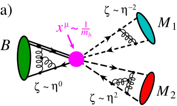
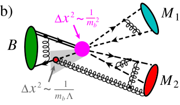
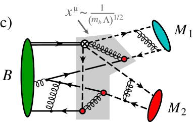
Figure -1139: Three types of factorization contributions to annihilation amplitudes which are the same order in $\eta=\Lambda_{\rm QCD}/m_{b}$. a) shows $Q_{i}^{(4)}$ which has $\geq 1$ hard gluon and factorizes at the scale $m_{b}$. The rapidity parameter, $\zeta=p^{-}/p^{+}$, controls the MS-factorization between soft momenta ($B$), $n$-collinear momenta ($M_{2}$), and ${\bar{n}}$-collinear momenta ($M_{1}$). b) shows the time-ordered product $Q_{i}^{(2)}{\cal L}^{(1)}_{\xi q}$, which involves factorization at $m_{b}$ and $\sqrt{m_{b}\Lambda}$. c) shows the time-ordered product $Q_{i}^{(1)}[{\cal L}^{(1)}_{\xi q}]^{3}$, which factorizes at the scale $\sqrt{m_{b}\Lambda}$ and does not need a hard gluon. Graphs a) and b) are of order $\alpha_{s}(\mu_{h})$, while c) is $\alpha_{s}(\mu_{i})^{2}$.

The annihilation amplitudes and other $\Lambda/m_{b}$ suppressed amplitudes also occur through time-ordered products. Two examples are shown by Figs. -1139b and -1139c. A subset of these terms were considered in Ref. Feldmann:2004mg , including the diagram in Fig. -1139c, and the phenomenological impact of these power corrections was studied. So far no attempt has been made to work out the strong phase properties and perturbative orders in $\alpha_{s}$ of the time-ordered products, a task we take up here. A complete classification of time-ordered products for the leading power corrections to $B\to M_{1}M_{2}$ is listed in Table 1. A subset of these terms contribute to the annihilation amplitudes. To see which, we note that terms with a $Q^{(0,1)}_{i}$ and only one ${\cal L}_{\xi q}^{(1)}$ do not contribute to annihilation at either leading or next-to-leading order; the weak operator is not high enough order in $\lambda$ to contain an extra $n$–${\bar{n}}$ pair, and there are not enough ${\cal L}_{\xi q}$’s to produce the pair through a soft quark exchange. To rule out these terms it was important that we are not considering isosinglet final states, which receive emission annihilation contributions already at leading order. The term $Q_{i}^{(2)}[{\cal L}_{\xi q}^{(1)}]^{2}$ does not contribute to annihilation because we find that all annihilation type contractions are further power suppressed when matched onto ${\rm SCET}_{\rm II}$.

Time-ordered products with either a $Q^{(j\geq 2)}$ or with three ${\cal L}_{\xi q}$’s do contribute to annihilation. Examples of these two types are shown in Figs. -1139b and -1139c. Compared to the local annihilation amplitude from $Q_{i}^{(4)}$, only the time-ordered product $Q^{(2)}{\cal L}_{\xi q}^{(1)}$ contributes at the same order in $\alpha_{s}$. To demonstrate this, note that for terms with three ${\cal L}_{\xi q}$’s all graphs have at least two contracted hard-collinear gluons and so are ${\cal O}(\alpha_{s}^{2}(\mu_{i}))$. Graphs with a $Q^{(2,3)}$ start with one $\alpha_{s}(\mu_{h})$, and will also have an additional $\alpha_{s}(\mu_{i})$ from a hard collinear gluon, unless it remains uncontracted in matching onto ${\rm SCET}_{\rm II}$. The uncontracted gluon costs an additional $\lambda$ in the matching onto ${\rm SCET}_{\rm II}$, so only the time-ordered product $Q^{(2)}{\cal L}_{\xi q}^{(1)}$ can have a leading, ${\cal O}(\alpha_{s}(m_{b}))$, contribution. Fig. -1139b gives an example of a diagram occurring from this time-ordered product. The resulting amplitude involves the three-parton distribution, $\phi_{3M_{2}}$. As shown in Ref. Arnesen2 it also involves the twist-2 distribution $\phi_{B}^{+}$, and its leading order convolution integrals converge.

The time-ordered products with three ${\cal L}_{\xi q}$’s are suppressed by $\alpha_{s}^{2}(\mu_{i})/\alpha_{s}(\mu_{h})$ relative to $Q^{(4)}_{i}$, and can be proven to involve a complex nonperturbative function, as labeled in Table 1 (an example is shown in Fig. -1139c). Thus, if perturbation theory converges rapidly at the scale $\mu_{i}$, then complex annihilation amplitudes are highly suppressed. If perturbation theory at $\mu_{i}$ is poorly convergent then the time-ordered product contribution could be important numerically; comparable or even larger than the leading local annihilation amplitude from $Q_{i}^{(4)}$. Local annihilation contributions are discussed in detail in sections III and IV, while strong phase properties of the amplitudes and the time-ordered product contributions are taken up in section V.

III Local six-quark operators in ${\rm SCET}_{\rm II}$

In this section we construct a complete basis of $O_{i}^{(1L)}$ operators in ${\rm SCET}_{\rm II}$ (the $Q_{i}^{(4)}$ terms in ${\rm SCET}_{\rm I}$) and derive a factorization theorem for their contributions to $B\to M_{1}M_{2}$. To find a complete basis we consider color, spin, and flavor structures that could appear when matching at any order in $\alpha_{s}$. Color is simple, the six-quark operator must have $\Gamma_{s}\otimes\Gamma_{\bar{n}}\otimes\Gamma_{n}=1\otimes 1\otimes 1$. Although operators with a $T^{A}$ in one or more bilinears are allowed at this order, with the factorization properties of the leading Lagrangians and $\langle M_{n}M_{\bar{n}}|O|B_{s}\rangle=\langle 0|\ldots|B_{s}\rangle\langle M_{\bar{n}}|\ldots|0\rangle\langle M_{n}|\ldots|0\rangle$, the terms with $T^{A}$’s give vanishing matrix element between the color singlet hadronic states Bauer:2001cu .

For spin we start by looking at chirality which is preserved by the matching at $m_{b}$. Since there is no jet function, the soft spectator quark that interpolates for the $B$-meson must come from the original operator in $H_{W}$, and we Fierz this $\bar{\psi}$ field next to the $b$-quark field. To be definite, we take the other $\bar{\psi}$ field from $H_{W}$ to go in the ${\bar{n}}$ direction (in the SCET Hamiltonian we sum over $n\leftrightarrow{\bar{n}}$). This implies that the pair-produced quark is in the $n$ direction. For $O_{1-4,9,10}$ the allowed chiral structures induced in SCET by matching are $(LH)(LL)(LL)$ and $(LH)(LR)(RL)$ where $L$ and $R$ correspond to the handedness for the light quarks in the bilinears in the order shown in Eq. (12). We cannot assign a handedness to the heavy quark denoted here by $H$. For $O_{5-8}$ we can have $(LH)(RL)(LR)$, $(LH)(RR)(RR)$, $(RH)(LL)(LR)$, and $(RH)(LR)(RR)$. A complete basis of Dirac structures for the individual bilinears is:

$$\Gamma_{s}=\gamma^{\alpha}\,,\qquad\Gamma_{\bar{n}}=\{\not{n},\not{n}\gamma_{\perp}^{\nu}\}\,,\qquad\Gamma_{n}=\{\not{\bar{n}},\not{\bar{n}}\gamma_{\perp}^{\mu}\}\,.$$ (13)

Structures with $\gamma_{5}$ are not needed because we have specified the handedness. Here $\not{\bar{n}}\gamma_{\perp}^{\mu}$ and $\not{n}\gamma_{\perp}^{\nu}$ connect left and right-handed quarks, while $\not{\bar{n}}$ and $\not{n}$ connect quarks of the same handedness. From the basis in Eq. (13) we must construct an overall scalar using the tensors $v^{\mu}$, $n^{\mu}$, ${\bar{n}}^{\mu}$, $g_{\perp}^{\mu\nu}$, and $\epsilon_{\perp}^{\mu\nu}\equiv\epsilon^{\mu\nu\alpha\beta}{\bar{n}}_{\alpha}n_{\beta}/2$. We take $\epsilon^{0123}=1$, and work in a frame where $v_{\perp}^{\mu}=0$ and $n\cdot v={\bar{n}}\cdot v=1$, which makes the set $\{n,{\bar{n}},v\}$ redundant. For reasons that will become apparent we pick $v^{\mu}$ and $(n^{\mu}-{\bar{n}}^{\mu})$ as our basis in this section. The definite handedness allows us to turn any contraction involving $i\epsilon_{\perp}^{\mu\nu}$ into a contraction with $g_{\perp}^{\mu\nu}$, for example $i\epsilon_{\perp}^{\mu\nu}\bar{\xi}_{n}^{L}\not{\bar{n}}\gamma^{\perp}_{\nu}\xi_{n}^{R}=\bar{\xi}_{n}^{L}\not{\bar{n}}\gamma_{\perp}^{\mu}\gamma_{5}\xi_{n}^{R}=\bar{\xi}_{n}^{L}\not{\bar{n}}\gamma_{\perp}^{\mu}\xi_{n}^{R}$. The $(LH)(LR)(RL)$ and $(LH)(RL)(LR)$ structures can be ruled out since

$$\not{n}\gamma_{\perp}^{\mu}P_{R}\otimes\not{\bar{n}}\gamma^{\perp}_{\mu}P_{L}=\not{n}\gamma_{\perp}^{\mu}P_{L}\otimes\not{\bar{n}}\gamma^{\perp}_{\mu}P_{R}=0\,.$$ (14)

Noting that $v\!\!\!/h_{v}=h_{v}$ this leaves four allowed spin structures

$$\Gamma_{s}\otimes\Gamma_{\bar{n}}\otimes\Gamma_{n}=\big{\{}1\otimes\not{n}\otimes\not{\bar{n}},\ (\not{\bar{n}}\!-\!\not{n})\otimes\not{n}\otimes\not{\bar{n}},\ \gamma_{\perp}^{\alpha}\otimes\not{n}\otimes\not{\bar{n}}\gamma^{\perp}_{\alpha},\ \gamma_{\perp}^{\alpha}\otimes\not{n}\gamma^{\perp}_{\alpha}\otimes\not{\bar{n}}\big{\}}\,.$$ (15)

The last two structures have $\bar{q}_{s}\gamma_{\perp}^{\alpha}b_{v}$ and vanish identically for $B$-meson decays (they would contribute for $B^{*}$’s). Furthermore, the local annihilation operators are not sensitive to the $k^{+}$ momentum of the soft spectator quark. Thus in taking the matrix element we can use

$$\langle 0|\bar{q}_{s}\gamma_{5}h_{v}|B\rangle=-im_{B}f_{B}\,,\qquad\langle 0|\bar{q}_{s}\gamma_{5}(\not{\bar{n}}\!-\!\not{n})h_{v}|B\rangle=0\,.$$ (16)

Here $f_{B}$ is the decay constant in the heavy quark limit. The fact that we can match onto a basis of local SCET operators of the form in Eq. (12) demonstrates to all orders in $\alpha_{s}$ that the local annihilation contributions are proportional to $f_{B}$. Using Eq. (16) the second Dirac structure in Eq. (15) is eliminated, so we do not list operators with $(\not{\bar{n}}\!-\!\not{n})$ in the soft bilinears below.

Next we consider the allowed flavor structures. From the operators $O_{1,2}$ we have $(\bar{u}b)(\bar{d}q)(\bar{q}u)$, $(\bar{d}b)(\bar{u}q)(\bar{q}u)$, from $O_{1-6,7\gamma,8g}$ we have $(\bar{d}b)(\bar{q}^{\prime}q)(\bar{q}q^{\prime})$, $(\bar{q}^{\prime}b)(\bar{d}q)(\bar{q}q^{\prime})$, and $O_{7-10}$ give a combination of these. Here the $q\bar{q}$ are the pair produced $n$ and ${\bar{n}}$ pair, while the $q^{\prime}\bar{q}^{\prime}$ appeared in the weak operators. Thus a basis for $B$-decay operators is

$$O_{1d}^{(1L)} = \frac{2}{m_{b}^{3}}\,{\textstyle\sum}_{q}\,\big{[}\bar{d}_{s}P_{R}{b}_{v}\big{]}\big{[}\bar{u}_{{\bar{n}},\omega_{2}}\not{n}P_{L}\,q_{{\bar{n}},\omega_{3}}\big{]}\big{[}\bar{q}_{n,\omega_{1}}\not{\bar{n}}P_{L}u_{n,\omega_{4}}\big{]}\,,$$

$$O_{2d}^{(1L)} = \frac{2}{m_{b}^{3}}\,{\textstyle\sum}_{q}\,\big{[}\bar{u}_{s}P_{R}{b}_{v}\big{]}\big{[}\bar{d}_{{\bar{n}},\omega_{2}}\not{n}P_{L}\,q_{{\bar{n}},\omega_{3}}\big{]}\big{[}\bar{q}_{n,\omega_{1}}\not{\bar{n}}P_{L}u_{n,\omega_{4}}\big{]}\,,$$

$$O_{3d}^{(1L)} = \frac{2}{m_{b}^{3}}\,{\textstyle\sum}_{q,q^{\prime}}\,\big{[}\bar{d}_{s}P_{R}{b}_{v}\big{]}\big{[}\bar{q}^{\prime}_{{\bar{n}},\omega_{2}}\not{n}P_{L}\,q_{{\bar{n}},\omega_{3}}\big{]}\big{[}\bar{q}_{n,\omega_{1}}\not{\bar{n}}P_{L}q^{\prime}_{n,\omega_{4}}\big{]}\,,$$

$$O_{4d}^{(1L)} = \frac{2}{m_{b}^{3}}\,{\textstyle\sum}_{q,q^{\prime}}\,\big{[}\bar{q}^{\prime}_{s}P_{R}{b}_{v}\big{]}\big{[}\bar{d}_{{\bar{n}},\omega_{2}}\not{n}P_{L}\,q_{{\bar{n}},\omega_{3}}\big{]}\big{[}\bar{q}_{n,\omega_{1}}\not{\bar{n}}P_{L}q^{\prime}_{n,\omega_{4}}\big{]}\,,$$

$$O_{5d}^{(1L)} = \frac{2}{m_{b}^{3}}\,{\textstyle\sum}_{q}\,\big{[}\bar{d}_{s}P_{R}{b}_{v}\big{]}\big{[}\bar{u}_{{\bar{n}},\omega_{2}}\not{n}P_{R}\,q_{{\bar{n}},\omega_{3}}\big{]}\big{[}\bar{q}_{n,\omega_{1}}\not{\bar{n}}P_{R}\,u_{n,\omega_{4}}\big{]}\,,$$

$$O_{6d}^{(1L)} = \frac{2}{m_{b}^{3}}\,{\textstyle\sum}_{q}\,\big{[}\bar{u}_{s}P_{R}{b}_{v}\big{]}\big{[}\bar{d}_{{\bar{n}},\omega_{2}}\not{n}P_{R}\,q_{{\bar{n}},\omega_{3}}\big{]}\big{[}\bar{q}_{n,\omega_{1}}\not{\bar{n}}P_{R}\,u_{n,\omega_{4}}\big{]}\,,$$

$$O_{7d}^{(1L)} = \frac{2}{m_{b}^{3}}\,{\textstyle\sum}_{q,q^{\prime}}\,\big{[}\bar{d}_{s}P_{R}{b}_{v}\big{]}\big{[}\bar{q}^{\prime}_{{\bar{n}},\omega_{2}}\not{n}P_{R}\,q_{{\bar{n}},\omega_{3}}\big{]}\big{[}\bar{q}_{n,\omega_{1}}\not{\bar{n}}P_{R}\,q^{\prime}_{n,\omega_{4}}\big{]}\,,$$

$$O_{8d}^{(1L)} = \frac{2}{m_{b}^{3}}\,{\textstyle\sum}_{q,q^{\prime}}\,\big{[}\bar{q}^{\prime}_{s}P_{R}{b}_{v}\big{]}\big{[}\bar{d}_{{\bar{n}},\omega_{2}}\not{n}P_{R}\,q_{{\bar{n}},\omega_{3}}\big{]}\big{[}\bar{q}_{n,\omega_{1}}\not{\bar{n}}P_{R}\,q^{\prime}_{n,\omega_{4}}\big{]}\,.$$ (17)

Here we integrated out $c$ and $b$ quarks in the sum over flavors, so the remaining sums are over $q=u,d,s$ and $q^{\prime}=u,d,s$. For the $\Delta S=0$ effective Hamiltonian with Wilson coefficients $a_{i}^{(d)}(\omega_{j})$ we use the notation

$$H_{W}=\frac{4G_{F}}{\sqrt{2}}\,\sum_{n,{\bar{n}}}\int[d\omega_{1}d\omega_{2}d\omega_{3}d\omega_{4}]\,\sum_{i=1-8}a_{i}^{d}(\omega_{j})\,O_{id}^{(1L)}(\omega_{j})\,.$$ (18)

To pull the CKM structures out of the SCET Wilson coefficients we write

$$a_{i}^{d}(\omega_{j})=\Bigg{\{}\begin{array}[]{lc}\lambda^{(d)}_{u}\,a_{iu}(\omega_{j})+\lambda^{(d)}_{c}\,a_{ic}(\omega_{j})&[i=1,2,3,4]\,,\\[4.0pt] (\lambda^{(d)}_{u}+\lambda^{(d)}_{c})\,a_{i}(\omega_{j})&[i=5,6,7,8]\,,\end{array}$$ (19)

where $\lambda_{p}^{(d)}=V_{pb}V^{*}_{pd}$. Identical definitions for $a_{i}^{s}$ are made by replacing $\lambda_{u}^{(d)}\to\lambda_{u}^{(s)}$ and $\lambda_{c}^{(d)}\to\lambda_{c}^{(s)}$. For $i=5,6,7,8$ only penguin operators contribute.

Next we take the $B\to M_{1}M_{2}$ matrix element of $H_{W}$. The factorization properties of SCET yield

$$\langle M_{1}M_{2}|O_{1d}^{(1L)}|B\rangle =\frac{2}{m_{b}^{3}}\,{\textstyle\sum}_{q}\,\langle M_{1}|\bar{u}_{{\bar{n}},\omega_{2}}\not{n}P_{L}\,q_{{\bar{n}},\omega_{3}}|0\rangle\langle M_{2}|\bar{q}_{n,\omega_{1}}\not{\bar{n}}P_{L}u_{n,\omega_{4}}|0\rangle\langle 0|\bar{d}_{s}P_{R}{b}_{v}|B\rangle$$

$$\quad+\big{\{}M_{1}\leftrightarrow M_{2}\big{\}}\,,$$ (20)

with similar results for the other $O_{id}^{(1L)}$ terms. Here the $\{M_{1}\leftrightarrow M_{2}\}$ indicates terms where the flavor quantum numbers of the $M_{2}$ state match those of the ${\bar{n}}$-collinear operator. The matrix elements in Eq. (III) are zero for transversely polarized vector mesons in agreement with the helicity counting in Ref. alex . Equation (III) can be evaluated using Eq. (16) and

$$\langle P_{n_{1}}(p)|\bar{q}^{(f)}_{n,\omega}\,\not{\bar{n}}P_{L,R}\,q^{(f^{\prime})}_{n,\omega^{\prime}}|0\rangle =\frac{\pm i\,f_{P}}{2}\,c_{Pff^{\prime}}\,\delta_{nn_{1}}\,\delta({\bar{n}}\!\cdot\!p\!-\!\omega\!+\!\omega^{\prime})\,\phi_{P}(y)\,,$$

$$\langle V_{n_{1}}(p,\varepsilon)|\bar{q}^{(f)}_{n,\omega}\,\not{\bar{n}}P_{L,R}\,q^{(f^{\prime})}_{n,\omega^{\prime}}|0\rangle =\frac{if_{V}m_{V}{{\bar{n}}\!\cdot\!\varepsilon}}{2\,{\bar{n}}\!\cdot\!p}\,c_{Vff^{\prime}}\,\delta_{nn_{1}}\,\delta({\bar{n}}\!\cdot\!p\!-\!\omega\!+\!\omega^{\prime})\,\phi_{V_{\parallel}}(y)\,.$$ (21)

Here $f,f^{\prime}$ are flavor indices, $\phi_{P}(y)$ and $\phi_{V_{\parallel}}(y)$ are the twist-2 light-cone distribution functions for pseudoscalars and vectors, $y=\omega/{\bar{n}}\cdot p=\omega/m_{b}$, and $c_{Pff^{\prime}}$, $c_{Vff^{\prime}}$ are Clebsch-Gordan coefficients. For the $M_{2}$ mesons, $P_{n_{2}}$ and $V_{n_{2}}$, we have the same equation with $n\leftrightarrow{\bar{n}}$, and $y\to x$. Since the $P_{L,R}$ only induce $\pm$ signs in the pseudoscalar matrix element, it is convenient to define

$M_{1}M_{2}$	$H(x,y)$
$\pi^{-}\pi^{+}$, $\pi^{-}\rho^{+}$, $\rho^{-}\pi^{+}$, $\rho^{-}\rho^{+}$	$-\tilde{a}^{d}_{1}(x,y)-\tilde{a}^{d}_{4}(y,x)-\tilde{a}^{d}_{3}(x,y)-\tilde{a}_{3}^{d}(y,x)$
$\pi^{-}\pi^{0}$, $\rho^{-}\pi^{0}$ $\pi^{-}\rho^{0}$, $\rho^{-}_{\parallel}\rho^{0}_{\parallel}$	$\frac{1}{\sqrt{2}}\big{[}\tilde{a}^{d}_{2}(x,y)+\tilde{a}^{d}_{4}(x,y)-\tilde{a}^{d}_{2}(y,x)-\tilde{a}^{d}_{4}(y,x)\big{]}$
$\pi^{0}\pi^{0},$ $\pi^{0}\rho^{0}$, $\rho^{0}\rho^{0}$	$\big{[}\frac{1}{2}\tilde{a}^{d}_{1}(x,y)+\tilde{a}^{d}_{3}(x,y)+\frac{1}{2}\tilde{a}^{d}_{4}(x,y)\big{]}+\big{[}x\leftrightarrow y\big{]}$
$K^{(*)-}K^{(*)+}$	$-\tilde{a}^{d}_{1}(x,y)-\tilde{a}^{d}_{3}(x,y)-\tilde{a}^{d}_{3}(y,x)$
$\bar{K}^{(*)0}K^{(*)0}$	$\tilde{a}^{d}_{3}(x,y)+\tilde{a}^{d}_{3}(y,x)+\tilde{a}^{d}_{4}(x,y)$
$K^{(*)-}K^{(*)0}$	$\tilde{a}^{d}_{2}(x,y)+\tilde{a}^{d}_{4}(x,y)$
$\pi^{-}\bar{K}^{(*)0}$, $\rho^{-}\bar{K}^{(*)0}$	$\tilde{a}_{2}^{s}(x,y)+\tilde{a}_{4}^{s}(x,y)$
$\pi^{0}\bar{K}^{(*)-},\rho^{0}{K}^{(*)-}$	$-\frac{1}{\sqrt{2}}\big{[}\tilde{a}_{2}^{s}(x,y)+\tilde{a}_{4}^{s}(x,y)\big{]}$
$\pi^{0}\bar{K}^{(*)0},\rho^{0}\bar{K}^{(*)0}$	$\frac{1}{\sqrt{2}}\,\tilde{a}_{4}^{s}(x,y)$
$\pi^{+}K^{(*)-},\rho^{+}K^{(*)-}$	$-\tilde{a}_{4}^{s}(x,y)$

Table 2: Hard functions for $\bar{B}^{0}$ and $B^{-}$ decays for the annihilation amplitude $A_{Lann}^{(1)}$ in Eq. (23). For each pair of mesons in the table, the first is $M_{1}$ and the second $M_{2}$.

$M_{1}M_{2}$	$H(x,y)$
$\pi^{-}K^{(*)+}$, $\rho^{-}K^{(*)+}$	$-\tilde{a}^{d}_{4}(y,x)$
$\pi^{0}K^{(*)0}$, $\rho^{0}K^{(*)0}$	$\frac{1}{\sqrt{2}}\,\tilde{a}^{d}_{4}(y,x)$
$\pi^{-}\pi^{+}$, $\pi^{-}\rho^{+}$, $\rho^{-}\pi^{+}$, $\rho^{-}\rho^{+}$	$-\tilde{a}^{s}_{1}(x,y)-\tilde{a}^{s}_{3}(x,y)-\tilde{a}_{3}^{s}(y,x)$
$\pi^{0}\pi^{0},$ $\pi^{0}\rho^{0}$, $\rho^{0}\rho^{0}$	$\big{[}\frac{1}{2}\tilde{a}^{s}_{1}(x,y)+\tilde{a}^{s}_{3}(x,y)\big{]}+\big{[}x\leftrightarrow y\big{]}$
$K^{(*)-}K^{(*)+}$	$-\tilde{a}^{s}_{1}(x,y)-\tilde{a}^{s}_{4}(y,x)-\tilde{a}^{s}_{3}(x,y)-\tilde{a}_{3}^{s}(y,x)$
$\bar{K}^{(*)0}K^{(*)0}$	$\tilde{a}^{s}_{3}(x,y)+\tilde{a}^{s}_{3}(y,x)+\tilde{a}^{s}_{4}(y,x)$

Table 3: Hard functions for $\bar{B}_{s}$ decays for the annihilation amplitude $A_{Lann}^{(1)}$ in Eq. (23).

$$\tilde{a}_{1}^{d}=a_{1}^{d}+\kappa a_{5}^{d}\,,\qquad\tilde{a}_{2}^{d}=a_{2}^{d}+\kappa a_{6}^{d}\,,\qquad\tilde{a}_{3}^{d}=a_{3}^{d}+\kappa a_{7}^{d}\,,\qquad\tilde{a}_{4}^{d}=a_{4}^{d}+\kappa a_{8}^{d}\,,$$ (22)

with similar definitions for $\tilde{a}_{i}^{s}$. Here $\kappa=+1$ for $PP$, $VV$, and $\kappa=-1$ for $PV$ channels. Using these results, the ${\cal O}(\Lambda/m_{b})$ local annihilation amplitudes are

$$A^{(1)}_{Lann}(\bar{B}\to M_{1}M_{2})=-\frac{G_{F}f_{B}f_{M_{1}}f_{M_{2}}}{\sqrt{2}}\int_{0}^{1}\!\!dx\,dy\,H(x,y)\,\phi^{M_{1}}(y)\phi^{M_{2}}(x)\,.$$ (23)

Here $H(x,y)$ are perturbatively calculable hard coefficients determined by the SCET Wilson coefficients $\tilde{a}_{i}(\omega_{j})$. Results for different final states are listed in Table 2 for $\bar{B}^{0}$ and $B^{-}$ decays, and in Table 3 for $\bar{B}_{s}$ decays. Our derivation of the local annihilation amplitude in Eq. (23) is valid to all orders in $\alpha_{s}$, and provides a proof of factorization for this term.

Matching at tree level, involves computing the ${\cal O}(\alpha_{s}(m_{b}))$ graphs in Fig. -1138 and comparing them with matrix elements of the SCET operators $Q_{i}^{(4)}$. Doing so we find that the Wilson coefficients $a_{i}(x,y)$ are

$$a_{1u} =\frac{C_{F}\pi\alpha_{s}(\mu_{h})}{N_{c}^{2}}\,F(x,y)\,\Big{(}C_{1}+\frac{3}{2}\,C_{10}\Big{)}\,, a_{1c} =\frac{C_{F}\pi\alpha_{s}(\mu_{h})}{N_{c}^{2}}\,F(x,y)\,\Big{(}\frac{3}{2}\,C_{10}\Big{)}\,,$$

$$a_{2u} =\frac{C_{F}\pi\alpha_{s}(\mu_{h})}{N_{c}^{2}}\,F(x,y)\,\Big{(}C_{2}+\frac{3}{2}\,C_{9}\Big{)}\,, a_{2c} =\frac{C_{F}\pi\alpha_{s}(\mu_{h})}{N_{c}^{2}}\,F(x,y)\,\Big{(}\frac{3}{2}\,C_{9}\Big{)}\,,$$

$$a_{3u} =\frac{C_{F}\pi\alpha_{s}(\mu_{h})}{N_{c}^{2}}\,F(x,y)\,\Big{(}C_{4}-\frac{1}{2}\,C_{10}\Big{)}\,, a_{3c} =\frac{C_{F}\pi\alpha_{s}(\mu_{h})}{N_{c}^{2}}\,F(x,y)\,\Big{(}C_{4}-\frac{1}{2}\,C_{10}\Big{)}\,,$$

$$a_{4u} =\frac{C_{F}\pi\alpha_{s}(\mu_{h})}{N_{c}^{2}}\,F(x,y)\,\Big{(}C_{3}-\frac{1}{2}\,C_{9}\Big{)}\,, a_{4c} =\frac{C_{F}\pi\alpha_{s}(\mu_{h})}{N_{c}^{2}}\,F(x,y)\,\Big{(}C_{3}-\frac{1}{2}\,C_{9}\Big{)}\,,$$

$$a_{5} =\frac{C_{F}\pi\alpha_{s}(\mu_{h})}{N_{c}^{2}}\,F(\bar{y},\bar{x})\Big{(}\frac{3}{2}\,C_{8}\Big{)}\,, a_{6} =0\,,$$

$$a_{7} =\frac{C_{F}\pi\alpha_{s}(\mu_{h})}{N_{c}^{2}}\,F(\bar{y},\bar{x})\Big{(}C_{6}-\frac{1}{2}\,C_{8}\Big{)}\,, a_{8} =0\,,$$ (24)

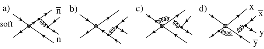
Figure -1138: Tree level annihilation graphs for $B\to M_{1}M_{2}$ decays. Here soft, $n$, ${\bar{n}}$ denote quarks that are soft, $n$-collinear, and ${\bar{n}}$-collinear respectively.

where $\mu_{h}\sim m_{b}$, $\bar{x}=1-x$, $\bar{y}=1-y$, with quark momentum fractions $x$ and $y$ as defined in Eq. (III) and shown in Fig. -1138. The function $F$ is

$$F(x,y)=\bigg{[}\frac{1}{\bar{x}^{2}y}-\frac{1}{y(x\bar{y}-1)}\bigg{]}_{\mbox{\o}}\ +\frac{d(\mu_{-})\>\delta^{\prime}(\bar{x})}{y}\,,$$ (25)

where the ø-notation and term involving the Wilson coefficient $d(\mu_{-})$ are discussed below. The function $F(\bar{y},\bar{x})$ will involve $d(\mu_{+})$. Note that the coefficients $a_{3u,3c,4u,4c,7,8}$ are polluted in the sense of Ref. Bauer:2004tj , meaning that ${\cal O}(\alpha_{s}^{2})$ matching results proportional to the large coefficients $C_{1,2}$ could compete numerically. The others are not polluted: $a_{1u,2u}$ involve $C_{1,2}$ at ${\cal O}(\alpha_{s})$, while $a_{1c,2c,5,6}$ only get contributions from electroweak penguins. Our results for the diagrams in Fig. -1138 agree with Refs. Keum ; BBNS2 . This includes the appearance of the combinations of momentum fractions in the functions $F(x,y)$ and $F(\bar{y},\bar{x})$, up to ø-distribution and $d$-term. For later convenience we define moment parameters which convolute the hard coefficients with the meson distributions

$$\beta_{iu}^{M_{1}M_{2}} =\int_{0}^{1}\!\!dx\,dy\,[a_{iu}(x,y)\!+\!\kappa a_{i+4}(x,y)]\,\phi^{M_{1}}(y)\phi^{M_{2}}(x)\,,$$

$$\beta_{ic}^{M_{1}M_{2}} =\int_{0}^{1}\!\!dx\,dy\,[a_{ic}(x,y)\!+\!\kappa a_{i+4}(x,y)]\,\phi^{M_{1}}(y)\phi^{M_{2}}(x)\,.$$ (26)

In Eq. (25) the subscript ø denotes the fact that singular terms in convolution integrals are finite in SCET due to the MS-factorization which involves convolution integrals such as

$$\sum_{x,\,x^{\prime}\neq 0}\int\!dx_{r}\,dx^{\prime}_{r}\,\delta(1\!-\!x\!-\!x^{\prime})\,\frac{\phi_{M}(x,x^{\prime},\mu)}{\bar{x}^{2}}\,,$$ (27)

where $x^{(\prime)}$ and $x^{(\prime)}_{r}$ correspond to label and residual momenta Manohar:2006nz . Implementing $x\neq 0$ and $x^{\prime}\neq 0$ in the MS-factorization scheme requires zero-bin subtractions and divergences in the rapidity must also be regulated. The $\delta$-function sets $x^{\prime}=1-x$, so $x^{\prime}\neq 0$ enforces $x\neq 1$. With the usual assumption that $\phi_{M}(x)$ vanishes at its endpoints with a power-like fall-off slower than quadratic, only integrals over $1/\bar{x}^{2}$ in $F(x,y)$ and $1/y^{2}$ in $F(\bar{y},\bar{x})$ require special care,

$$\big{\langle}\bar{x}^{-2}\big{\rangle}^{M}=\!\int_{0}^{1}\!\!\!dx\,\frac{\phi_{M}(x,\mu)}{(\bar{x}^{2})_{\mbox{\o}}}\,, \big{\langle}y^{-2}\big{\rangle}^{M} =\!\int_{0}^{1}\!\!\!dy\,\frac{\phi_{M}(x,\mu)}{(y^{2})_{\mbox{\o}}}\,.$$ (28)

The resulting moments $\langle\bar{x}^{-2}\rangle^{M}$ and $\langle y^{-2}\rangle^{M}$ should be considered hadronic parameters, for which we use the minimal subtraction scheme. Their value depends on $\mu$ and $\mu_{\pm}$ and are scheme dependent beyond the usual $\overline{\rm MS}$ scheme for $\phi_{M}$. This can be viewed as a modification of the distribution function, $\phi_{M}(x,\mu)\to\phi_{M}(x,\mu,\mu_{-})$, where the $x^{-2}$ moment of $\phi_{M}(x,\mu,\mu_{-})$ converges. In order to derive a result that makes it easy to find a model for these moments we follow Ref. Manohar:2006nz and assume there is no interference between the rapidity renormalization and invariant mass renormalization, which gives

$$\big{\langle}\bar{x}^{-2}\big{\rangle}^{M}=\!\int_{0}^{1}\!\!\!dx\,\frac{\phi_{M}(x,\mu)+\bar{x}\phi^{\prime}_{M}(1,\mu)}{\bar{x}^{2}}-\phi^{\prime}_{M}(1,\mu)\,\ln\Big{(}\frac{{\bar{n}}\!\cdot\!p_{M}}{\mu_{-}}\Big{)}\,,$$

$$\big{\langle}y^{-2}\big{\rangle}^{M}=\!\int_{0}^{1}\!\!\!dy\,\frac{\phi_{M}(y,\mu)-y\phi^{\prime}_{M}(0,\mu)}{y^{2}}+\phi^{\prime}_{M}(0,\mu)\,\ln\Big{(}\frac{n\!\cdot\!p_{M}}{\mu_{+}}\Big{)}\,.$$ (29)

Here $\phi_{M}^{\prime}(1)$ is generated by a zero-bin subtraction which avoids double counting the region where $\bar{x}\to 0$. When $\bar{x}\to 0$ the corresponding outgoing quark becomes soft, and this contribution is taken into account by a time-ordered product term in Table 1. To obtain the renormalized $\langle\bar{x}^{-2}\rangle^{M}$ result in Eq. (III) requires $1/\epsilon_{\rm UV}$ counterterms which correspond to operators with the ${\bar{n}}$-collinear bilinears in Eq. (III), $[\bar{u}_{{\bar{n}},\omega_{2}}\not{n}\gamma_{5}q_{{\bar{n}},\omega_{3}}]$ etc., which can be written as Manohar:2006nz

$$O_{ct} =\frac{\partial}{\partial\omega_{3}}(\bar{\xi}_{\bar{n}}W)_{\omega_{2}}\not{n}\gamma_{5}(W^{\dagger}\xi_{\bar{n}})_{\omega_{3}}\bigg{|}_{\omega_{3}\to 0}\,.$$ (30)

The matrix element of these terms is taken prior to performing the partial derivative and the limit $\omega_{3}\to 0$, and gives $\phi_{M}^{\prime}(1,\mu)$. These terms do not have a $\omega_{3}\neq 0$ restriction, and consistency of the renormalization procedure used to obtain Eq. (III) demands that the fields here are ${\bar{n}}$-collinear. An analogous set of terms are required for $\phi_{M}^{\prime}(0,\mu)$. These terms are real at any scale, which follows from the requirements discussed in section V for an ${\rm SCET}_{\rm II}$ operator to be able to generate a physical strong phase. The dependences on $\mu_{\pm}$ in Eq. (III) are canceled by the leading dependences on these scales, $d(\mu_{-})=\ln(p_{M}^{-}/\mu_{-})+\kappa$ and $d(\mu_{+})=\ln(p_{M}^{+}/\mu_{+})+\kappa$, which appeared in Eq. (25). Here $\kappa$ can be fixed by a matching computation. The $d(\mu_{\pm})$ correspond to the renormalized coefficients of the $O_{ct}$, and must be included for consistency at this order LMS . In the rough numerical analysis we do later on, we will treat the contributions from these coefficients as part of the uncertainty.

Note that in deriving the result in Eq. (25) we have dropped $i\epsilon$ factors from the propagators. If these terms were kept, the second term in $F(x,y)$ would be

$$\frac{1}{(y+i\epsilon)\,(x\bar{y}-1+i\epsilon)}\,.$$ (31)

The $i\epsilon$’s yield imaginary contributions with $\delta(y)$ and $\delta(x\bar{y}-1)$. They contribute for $y=0$ or for $x=\bar{y}=1$, so these contributions occur in zero-bins, which are excluded from the convolution integrals in the factorization theorem we have derived with SCET. The zero-bins correspond to degrees of freedom that are soft, and including these regions would induce a double counting, so the correct factorization theorem in QCD does not include them. Factors analogous to $x\neq 0$ and $x^{\prime}\neq 0$ in Eq. (27) ensure that there is no contribution to the integral from any zero-bin momentum, and we find that the $\delta$-function terms give zero. This remains true for more singular distributions yielding $\delta^{(n)}(x)$, and so also applies to the first term in $F(x,y)$. Thus it is correct to drop the $i\epsilon$ factors from the start. This should be compared with the approach in KLS where the $i\epsilon$ factors generate a strong phase from the tree level diagrams from a $k_{\perp}^{2}$ dependent $\delta$-function. In our derivation any such $k_{\perp}^{2}$ imaginary terms could only occur at higher orders in $\Lambda/m_{b}$.

Thus at order $\alpha_{s}(\mu_{h})$ the lowest order annihilation factorization theorem is determined by the convolutions

$$\int_{0}^{1}\!dx\,dy\,F(x,y)\phi^{M_{1}}(y)\phi^{M_{2}}(x)$$ (32)

$$\qquad=\big{\langle}\bar{x}^{-2}\big{\rangle}^{M_{2}}\big{\langle}y^{-1}\big{\rangle}^{M_{1}}-\big{\langle}[y(x\bar{y}-1)]^{-1}\big{\rangle}^{M_{1}M_{2}}+d(\mu_{-})\phi_{M_{2}}^{\prime}(1)\big{\langle}y^{-1}\big{\rangle}^{M_{1}}\,,$$

$$\int_{0}^{1}\!dx\,dy\,F(\bar{y},\bar{x})\phi^{M_{1}}(y)\phi^{M_{2}}(x)$$

$$\qquad=\big{\langle}y^{-2}\big{\rangle}^{M_{1}}\big{\langle}\bar{x}^{-1}\big{\rangle}^{M_{2}}-\big{\langle}[\bar{x}(x\bar{y}-1)]^{-1}\big{\rangle}^{M_{1}M_{2}}-d(\mu_{+})\phi_{M_{1}}^{\prime}(0)\big{\langle}\bar{x}^{-1}\big{\rangle}^{M_{2}}\,.$$

Here we use Eq. (III), and

$$\langle y^{-1}\rangle^{M} =\int_{0}^{1}\!\!dy\,\frac{\phi^{M}(y,\mu)}{y}\,, \langle f(x,y)\rangle^{M_{1}M_{2}} =\int_{0}^{1}\!\!dx\!\int_{0}^{1}\!\!dy\,f(x,y)\,\phi^{M_{1}}(y,\mu)\,\phi^{M_{2}}(x,\mu).$$ (33)

These results do not have a complex phase because the right-hand side of Eq. (32) is real.

We have shown that the convolution formula in Eq. (23) for the local contributions $O_{i}^{(1L)}$ yields a well-defined annihilation amplitude. At order $\alpha_{s}(m_{b})$ the result is real, so $A^{(1)}_{Lann}$ is real up to perturbative corrections. Order $\alpha_{s}^{2}(m_{b})$ corrections to the $a_{i}$ will produce perturbative strong phases in $A^{(1)}_{Lann}$. Further discussion on strong phases is given in section V, while phenomenological implications are taken up in section VI.

IV Chirally Enhanced Local Annihilation Contributions

At order $\alpha_{s}(\mu_{h})\mu_{M}\Lambda/m_{b}^{2}$ there are contributions from chirally enhanced operators that could compete with the $\alpha_{s}(\mu_{h})\Lambda/m_{b}$ terms BBNS2 . In SCET we define these contributions as the set of ${\rm SCET}_{\rm II}$ operators analogous to $O^{(1L)}_{i}$ but with an extra $/\!\!\!\!{\cal P}_{\perp}$ between collinear quarks fields. We start by constructing a complete basis for local operators at this order with a ${\cal P}_{\perp}^{\beta}$, calling them $O^{(2L)}_{i}$. These operators have the same color and flavor structures as Eq. (III). The chiral structures induced from the operators $O_{1-10}$ and the initial basis of Dirac structures shown in Eq. (13) are also the same, and allow us to eliminate many possibilities.

The complete set of Dirac structures from matching the operators $O_{1-4,9,10}$ include

$$\Gamma_{s}\otimes\Gamma_{\bar{n}}\otimes\Gamma_{n}{\cal P}^{\beta}_{\perp}=\big{\{} \gamma^{\perp}_{\beta}\otimes\not{n}\otimes\not{\bar{n}}{\cal P}^{\beta}_{\perp},\ \gamma_{\perp}^{\alpha}\otimes\not{n}\gamma^{\perp}_{\alpha}\otimes\not{\bar{n}}\gamma^{\perp}_{\beta}{\cal P}^{\beta}_{\perp},\$$

$$\gamma^{\perp}_{\beta}\otimes\not{n}\gamma_{\perp}^{\alpha}\otimes\not{\bar{n}}\gamma^{\perp}_{\alpha}{\cal P}^{\beta}_{\perp},\ \gamma_{\perp}^{\alpha}\otimes\not{n}\gamma^{\perp}_{\beta}\otimes\not{\bar{n}}\gamma^{\perp}_{\alpha}{\cal P}^{\beta}_{\perp}\big{\}}\,,$$ (34)

plus the analogous set $\Gamma_{s}\otimes\Gamma_{\bar{n}}{\cal P}^{\beta}_{\perp}\otimes\Gamma_{n}$. Our basis does not include operators with ${\cal P}^{\dagger}_{\perp}$, because the mesons $M_{i}$ have zero $\perp$-momenta, so we can integrate these terms by parts to put them in the form in Eq. (IV). The third term in Eq. (IV) has chiral structure $(LH)(LR)(RL)$ and vanishes by Eq. (14). The terms in Eq. (IV) all have $\bar{q}_{s}\gamma_{\perp}^{\mu}b_{v}$, and so do not contribute for $B$-decays. The same holds if we replace ${\cal P}_{\perp}^{\beta}$ by $ig{\cal B}_{\perp}^{\beta}$. Thus, at any order in perturbation theory the only ${\cal O}(\eta^{8})$ local operator contributions from $O_{1-4,9,10}$ are those with a $D_{s}^{\mu}$ in the soft bilinear.

For $O_{5-8}$ we have the structures in Eq. (IV), and when the $q^{\prime}$ flavor is a soft quark with $P_{L}\otimes P_{R}$ Dirac structure from $O_{i}$ we also have

$$\Gamma_{s}\otimes\Gamma_{\bar{n}}\otimes\Gamma_{n}{\cal P}^{\beta}_{\perp}=\big{\{}1\otimes\not{n}\otimes\not{\bar{n}}\>/\!\!\!\!{\cal P}_{\perp},\ 1\otimes\not{n}\gamma^{\perp}_{\beta}\otimes\not{\bar{n}}{\cal P}_{\perp}^{\beta}\big{\}}\,,$$

$$\Gamma_{s}\otimes\Gamma_{\bar{n}}{\cal P}^{\beta}_{\perp}\otimes\Gamma_{n}=\big{\{}1\otimes\not{n}{\cal P}_{\perp}^{\beta}\otimes\not{\bar{n}}\gamma^{\perp}_{\beta},\ 1\otimes\not{n}\>/\!\!\!\!{\cal P}_{\perp}\otimes\not{\bar{n}}\,\big{\}}\,,$$ (35)

plus operators with 1 replaced by $\not{\bar{n}}-\not{n}$, which vanish due to Eq. (16). The operators in Eq. (IV) contribute to $B$-decays. In particular, they yield both transverse and longitudinal polarization in $B\to VV$. A complete basis for the local ${\cal O}(\eta^{8})$ operators with one ${\cal P}_{\perp}^{\beta}$ is

$$O_{1d}^{(2L)} =\frac{1}{m_{b}^{4}}\,{\textstyle\sum}_{q,q^{\prime}}\,\big{[}\bar{q}^{\prime}_{s}P_{L}{b}_{v}\big{]}\big{[}\bar{d}_{{\bar{n}},\omega_{2}}\not{n}P_{L}\,q_{{\bar{n}},\omega_{3}}\big{]}\big{[}\bar{q}_{n,\omega_{1}}\not{\bar{n}}\>/\!\!\!\!{\cal P}_{\perp}\!P_{R}\,q^{\prime}_{n,\omega_{4}}\big{]}\,,$$

$$O_{2d}^{(2L)} =\frac{1}{m_{b}^{4}}\,{\textstyle\sum}_{q,q^{\prime}}\,\big{[}\bar{q}^{\prime}_{s}P_{L}{b}_{v}\big{]}\big{[}\bar{d}_{{\bar{n}},\omega_{2}}\not{n}\>/\!\!\!\!{\cal P}_{\perp}\!P_{R}\,q_{{\bar{n}},\omega_{3}}\big{]}\big{[}\bar{q}_{n,\omega_{1}}\not{\bar{n}}P_{R}\,q^{\prime}_{n,\omega_{4}}\big{]}\,,$$

$$O_{3d}^{(2L)} =\frac{1}{m_{b}^{4}}\,{\textstyle\sum}_{q,q^{\prime}}\,\big{[}\bar{q}^{\prime}_{s}P_{L}{b}_{v}\big{]}\big{[}\bar{d}_{{\bar{n}},\omega_{2}}\not{n}\gamma^{\perp}_{\beta}P_{R}\,q_{{\bar{n}},\omega_{3}}\big{]}\big{[}\bar{q}_{n,\omega_{1}}\not{\bar{n}}P_{R}\,{\cal P}^{\beta}_{\perp}q^{\prime}_{n,\omega_{4}}\big{]}\,,$$

$$O_{4d}^{(2L)} =\frac{1}{m_{b}^{4}}\,{\textstyle\sum}_{q,q^{\prime}}\,\big{[}\bar{q}^{\prime}_{s}P_{L}{b}_{v}\big{]}\big{[}\bar{d}_{{\bar{n}},\omega_{2}}\not{n}P_{L}\,{\cal P}^{\beta}_{\perp}q_{{\bar{n}},\omega_{3}}\big{]}\big{[}\bar{q}_{n,\omega_{1}}\not{\bar{n}}\gamma^{\perp}_{\beta}P_{R}\,q^{\prime}_{n,\omega_{4}}\big{]}\,,$$

$$O_{5d-8d}^{(2L)} =O_{1d-4d}^{(2L)}\,\,\frac{3e_{q^{\prime}}}{2}\,,$$ (36)

with sums over $q,q^{\prime}=u,d,s$. Note that the flavor structure of these operators is identical to $O_{4d}^{(1L)}$. For the the electroweak penguin operators $O_{7,8}$ an additional four operators $O_{5d-8d}^{(2L)}$ are needed, which have the same spin-flavor structures as $O_{1d-4d}^{(2L)}$, but with an $e_{q^{\prime}}$ charge factor, $\sum_{q,q^{\prime}}3e_{q^{\prime}}/2$. Again we caution that we have not considered the complete set of local $\Lambda^{2}/m_{b}^{2}$ operators, since our basis does not include three-body terms with an $ig{\cal B}_{\perp}^{\mu}$, nor terms with an extra $D_{s}$ soft covariant derivative. We have also not considered ${\cal O}(\mu_{M_{1}}\mu_{M_{2}}\Lambda/m_{b}^{3})$ terms. All these terms are real, and it would be interesting to calculate them in the future.

The weak Hamiltonian with Wilson coefficients for the operators $O_{id}^{(2L)}$ is

$$H_{W}=\frac{4G_{F}}{\sqrt{2}}\,(\lambda^{(d)}_{u}+\lambda^{(d)}_{c})\sum_{n,{\bar{n}}}\int[d\omega_{1}d\omega_{2}d\omega_{3}d\omega_{4}]\,\sum_{i=1-8}a_{i}^{\chi}(\omega_{j})\,O_{id}^{(2L)}(\omega_{j})\,.$$ (37)

Since only the penguin operators $O_{5-8}$ contribute, we pulled out the common CKM factor. Matching at tree level onto the operators $O_{id}^{(2L)}$ by keeping terms linear in the $\perp$-momenta in Fig. -1138, we find

$$a^{\chi}_{1}(x,y) =\frac{4C_{F}\pi\alpha_{s}(\mu_{h})}{N_{c}}\,\bigg{[}\Big{(}C_{6}+\frac{C_{5}}{N_{c}}\Big{)}F_{1}(x,y)+\frac{C_{5}}{N_{c}}\,F_{2}(x,y)\bigg{]}_{\mbox{\o}}\,,$$

$$a^{\chi}_{2}(x,y) =\frac{4C_{F}\pi\alpha_{s}(\mu_{h})}{N_{c}}\,\bigg{[}-\Big{(}C_{6}+\frac{C_{5}}{N_{c}}\Big{)}F_{1}(\bar{y},\bar{x})+\frac{C_{5}}{N_{c}}\,F_{2}(\bar{y},\bar{x})\bigg{]}_{\mbox{\o}}\,,$$

$$a^{\chi}_{3}(x,y) =\frac{4C_{F}\pi\alpha_{s}(\mu_{h})}{N_{c}}\,\bigg{[}-\Big{(}C_{6}+\frac{C_{5}}{N_{c}}\Big{)}F_{3}(x,y)-\frac{C_{5}}{N_{c}}\,F_{2}(x,y)\bigg{]}_{\mbox{\o}}\,,$$

$$a^{\chi}_{4}(x,y) =\frac{4C_{F}\pi\alpha_{s}(\mu_{h})}{N_{c}}\,\bigg{[}\Big{(}C_{6}+\frac{C_{5}}{N_{c}}\Big{)}F_{3}(x,y)-\frac{C_{5}}{N_{c}}\,F_{2}(\bar{y},\bar{x})\bigg{]}_{\mbox{\o}}\,,$$

$$a^{\chi}_{5-8}(x,y) =a^{\chi}_{1-4}(x,y)\quad\mbox{with }C_{5}\to C_{7},\ C_{6}\to C_{8}\,,$$ (38)

where $x$ and $y$ are defined in Fig. -1138 and

$$F_{1}(x,y) =\bigg{[}\frac{1+\bar{x}}{y^{2}\,\bar{y}\,\bar{x}^{2}}\bigg{]}_{\mbox{\o}}\!\!+d_{1}(\mu_{-})\delta^{\prime}(\bar{x})\bigg{[}\frac{1}{y^{2}\bar{y}}\bigg{]}_{\mbox{\o}}\!\!+d_{2}(\mu_{+})\delta^{\prime}(y)\bigg{[}\frac{1+\bar{x}}{\bar{x}^{2}}\bigg{]}_{\mbox{\o}}\!\!+d_{3}(\mu_{\pm})\delta^{\prime}(\bar{x})\delta^{\prime}(y)\,,$$

$$F_{2}(x,y) =\bigg{[}\frac{1}{(1-x\bar{y})\bar{x}y^{2}}\bigg{]}_{\mbox{\o}}\,,$$

$$F_{3}(x,y) =\bigg{[}\frac{1}{y^{2}\,\bar{x}^{2}}\bigg{]}_{\mbox{\o}}\!\!+d_{4}(\mu_{-})\delta^{\prime}(\bar{x})\bigg{[}\frac{1}{y^{2}}\bigg{]}_{\mbox{\o}}\!\!+d_{5}(\mu_{+})\delta^{\prime}(y)\bigg{[}\frac{1}{\bar{x}^{2}}\bigg{]}_{\mbox{\o}}\!\!+d_{6}(\mu_{\pm})\delta^{\prime}(\bar{x})\delta^{\prime}(y)\,.$$ (39)

Here $d_{1-6}$ play the same role as $d$ in Eq. (25). The coefficients $a^{\chi}_{1-8}$ are polluted in the sense of Ref. Bauer:2004tj , meaning that ${\cal O}(\alpha_{s}^{2})$ matching results proportional to the large coefficients $C_{1,2}$ could compete numerically. This makes the computation of these ${\cal O}(\alpha_{s}^{2})$ corrections important.

For decays involving a pseudoscalar in the final state, the operators $O_{1d}^{(2L)}$ and $O_{2d}^{(2L)}$ generate so-called “chirally enhanced” terms, proportional to $\mu_{M}$. Time-ordered products of ${\rm SCET}_{\rm I}$ operators also generate $\mu_{M}$ terms, but only at ${\cal O}(\alpha_{s}^{2})$. It is not clear that the chirally enhanced terms are larger numerically than other power corrections. In particular three-body distributions from operators with $\bar{\xi}_{n}(ig{\cal B}_{\perp}^{\mu})\Gamma\xi_{n}$ are parametrically (and sometimes numerically as well) of similar importance Chernyak:1983ej . The distributions are related by Hardmeier:2003ig

$$f_{P}\mu_{P}\bigg{[}\phi^{P\,\prime}_{\sigma}(x)+\frac{(2x-1)}{x(1-x)}\,\phi_{\sigma}^{P}(x)\bigg{]} =-{6f_{3P}}\bigg{[}\frac{G_{P_{z}}^{(t)}(x)}{x}+\frac{G_{P_{y}}^{(t)}(x)}{1-x}\bigg{]}\,,$$

$$f_{P}\mu_{P}\bigg{[}\phi^{P}_{p}(x)-\frac{1}{6x(1-x)}\,\phi^{P}_{\sigma}(x)\bigg{]} =-{f_{3P}}\bigg{[}\frac{G_{P_{z}}^{(t)}(x)}{x}-\frac{G_{P_{y}}^{(t)}(x)}{1-x}\bigg{]}\,,$$ (40)

where $G_{P_{z}}^{(t)}(x)$ and $G_{P_{y}}^{(t)}(x)$ are integrals over the three-parton distribution, $\phi_{3P}$. These relations allow certain chirally enhanced terms with $\mu_{P}f_{P}$ to be traded for non-chirally enhanced terms with $f_{3P}$. Thus it is clear that the chirally enhanced terms dominate over the three-body operators only in the special case when the linear combinations in the square brackets on the left-hand side of Eq. (IV) are numerically suppressed. Solving with these linear combinations set to zero determines the two-body distributions $\phi_{\sigma}^{P}$ and $\phi_{p}^{P}$ in the Wandzura-Wilczek (WW) approximation Wandzura:1977qf . Thus in order to uniquely specify the $\mu_{P}$ dependent terms, the WW approximation was needed in Ref. BBNS2 .

In contrast, in SCET we are not forced to assume a numerical dominance of the $\mu_{P}$ terms to uniquely identify them. We can instead define local chirally enhanced annihilation terms to be the matrix elements of the operators $O_{1d}^{(2L)}$ and $O_{2d}^{(2L)}$ for final states with a pseudoscalar. With a minimal basis of operators, the matrix elements of these terms are unique. The remaining terms involve other operators, and we postpone discussing them to future work. We proceed to work out the factorization formula for $O_{1d}^{(2L)}$ and $O_{2d}^{(2L)}$ with steps analogous to Eqs. (III) through (23). To take the matrix element we need Eq. (III) and the result

$$\langle P_{n_{1}}(p)|\,\bar{q}^{(f)}_{n,\omega}\,\not{\bar{n}}\,\,{/\!\!\!\!{\cal P}_{\perp}}P_{R}\,q^{(f^{\prime})}_{n,\omega^{\prime}}\,|0\rangle=-\frac{i}{6}\,c_{Pff^{\prime}}\,\delta_{nn_{1}}\,\delta({\bar{n}}\!\cdot\!p-\omega+\omega^{\prime})\,f_{P}\mu_{P}\,\phi_{pp}^{P}(y)\,.$$ (41)

Here $c_{Pff^{\prime}}$ are Clebsch-Gordan factors, $y=\omega/{\bar{n}}\cdot p$, and we have not written the $\omega^{\prime}$ dependence in the distribution due to the $\delta$-function. The distribution $\phi^{P}_{pp}(y)$ is related to more standard twist-3 two-parton and three-parton distributions by Hardmeier:2003ig ; Manohar:2006nz

$$\phi^{P}_{pp}(y)={3y}\bigg{[}\phi^{P}_{p}(y)+\frac{1}{6}\,\phi^{P\prime}_{\sigma}(y)+\frac{2\,f_{3P}}{f_{P}\mu_{P}}\,\int\frac{dy^{\prime}}{y^{\prime}}\,\phi_{3P}(y-y^{\prime},y)\bigg{]}\,.$$ (42)

Note that in $\mu_{P}\phi_{pp}^{P}$, the $\phi_{3P}$ term does not have the chiral enhancement factor $\mu_{P}$. There will be additional terms proportional to $\phi_{3P}$ generated by three-body operators. We choose the $\phi_{pp}^{P}$ and $\phi_{3P}$ basis of twist-three distributions, keeping in mind the relations in Eq. (IV). For decays involving one or more pseudoscalars in the final state we find the chirally enhanced local annihilation amplitudes

$$A^{(2)}_{Lann}=-\frac{G_{F}f_{B}f_{M_{1}}f_{M_{2}}}{6\sqrt{2}\,m_{b}}\,(\lambda^{(d)}_{u}+\lambda^{(d)}_{c})\! \int_{0}^{1}\!\!\!dx\,dy\Big{[}\mu_{M_{1}}H_{\chi 1}(x,y)\,\phi_{pp}^{M_{1}}(y)\phi^{M_{2}}(x)$$

$$+\mu_{M_{2}}H_{\chi 2}(x,y)\phi^{M_{1}}(y)\phi^{M_{2}}_{pp}(x)\Big{]},$$ (43)

where $\mu_{\rho}=\mu_{K^{*}}=0$ and using isospin $\mu_{\pi}=m_{\pi}^{2}/(m_{u}+m_{d})$, $\mu_{K}=m_{K}^{2}/(m_{s}+m_{u})=m_{K}^{2}/(m_{s}+m_{d})$. Terms with $\phi_{3P}$ or terms of the same order with a $D_{s}^{\mu}$ in their soft matrix elements have not been included in our $A^{(2)}_{Lann}$, though they also give local annihilation contributions to $A^{(2)}$. Furthermore, we focused on the pseudoscalar matrix element in Eq. (41) to derive the contribution in Eq. (IV). The $O_{1d,2d}^{(2L)}$ operators in Eq. (IV) will contribute additional terms for decays to longitudinal vector mesons involving distributions $h_{\parallel}^{(s)^{\prime}}$ and $h_{\parallel}^{(t)}$ (our notation for these distributions follows Ref. Hardmeier:2003ig ). The operators $O_{3d,4d}^{(2L)}$ will produce decays to two transverse vectors with distributions from among $\phi_{\perp}$, $F$, ${\cal V}$, ${\cal A}$. It would be straightforward to work out a factorization theorem from the operators $O_{id}^{(2L)}$ in terms of these distributions, though we will not do so here.

$M_{1}M_{2}$	$H_{\chi 1}(x,y)$	$H_{\chi 2}(x,y)$
$\pi^{0}\pi^{-}$, $\rho^{0}\pi^{-}$ $\pi^{0}\rho^{-}$	$-\frac{1}{\sqrt{2}}\,a^{\chi}_{1}(x,y)-\frac{1}{\sqrt{2}}\,a^{\chi}_{5}(x,y)$	$\frac{1}{\sqrt{2}}\,a^{\chi}_{2}(x,y)+\frac{1}{\sqrt{2}}\,a^{\chi}_{6}(x,y)$
$\pi^{-}\pi^{0}$, $\rho^{-}\pi^{0}$ $\pi^{-}\rho^{0}$	$\frac{1}{\sqrt{2}}\,a^{\chi}_{1}(x,y)+\frac{1}{\sqrt{2}}\,a^{\chi}_{5}(x,y)$	$-\frac{1}{\sqrt{2}}\,a^{\chi}_{2}(x,y)-\frac{1}{\sqrt{2}}\,a^{\chi}_{6}(x,y)$
$\pi^{+}\pi^{-}$, $\pi^{+}\rho^{-}$, $\rho^{+}\pi^{-}$	$-a^{\chi}_{1}(x,y)+\frac{1}{2}a^{\chi}_{5}(x,y)$	$a^{\chi}_{2}(x,y)-\frac{1}{2}a^{\chi}_{6}(x,y)$
$\pi^{0}\pi^{0},$ $\rho^{0}\pi^{0}$	$a^{\chi}_{1}(x,y)-\frac{1}{2}\,a^{\chi}_{5}(x,y)$	$-a^{\chi}_{2}(x,y)+\frac{1}{2}\,a^{\chi}_{6}(x,y)$
$K^{-}K^{(*)+}$, $K^{(*)-}K^{+}$	—	—
$\bar{K}^{0}K^{(*)0}$, $\bar{K}^{(*)0}K^{0}$	$a^{\chi}_{1}(x,y)-\frac{1}{2}a^{\chi}_{5}(x,y)$	$-a^{\chi}_{2}(x,y)+\frac{1}{2}a^{\chi}_{6}(x,y)$
$K^{-}K^{(*)0}$, $K^{(*)-}K^{0}$	$a^{\chi}_{1}(x,y)+a^{\chi}_{5}(x,y)$	$-a^{\chi}_{2}(x,y)-a^{\chi}_{6}(x,y)$
$\pi^{-}\bar{K}^{(*)0}$, $\rho^{-}\bar{K}^{0}$	$a_{1}^{\chi}(x,y)+a_{5}^{\chi}(x,y)$	$-a_{2}^{\chi}(x,y)-a_{6}^{\chi}(x,y)$
$\pi^{0}K^{(*)-},\rho^{0}K^{-}$	$-\frac{1}{\sqrt{2}}\,a_{1}^{\chi}(x,y)-\frac{1}{\sqrt{2}}\,a_{5}^{\chi}(x,y)$	$\frac{1}{\sqrt{2}}\,a^{\chi}_{2}(x,y)+\frac{1}{\sqrt{2}}\,a^{\chi}_{6}(x,y)$
$\pi^{0}\bar{K}^{(*)0},\rho^{0}\bar{K}^{0}$	$\frac{1}{\sqrt{2}}\,a_{1}^{\chi}(x,y)-\frac{1}{2\sqrt{2}}\,a_{5}^{\chi}(x,y)$	$-\frac{1}{\sqrt{2}}\,a^{\chi}_{2}(x,y)+\frac{1}{2\sqrt{2}}\,a^{\chi}_{6}(x,y)$
$\pi^{+}K^{(*)-},\rho^{+}K^{-}$	$-a_{1}^{\chi}(x,y)+\frac{1}{2}a_{5}^{\chi}(x,y)$	$a_{2}^{\chi}(x,y)-\frac{1}{2}a_{6}^{\chi}(x,y)$

Table 4: Hard functions for the annihilation amplitude $A_{Lann}^{(2)}$ in Eq. (IV) for $\bar{B}^{0}$ and $B^{-}$ decays. The result for $B^{-}\to\pi^{0}\pi^{-}$ is obtained by adding the results using the entries from the first two rows, and so vanishes in the isospin limit.

Results for the hard coefficients $H_{\chi 1}$ and $H_{\chi 2}$ in terms of the Wilson coefficients $a_{i}^{\chi}$ are given in Table 4 for $\bar{B}^{0}$ and $B^{-}$ decays and in Table 5 for $\bar{B}_{s}$ decays. Note that there are no chirally enhanced annihilation contributions for the $\bar{B}_{s}\to\pi\pi$ or $\bar{B}_{s}\to\rho\pi$ channels, so $B_{s}$ decays could potentially be used to separate annihilation contributions from $A^{(1)}_{Lann}$ and $A^{(2)}_{Lann}$. For later convenience we define moment parameters

$$\beta_{\chi 1,\chi 5}^{M_{1}M_{2}} =\frac{1}{6}\int_{0}^{1}\!\!\!dx\,dy\>a_{1,5}^{\chi}(x,y)\,\phi_{pp}^{M_{1}}(y)\phi^{M_{2}}(x)\,,$$

$$\beta_{\chi 2,\chi 6}^{M_{1}M_{2}} =\frac{1}{6}\int_{0}^{1}\!\!\!dx\,dy\>a_{2,6}^{\chi}(x,y)\phi^{M_{1}}(y)\phi^{M_{2}}_{pp}(x)\,.$$ (44)

Neglecting $\phi_{3P}$ in the WW approximation yields $\phi_{pp}^{P}(y)=6y(1-y)$. At order $\alpha_{s}(\mu_{h})$ our results for $\beta_{\chi 1}$ and $\beta_{\chi 2}$, taken with the WW approximation, agree with the convolutions derived in this limit in Refs. BBNS2 ; BN . Ignoring the ø-distributions we would find that these convolution integrals diverge. The zero-bin avoided double counting in our convolutions, and yields a finite and real result for the chirally enhanced annihilation amplitude.

$M_{1}M_{2}$	$H_{\chi 1}(x,y)$	$H_{\chi 2}(x,y)$
$K^{+}\pi^{-}$, $K^{*+}\pi^{-}$, $K^{+}\rho^{-}$	$-a^{\chi}_{1}(x,y)+\frac{1}{2}a^{\chi}_{5}(x,y)$	$a^{\chi}_{2}(x,y)-\frac{1}{2}a^{\chi}_{6}(x,y)$
$K^{0}\pi^{0}$, $K^{*0}\pi^{0}$, $K^{0}\rho^{0}$	$\frac{1}{\sqrt{2}}\,a^{\chi}_{1}(x,y)-\frac{1}{2\sqrt{2}}\,a^{\chi}_{5}(x,y)$	$-\frac{1}{\sqrt{2}}\,a^{\chi}_{2}(x,y)+\frac{1}{2\sqrt{2}}\,a^{\chi}_{6}(x,y)$
$K^{+}K^{-}$, $K^{*+}K^{-}$, $K^{+}K^{*-}$	$-a^{\chi}_{1}(x,y)+\frac{1}{2}a^{\chi}_{5}(x,y)$	$a^{\chi}_{2}(x,y)-\frac{1}{2}a^{\chi}_{6}(x,y)$
$K^{0}\bar{K}^{0}$, $K^{*0}\bar{K}^{0}$ , $K^{0}\bar{K}^{*0}$	$a^{\chi}_{1}(x,y)-\frac{1}{2}a^{\chi}_{5}(x,y)$	$-a^{\chi}_{2}(x,y)+\frac{1}{2}a^{\chi}_{6}(x,y)$

Table 5: Hard functions for the annihilation amplitude $A_{Lann}^{(2)}$ in Eq. (IV) for $\bar{B}_{s}$ decays.

Let’s see how the convolutions work out at order $\alpha_{s}(\mu_{h})$ following Ref. Manohar:2006nz . We need two standard convolutions involving zero-bin subtractions,

$$\int_{0}^{1}\!dx\,dy\,\bigg{[}\frac{1+\bar{x}}{y^{2}\,\bar{y}\,\bar{x}^{2}}\bigg{]}_{\mbox{\o}}\phi_{pp}^{M_{1}}(y)\phi^{M_{2}}(x) =\big{\langle}y^{-2}\,\bar{y}^{-1}\big{\rangle}^{M_{1}}_{pp}\,\Big{(}\big{\langle}\bar{x}^{-2}\big{\rangle}^{M_{2}}+\big{\langle}\bar{x}^{-1}\big{\rangle}^{M_{2}}\Big{)}\,,$$

$$\int_{0}^{1}\!dx\,dy\,\bigg{[}\frac{1+y}{y^{2}\,x\,\bar{x}^{2}}\bigg{]}_{\mbox{\o}}\phi^{M_{1}}(y)\phi_{pp}^{M_{2}}(x) =\big{\langle}\bar{x}^{-2}\,x^{-1}\big{\rangle}^{M_{2}}_{pp}\,\Big{(}\big{\langle}y^{-2}\big{\rangle}^{M_{1}}+\big{\langle}y^{-1}\big{\rangle}^{M_{1}}\Big{)}\,.$$ (45)

Here we model the $y^{-2}$, $y^{-1}$ moments as in Eq. (III) and Eq. (33), and for the remaining convolution we again assume there is no interference between the rapidity renormalization and invariant mass renormalization to find

$$\big{\langle}y^{-2}\,\bar{y}^{-1}\big{\rangle}^{M_{1}}_{pp}=\int_{0}^{1}\!\!dy\,\bigg{[}\frac{\phi_{pp}^{M_{1}}(y,\mu)}{y^{2}(1\!-\!y)}-\frac{y\phi_{pp}^{M_{1}\,\prime}(0,\mu)}{y^{2}}\bigg{]}+\phi^{M_{1}\prime}_{pp}(0,\mu)\,\ln\Big{(}\frac{n\!\cdot\!p_{M_{1}}}{\mu_{+}}\Big{)}\,.$$ (46)

The $\mu_{\pm}$ dependence is canceled by tree level logarithmic dependence in the coefficients, $d_{1,4}(\mu_{-})=\ln(p_{M}^{-}/\mu_{-})$, $d_{2,5}(\mu_{+})=\ln(p_{M}^{+}/\mu_{+})$, $d_{3,6}(\mu_{\pm})=\ln(p_{M}^{-}/\mu_{-})\ln(p_{M}^{+}/\mu_{+})$. The kernels in Eq. (IV) also involve two more complicated convolutions that are derived in Appendix A,

$$\big{\langle}[(1-x\bar{y})\bar{x}y^{2}]^{-1}\big{\rangle}^{M_{1}M_{2}}_{pp}=\int_{0}^{1}\!dx\,dy\bigg{[}\frac{1}{(1-x\bar{y})\bar{x}y^{2}}\bigg{]}_{\mbox{\o}}\,\phi_{pp}^{M_{1}}(y)\phi^{M_{2}}(x)$$

$$\quad=\int_{0}^{1}\!dx\int_{0}^{1}\!dy\bigg{[}\frac{\phi_{pp}^{M_{1}}(y)\phi^{M_{2}}(x)}{(\bar{x}+y-\bar{x}y)\bar{x}y^{2}}-\frac{\phi_{pp}^{M_{1}\,\prime}(0)\,\phi^{M_{2}}(x)}{(\bar{x}+y)\bar{x}y}\bigg{]}-\phi_{pp}^{M_{1}\,\prime}(0)\int_{0}^{1}dx\,\frac{\phi^{M_{2}}(x)\,\ln(2-x)}{(1-x)^{2}}\,,$$

$$\big{\langle}[(1-x\bar{y})\bar{x}^{2}y]^{-1}\big{\rangle}^{M_{2}M_{1}}_{pp}=\int_{0}^{1}\!dx\,dy\bigg{[}\frac{1}{(1-x\bar{y})\bar{x}^{2}y}\bigg{]}_{\mbox{\o}}\,\phi^{M_{1}}(y)\phi_{pp}^{M_{2}}(x)$$ (47)

$$\quad=\int_{0}^{1}\!dy\int_{0}^{1}\!dx\bigg{[}\frac{\phi^{M_{1}}(y)\,\phi_{pp}^{M_{2}}(x)}{(\bar{x}+y-\bar{x}y)\bar{x}^{2}y}+\frac{\phi^{M_{1}}(y)\,\phi_{pp}^{M_{2}\,\prime}(1)}{(\bar{x}+y)\bar{x}y}\bigg{]}+\phi_{pp}^{M_{2}\,\prime}(1)\int_{0}^{1}dy\,\frac{\phi^{M_{1}}(y)\,\ln(1+y)}{y^{2}}\,.$$

As promised, the minimal subtraction scheme yields a well defined result for $A_{Lann}^{(2)}$. The scheme dependence cancels order by order in $\alpha_{s}$ between the matrix element and perturbative corrections to the kernels obtained by matching. In any scheme the result at order $\alpha_{s}(\mu_{h})$ is real.

V Generating Strong Phases

In this section we derive results for the order at which strong phases occur in the power suppressed amplitudes $A^{(1)}$. It is convenient to classify complex contributions to the $B\to M_{1}M_{2}$ amplitudes according to the distance scale at which they are generated. We use the terminology hard, jet, and nonperturbative to refer to imaginary contributions from the scales $m_{b}$, $\sqrt{m_{b}\Lambda}$, and $\Lambda^{2}$ respectively. We will not attempt to classify strong phases generated by charm loops, since a complete understanding of factorization for these terms order by order in a power counting expansion is not yet available.

For a matrix element to have a physical complex phase it must contain information about both final state mesons. Generically, terms in the factorized power expansion of $B\to M_{1}M_{2}$ amplitudes involve only vacuum to meson matrix elements, so strong phase information can be contained in the Wilson coefficients or the factorized operators, but not in the states. This provides tight constraints on the source of strong phases. Nonperturbative strong phases will occur if matrix elements of these factorized operators give complex distribution functions. A sufficient condition to generate a nonperturbative phase, is to have a factorized operator that is sensitive to the directions of two or more final state mesons Mantry:2003uz , information that can be carried by Wilson lines. Physically, this is a manifestation of soft rescattering of final states. In processes like ours where soft-collinear and collinear$(n)$-collinear$(\bar{n})$ factorization are relevant, and there is only one hadron in any given light cone direction, this criterion implies that all strong phases reside in the soft matrix elements, where the directional information from collinear hadrons is retained in soft Wilson lines, $S_{r}$, with direction $r^{\mu}$. Since $S_{r}^{\dagger}S_{r}=1$ these Wilson lines often cancel, but for many of the power suppressed terms listed in Table 1 the cancellation is not complete. This mechanism for generating a strong phase was first observed for $\bar{B}^{0}\to D^{0}\pi^{0}$ Mantry:2003uz , where a nonperturbative soft matrix element occurs through four-quark operators depending on $n$ and $v^{\prime}$ (which are null and time-like vectors for the final state light and charmed mesons, respectively).

For the $B\to M_{1}M_{2}$ decays with two energetic light mesons, a nonperturbative strong phase requires a soft matrix element depending on the $S_{n}$ and $S_{\bar{n}}$ Wilson lines in ${\rm SCET}_{\rm II}$. The simplest way to obtain the Wilson lines for the soft operators is to match ${\rm SCET}_{\rm I}$ onto ${\rm SCET}_{\rm II}$ Bauer:2002aj . In ${\rm SCET}_{\rm I}$ one first uses the decoupling field redefinition on collinear fields SCET , $\xi_{n}\to Y_{n}\xi_{n}$, $\xi_{\bar{n}}\to Y_{\bar{n}}\xi_{\bar{n}}$, $A_{n}\to Y_{n}A_{n}Y^{\dagger}_{n}$ and $A_{\bar{n}}\to Y_{\bar{n}}A_{\bar{n}}Y^{\dagger}_{\bar{n}}$, which generates the Wilson lines and factorizes usoft and collinear fields. The fields of a given type are then grouped together by Fierz rearrangements. Matching the resulting operators or time-ordered products onto ${\rm SCET}_{\rm II}$ gives $Y_{r}\to S_{r}$, and we can read off which soft Wilson lines are present. Because of the properties of the subleading ${\rm SCET}_{\rm I}$ operators, we will not have an $S_{n}$ and $S_{\bar{n}}$ in the final ${\rm SCET}_{\rm II}$ operator unless we have a subleading ${\rm SCET}_{\rm I}$ Lagrangian with an $n$-collinear field and usoft fields, and one with ${\bar{n}}$-collinear fields and usoft fields. We used this property to determine which entries are real or complex, and listed the results in the last column of Table 1. The complex entries with multiple ${\cal L}_{\xi q}^{(j)}$’s bcdf also have at least two hard-collinear gluons, and so generate contributions that start at $\alpha_{s}(\mu_{i})^{2}$ when matched onto ${\rm SCET}_{\rm II}$.

To determine the perturbative order of the complex contributions, we must also classify which hard and jet coefficients give complex phases. In general any hard coefficient generated by matching at $\geq 1$ loop will give imaginary contributions, since these loops involve fields for both final state mesons, as pointed out for the general case in Ref. BBNS and for charm loops in Ref. Bander:1979px . Since all leading order contributions in Table 1 have at least one $\alpha_{s}(\mu_{i})$, the hard imaginary contributions for $A^{(0)}$ are ${\cal O}[\alpha_{s}(\mu_{i})\alpha_{s}(\mu_{h})/\pi]$. At order $\Lambda/m_{b}$ all annihilation contributions but $Q_{i}^{(4)}$ have at least one $\alpha_{s}(\mu_{i})$, and for these terms the hard complex contributions involve $\alpha_{s}(\mu_{i})\alpha_{s}(\mu_{h})$ and thus are smaller than the nonperturbative terms proportional to $\alpha_{s}(\mu_{i})^{2}$. For $Q_{i}^{(4)}$ the amplitude is real at the leading perturbative order, $\alpha_{s}(\mu_{h})$, as demonstrated in section III, and so hard complex contributions start at $\alpha_{s}^{2}(\mu_{h})$. In contrast for the amplitude $A_{rest}^{(1)}$ a complex amplitude is generated at order $\alpha_{s}(\mu_{i})\,\Lambda/m_{b}$, which is only suppressed by $\Lambda/m_{b}$ compared to $A^{(0)}$.

Finally, we should examine complex contributions from the jet scale. At leading order there is a unique jet function $J$ Bauer:2004tj . $J$ also contributes to the heavy-to-light form factors and only knows about the $n$-collinear direction. Thus $A^{(0)}$ does not get imaginary contributions at any order in the $\alpha_{s}(\mu_{i})$ expansion (which has been demonstrated explicitly to $\alpha_{s}^{2}(\mu_{i})$ Becher:2004kk ). At next-to-leading order in the power expansion, there is no known relation of the power suppressed jet functions with analogous jet functions in the form factors. However, the subleading jet functions also depend only on one collinear direction, and do not carry information about both final state mesons that could generate a physical strong phase. We demonstrate this fact more explicitly by examining the calculation at ${\cal O}(\alpha_{s}(\mu_{i}))$, which is sufficient to see that the amplitudes are real up to the order where a nonperturbative phase first occurs. At this order the jet functions are generated by matching tree level ${\rm SCET}_{\rm I}$ diagrams onto ${\rm SCET}_{\rm II}$. A typical example is

$$\frac{1}{(x+i\epsilon)\,(k^{+}+i\epsilon)}\,,$$ (48)

where $x$ is a momentum fraction that will be convolved with a collinear distribution function, and the $k^{+}$ will be convolved with a soft distribution function. These jet functions are real if and only if we can drop the $i\epsilon$ factors. However, just as in section III, the $i\epsilon$ terms can be dropped because the zero-bin subtractions Manohar:2006nz ensure that this does not change the convolution. Thus factorization gives real ${\cal O}(\alpha_{s}(\mu_{i}))$ jet functions.

This demonstrates that complex contributions in the power suppressed annihilation amplitudes are suppressed,

$${\rm Im}\bigg{[}\frac{A^{(1)}_{ann}}{A^{(0)}}\bigg{]}={\cal O}\bigg{(}\frac{\alpha_{s}(\mu_{i})}{\pi}\,\frac{\Lambda}{m_{b}}\bigg{)}+{\cal O}\bigg{(}\frac{\Lambda^{2}}{m_{b}^{2}}\bigg{)}\,.$$ (49)

On general grounds one might have expected ${\cal O}(\Lambda/m_{b})$ suppressed strong phases, which we have demonstrated are absent in $A_{ann}^{(1)}$, though they do occur in $A^{(1)}_{rest}$.

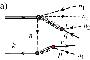
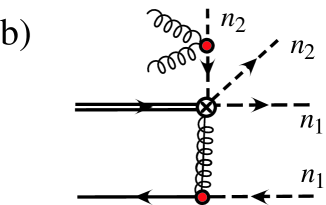
Figure -1137: Graphs which generate a strong phase in lowest order matching of ${\rm SCET}_{\rm I}$ operators onto ${\rm SCET}_{\rm II}$: a) has a $Q^{(1)}$, two ${\cal L}_{\xi_{n_{1}}q}^{(1)}$, and one ${\cal L}_{\xi_{n_{2}}q}^{(1)}$ and contributes to the annihilation amplitude at ${\cal O}(\alpha_{s}^{2}(\mu_{i}))$; and b) has a $Q^{(1)}$, one ${\cal L}_{\xi_{n_{1}}q}^{(1)}$, and one ${\cal L}_{\xi_{n_{2}}\xi_{n_{2}}}^{(2)}$ and contributes to non-annihilation amplitudes at ${\cal O}(\alpha_{s}(\mu_{i}))$. Dashed quark lines are $n_{1}$ or $n_{2}$ collinear, and solid quark lines are soft.

We close this section by giving two examples of time-ordered products generating the nonperturbative strong phases discussed above. We consider a time-ordered product with three ${\cal L}^{(1)}_{\xi q}$ insertions contributing to annihilation. When matching onto ${\rm SCET}_{\rm II}$ we integrate out the hard-collinear modes, leading to an eight-quark operator. Figure -1137a shows the order $\alpha_{s}^{2}(\mu_{i})$ contribution to this matching. The soft quark lines remain open as their contraction leads to an on-shell line which must be treated nonpertrubatively. The resulting ${\rm SCET}_{\rm II}$ operator has the generic form

$$O^{II} =J(n_{2}\cdot p,n_{1}\cdot l,n_{1}\cdot r,n_{2}\cdot q,n_{1}\cdot k)$$ (50)

$$\quad\times(\bar{q}_{s}S_{n_{1}})_{n_{1}\cdot r}\,\Gamma^{(1)}(S_{n_{2}}^{\dagger}q_{s})_{n_{2}\cdot q}\,(\bar{q}_{s}S_{n_{2}})_{n_{1}\cdot k}\,\Gamma^{(2)}(S^{\dagger}_{n_{1}}h_{v})\,(\bar{q}_{n_{1},l}\Gamma^{(3)}q_{n_{1},l^{\prime}})\,(\bar{q}_{n_{2},p^{\prime}}\Gamma^{(4)}q_{n_{2},p})$$

where we use the shorthand subscript notation, $(S_{n_{i}}^{\dagger}q_{s})_{n_{i}\cdot q}\equiv[\delta(n_{i}\!\cdot\!q-n_{i}\!\cdot\!{\cal P})S_{n_{i}}^{\dagger}q_{s}]$. We took the jet directions to be $n_{1}$ and $n_{2}$, rather than $n$ and $\bar{n}$, to emphasize that the soft operator is sensitive to the relative directions of the jets. The functions $S_{i}$ shown in Table 1 are defined by the matrix element of this type of operator

$$S_{i}(n_{1}\!\cdot\!k,n_{1}\!\cdot\!r,n_{2}\!\cdot\!q,)\equiv\langle 0|(\bar{q}_{s}S_{n_{1}})_{n_{1}\cdot r}\,\Gamma_{i}^{(1)}(S_{n_{2}}^{\dagger}q_{s})_{n_{2}\cdot q}\,(\bar{q}_{s}S_{n_{2}})_{n_{1}\cdot k}\,\Gamma_{i}^{(2)}(S^{\dagger}_{n_{1}}h_{v})|B(v)\rangle\,,$$ (51)

where $i$ runs over color, Dirac, and flavor structures. To count the factors of $\pi$ in these amplitudes, note that the hard-collinear contractions give $g^{4}$, and that the matrix element of the resulting four-quark operator, $\langle 0|(\bar{q}\ldots q)(\bar{q}\ldots b_{v})|B\rangle$, is suppressed by $1/(4\pi)^{2}$ relative to $\langle 0|(\bar{q}\ldots b_{v})|B\rangle$. (The four-quark operator has an extra loop with no extra couplings.) This demonstrates that nonperturbative complex contributions first occur at order $[\alpha_{s}(\mu_{i})^{2}/\pi](\Lambda/m_{b})$, i.e., suppressed by $[\alpha_{s}(\mu_{i})/\pi](\Lambda/m_{b})$ compared to the leading amplitudes. The phases arising from the type of matrix element shown in Eq. (51) play a crucial role in explaining the observed strong phases which arise in color suppressed decays Mantry:2003uz . Their resulting operators predict the equality of amplitudes and strong phases between decays involving $D$ and $D^{*}$ mesons and have been confirmed in the data Pirjol:2004yf . This type of diagrams also have long-distance contributions of the same order, which arise from time-ordered products in ${\rm SCET}_{\rm II}$ and can also be complex. To see this note that the hard-collinear quark propagator in Fig. -1137a could also be on-shell (i.e., have ${\cal O}(\Lambda^{2})$ virtuality), in which case it would remain open until the matrix element is taken at the low scale. By opening that line we see that this contribution corresponds to the time-ordered product of a four-quark operator and a six-quark operator, both of which are generated when matching onto ${\rm SCET}_{\rm II}$. A long-distance part is the same order in $\alpha_{s}(\mu_{i})$ and does not change our conclusions about these terms. In Fig. -1137b we show a non-annihilation contribution to $\hat{A}_{rest}^{(1)}$ which is of order $\alpha_{s}(\mu_{i})\Lambda/m_{b}$. This term is generated by the time-ordered product of $Q^{(1)}$, an insertion of the $n_{1}$-collinear ${\cal L}_{\xi q}^{(1)}$, and an operator with $n_{2}$-collinear quarks and usoft gluons,

$${\cal L}_{\xi\xi}^{(2)}=(\bar{\xi}_{n}W)\,Y_{n_{2}}^{\dagger}iD\!\!\!\!/_{us}^{\perp}\,iD\!\!\!\!/_{us}^{\perp}Y_{n_{2}}\,\frac{\not{\bar{n}}}{2\bar{\cal P}}\,(W^{\dagger}\xi_{n})\,.$$ (52)

VI Applications and Conclusion

VI.1 Phenomenological Implications

To understand the implications of the experimental data, it is crucial to know which contributions to the $B\to M_{1}M_{2}$ amplitudes can be complex. The best sensitivity to non-SM physics is via interference phenomena, where new interactions enter linearly (instead of quadratically), such as $CP$-violating observables. The sensitivity to such effects depends on how well we understand the dominant and subdominant SM amplitudes, including their strong phases. The existence of strong phases in $B$ decays is experimentally well established (e.g., the $B\to D\pi$ and $B\to\pi\pi$ rates, the $CP$ asymmetry $A_{K^{+}\pi^{-}}$, the transversity analysis in $B\to J/\psi K^{*}$, etc.).

One example of how strong phase information can be useful is the method for determining $\gamma$ from $B\to\pi\pi$ proposed in Ref. Bauer:2004dg . The method uses isospin, the factorization prediction that ${\rm Im}(C/T)\sim{\cal O}\big{(}\alpha_{s}(m_{b}),{\Lambda}/{m_{b}}\big{)}$, and does not require data on the poorly measured direct $CP$ asymmetry $C_{\pi^{0}\pi^{0}}$. The phases in $A^{(0)}$ at $\alpha_{s}(m_{b})\alpha_{s}(\mu_{i})$ are calculable and partially known BBNS ; Beneke:2005vv . The current $B\to\pi\pi$ data is in mild conflict (at the $\sim 2\sigma$ level) with the SM CKM fit Grossman:2005jb . More precise measurements are needed to understand how well the theoretical expectations are satisfied, and to decipher whether there might be a hint for new physics. Obviously further information about power corrections in ${\rm Im}(C/T)$ could help to clarify the situation.

In all factorization-based approaches to charmless $B$ decays, several parameters are fit from the data or are allowed to vary in certain ranges. The choice and ranges of these parameters should be determined by the power counting. This motivated keeping the charm penguin amplitudes, $A_{c\bar{c}}$ as free parameters in SCET Bauer:2004tj , as was done earlier in Ref. Ciuchini . In the BBNS approach these are argued to be factorizable BBNS . A fit to the data using this parameterization found large power suppressed effects Charles:2004jd including annihilation amplitudes, which might be interpreted as a breakdown of the $\Lambda/m_{b}$ expansion. In QCD sum rules, the annihilation amplitude was found to be of the expected magnitude and to have a sizable strong phase Khodjamirian:2005wn , but a distinction between the terms we identify as real local annihilation and complex time-ordered product annihilation was not made.

Channels like $B\to K\pi$ and $B\to K\bar{K}$ are sensitive to new physics, but by the same token are dominated by penguin amplitudes, which can have charm penguin, annihilation, and other standard model contributions. Since there are possible large nonperturbative $c$-loop contributions in $A_{c\bar{c}}$ that have the same $SU(3)$ flavor transformation properties as annihilation terms, they cannot be easily distinguished by simple fits to the data. However, in a systematic analysis based on SCET these correspond to different operators’ matrix elements, so it is possible to disentangle the various contributions and determine their expected size. The factorization theorems for annihilation amplitudes derived here only involve distributions that already occurred at leading order. This means that we can compare the size of annihilation amplitudes to experimental data without further ambiguities from additional hadronic parameters. We take up this comparison in section VI.2 below.

As an explicit example of how to assemble our results in sections III and IV, we derive the local annihilation amplitude for $\bar{B}^{0}\to K^{-}\pi^{+}$. From Table 2 we can read off the result for this channel, $H(x,y)=-a_{4}^{s}(x,y)-a_{8}^{s}(x,y)$, and from Table 4, $H_{\chi 1}=-a_{1}^{\chi}(x,y)+1/2\,a_{5}^{\chi}(x,y)$ and $H_{\chi 2}=a_{2}^{\chi}(x,y)-1/2\,a_{6}^{\chi}(x,y)$. With the lowest order matching results in Eqs. (III) and (IV) we can set $a_{8}=0$ and $a_{4u}=a_{4c}$, which inserted into Eqs. (23) and (IV) gives

$$A_{Lann}^{(1)}(K^{-}\pi^{+}) =\frac{G_{F}f_{B}f_{\pi}f_{K}}{\sqrt{2}}\,(\lambda_{c}^{(s)}\!+\!\lambda_{u}^{(s)})\int\!\!dx\,dy\,a_{4u}(x,y)\phi^{\pi}(y)\phi^{K}(x)$$ (53)

$$=\frac{G_{F}f_{B}f_{\pi}f_{K}}{\sqrt{2}}\,(\lambda_{c}^{(s)}\!+\!\lambda_{u}^{(s)})\,\beta_{4u}^{\pi K}\,,$$

$$A_{Lann}^{(2)}(K^{-}\pi^{+}) =\frac{G_{F}f_{B}f_{\pi}f_{K}}{6\sqrt{2}}\,(\lambda_{c}^{(s)}\!+\!\lambda_{u}^{(s)})\int\!\!dx\,dy\,\Big{[}\frac{\mu_{\pi}}{m_{b}}\,\Big{\{}a_{1}^{\chi}(x,y)-\frac{1}{2}a_{5}^{\chi}(x,y)\Big{\}}\phi_{pp}^{\pi}(y)\phi^{K}(x)$$

$$\qquad\qquad-\frac{\mu_{K}}{m_{b}}\,\Big{\{}a_{2}^{\chi}(x,y)-\frac{1}{2}a_{6}^{\chi}(x,y)\Big{\}}\phi^{\pi}(y)\phi_{pp}^{K}(x)\Big{]}$$

$$=\frac{G_{F}f_{B}f_{\pi}f_{K}}{\sqrt{2}}\,(\lambda_{c}^{(s)}\!+\!\lambda_{u}^{(s)})\Big{[}\frac{\mu_{\pi}}{m_{b}}\,\Big{\{}\beta_{\chi 1}^{\pi K}-\frac{1}{2}\beta_{\chi 5}^{\pi K}\Big{\}}-\frac{\mu_{K}}{m_{b}}\,\Big{\{}\beta_{\chi 2}^{\pi K}-\frac{1}{2}\beta_{\chi 6}^{\pi K}\Big{\}}\Big{]}\,.$$

Thus, both the leading order annihilation amplitude $A^{(1)}_{Lann}$, and the chirally enhanced annihilation amplitude $A^{(2)}_{Lann}$ are determined by the $\beta$’s defined in Eqs. (III) and (IV). Other $K\pi$ channels have similar expressions with different Clebsch-Gordan coefficients. To the local annihilation contributions we must add the hard-collinear annihilation terms computed in Ref. Arnesen2 , $A_{\rm hard-collin}^{(1ann)}$, since they are the same order in $\alpha_{s}$ and $1/m_{b}$ as the $A_{Lann}^{(1)}$ terms. To see explicitly what the $\beta$’s involve we insert the ${\cal O}(\alpha_{s})$ values of $a_{3u}(x,y)$, $a_{1}^{\chi}(x,y)$, and $a_{2}^{\chi}(x,y)$ to give

$$A_{Lann}(K^{-}\pi^{+})=-\frac{G_{F}f_{B}f_{M_{1}}f_{M_{2}}}{\sqrt{2}}(\lambda_{c}^{(s)}+\lambda_{u}^{(s)})\frac{4\pi\alpha_{s}(\mu_{h})}{9}$$

$$\quad\times\bigg{\{}\Big{(}\frac{C_{9}}{6}-\frac{C_{3}}{3}\Big{)}\Big{[}\big{\langle}\bar{x}^{-2}\big{\rangle}^{K}\big{\langle}y^{-1}\big{\rangle}^{\pi}-\big{\langle}[y(x\bar{y}-1)]^{-1}\big{\rangle}^{\pi K}+d(\mu_{-})\phi_{K}^{\prime}(1)\langle y^{-1}\big{\rangle}^{\pi}\Big{]}$$

$$\qquad-\frac{2\mu_{\pi}}{3m_{b}}\Big{(}{C_{6}}\!-\!\frac{C_{8}}{2}\!+\!\frac{C_{5}}{3}\!-\!\frac{C_{7}}{6}\Big{)}\Big{[}\big{\langle}y^{-2}\bar{y}^{-1}\big{\rangle}_{pp}^{\pi}\big{(}\big{\langle}\bar{x}^{-2}\big{\rangle}^{K}\!+\!\big{\langle}\bar{x}^{-1}\big{\rangle}^{K}\big{)}+d_{1}(\mu_{-})\phi_{K}^{\prime}(1)\big{\langle}y^{-2}\bar{y}^{-1}\big{\rangle}_{pp}^{\pi}$$

$$\qquad\ \ \ -d_{2}(\mu_{+})\phi_{\pi}^{\prime}(0)\big{(}\big{\langle}\bar{x}^{-2}\big{\rangle}^{K}\!+\!\big{\langle}\bar{x}^{-1}\big{\rangle}^{K}\big{)}-d_{3}(\mu_{\pm})\phi_{K}^{\prime}(1)\phi_{\pi}^{\prime}(0)\Big{]}$$

$$\qquad-\frac{2\mu_{\pi}}{3m_{b}}\Big{(}\frac{C_{5}}{3}\!-\!\frac{C_{7}}{6}\Big{)}\big{\langle}[(1-x\bar{y})\bar{x}y^{2}]^{-1}\big{\rangle}^{\pi K}_{pp}+\frac{2\mu_{K}}{3m_{b}}\Big{(}\frac{C_{5}}{3}\!-\!\frac{C_{7}}{6}\Big{)}\big{\langle}[(1-x\bar{y})\bar{x}^{2}y]^{-1}\big{\rangle}_{pp}^{K\pi}$$

$$\qquad-\frac{2\mu_{K}}{3m_{b}}\Big{(}{C_{6}}\!-\!\frac{C_{8}}{2}\!+\!\frac{C_{5}}{3}\!-\!\frac{C_{7}}{6}\Big{)}\Big{[}\big{(}\big{\langle}y^{-2}\big{\rangle}^{\pi}+\big{\langle}y^{-1}\big{\rangle}^{\pi}\big{)}\big{\langle}x^{-1}\bar{x}^{-2}\big{\rangle}^{K}_{pp}-d_{1}(\mu_{+})\phi_{\pi}^{\prime}(0)\big{\langle}\bar{x}^{-2}x^{-1}\big{\rangle}_{pp}^{K}$$

$$\qquad\ \ \ +d_{2}(\mu_{-})\phi_{K}^{\prime}(1)\big{(}\big{\langle}y^{-2}\big{\rangle}^{\pi}\!+\!\big{\langle}y^{-1}\big{\rangle}^{\pi}\big{)}-d_{3}(\mu_{\pm})\phi_{\pi}^{\prime}(0)\phi_{K}^{\prime}(1)\Big{]}\bigg{\}}.$$ (54)

Here results for the convolutions denoted by brackets $\langle\cdots\rangle$ can be found in Eqs. (III), (33), (46), and (IV) in the minimal subtraction scheme. Results for other channels can be assembled in a similar fashion. Corrections to $A_{Lann}+A_{\rm hard-collin}^{(1ann)}$ are suppressed by ${\cal O}[\alpha_{s}^{2}(\mu_{i})/(\pi\alpha_{s}(m_{b}))]$, while we caution that additional $\alpha_{s}(\mu_{h})\Lambda/m_{b}$ terms without a $\mu_{\pi}$ or $\mu_{K}$ will be present in the last two lines of Eq. (VI.1). In the next subsection we derive results for all of these channels using a simple model for the distribution functions, and study numerically the size of the annihilation amplitudes.

Annihilation contributions have been claimed to play important roles in several observables Keum ; Keum:2000wi ; BBNS2 ; BN ; alex , in particular in generating large strong phases in $B\to K\pi$ decays Keum ; Keum:2000wi . The $B\to\pi\pi$ and $K\pi$ data indicate that the latter decays are dominated by penguin amplitudes, and the pattern of rates and $CP$ asymmetries is not in good agreement with some predictions. In particular, it is not easy in the BBNS analysis to accommodate the measured $CP$ asymmetry, $A_{K^{+}\pi^{-}}=-0.108\pm 0.017$ HFAG , except in the S3 and S4 models of Ref. BN . In these models the annihilation contributions are included by using asymptotic distributions, and divergent integrals are parameterized as $\int_{0}^{1}dx/x\to X_{A}$ and $\int_{0}^{1}dx\ln x/x\to-X_{A}^{2}/2$, with $X_{A}=(1+\varrho_{A}e^{i\varphi_{A}})\ln(m_{B}/500\,{\rm MeV})$. Model S3 postulates $\varrho_{A}=1$, $\varphi_{A}=-45^{\circ}$ for all final states, while in the S4 scenario $\varrho_{A}=1$ and $\varphi_{A}=-55^{\circ},\,-20^{\circ},\,-70^{\circ}$ for the $PP,\,PV,\,VP$ channels, respectively. Thus

$$S3:\ X_{A}=4.0-1.7\,i\,,\qquad S4:\ X_{A}=\{3.7-1.9\,i\>,\>4.6-0.8\,i\>,\>3.2-2.2\,i\}\,.$$ (55)

In addition, $\alpha_{s}(\mu)$ and the Wilson coefficients are evaluated at the $\mu_{i}$ intermediate scale BN .

Our result for the factorization of annihilation contributions derived in Sec. III constrains models of annihilation. Equation (23) gives a well defined and real amplitude at leading order, which depends on twist-2 distributions, $\phi_{M}$. It does not involve model parameters $\varrho_{A}$ and $\varphi_{A}$. For $A^{(1)}_{Lann}$ using Eq. (III) and the asymptotic form of the meson distributions, we find a correspondence

$$``X_{A}"=1+\int_{0}^{1}\!dx\,\frac{\phi_{\pi}(x)}{6\,(x^{2})_{\mbox{\o}}}=\ln\Big{(}\frac{m_{b}}{\mu_{+}}\Big{)}\,.$$ (56)

Clearly, $X_{A}$ is real. The asymptotic distributions $\sim 6x(1-x)$ are more accurate for large scales, and at the matching scale where $\mu_{+}\sim m_{b}$, $X_{A}$ is not enhanced by a large logarithm. This matching scale $\mu_{+}$ should not be decreased below $m_{b}$ since $\mu_{+}\sim m_{b}$ is already the correct scale for collinear modes with $p^{+}\sim m_{b}$. We estimate $|X_{A}|\lesssim 1$. Thus, the modeling of annihilation contributions with complex $X_{A}$ in the BBNS approach (including the phenomenologically favored S3 and S4 scenarios) are in conflict with the heavy quark limit, and should be constrained to give smaller real $X_{A}$’s.

In the KLS Keum treatment of annihilation, complex amplitudes are generated from dynamics at the intermediate scale from the $i\epsilon$ in propagators. The MS-factorization used in the derivation of our annihilation amplitudes demonstrates that including the $i\epsilon$ term in collinear factorization would induce a double counting. Thus we expect such contributions to physical strong phases to be realized by operators with soft exchange that occur at higher order in $\Lambda/m_{b}$ and therefore to be small.

Annihilation contributions were also argued to play an important role in explaining the large transverse polarization fraction in $B\to\phi K^{*}$ alex . It was shown that factorization implies $R_{T}={\cal O}(1/m_{b}^{2})$, where $R_{T}$ denotes the transverse polarization fraction alex . Subsequently, it was shown using SCET that $R_{T}$ is power suppressed unless a long-distance charm penguin amplitude $A_{c\bar{c}}$ spoils this result Bauer:2004tj ; Williamson:2006hb . Experimentally, one finds $R_{T}(B\to\phi K^{*})\approx 0.5$ HFAG , while $R_{T}(B\to\rho\rho)$ is at the few percent level. It has been argued that the large $R_{T}(B\to\phi K^{*})$ may provide a hint of new physics in the $b\to s\bar{s}s$ channel. In Ref. alex it was suggested that standard model annihilation contributions may account for the observed large value of $R_{T}(B\to\phi K^{*})$. Our analysis in Sec. IV agrees with alex in that annihilation contributions to the transverse polarization amplitude at first order in $\alpha_{s}$ are suppressed by not one, but two powers of $\Lambda/m_{b}$. However, we do not find a numerical enhancement of these terms (which in alex is partly due to the large sensitivity of the $(2X_{A}-3)(1-X_{A})$ function to $\varrho_{A}$ in the BBNS parameterization). The operators in Eq. (IV) give rise to transverse polarization, but since MS-factorization renders the naively divergent convolutions finite, these power suppressed amplitudes do not receive sizable enhancements. Although we have not derived explicit results for the $B\to\phi K^{*}$ annihilation amplitudes (since $\phi$ is an isosinglet), our results make it unlikely that local annihilation can explain the $R_{T}(B\to\phi K^{*})$ data. We have not explored whether the time-ordered products at ${\cal O}(\alpha_{s}^{2}(\mu_{i})\Lambda/m_{b})$ could give rise to transverse polarization, and it would be interesting to do so.

VI.2 Annihilation amplitudes with simple models for $\phi^{M}(x)$ and $\phi_{pp}^{M}(x)$

In this section we derive numerical results for the local annihilation amplitudes in various channels using a simple model for the distributions. It is convenient to write the $\Delta S=0$ local annihilation amplitude as

$$A_{Lann}(\bar{B}\to M_{1}M_{2}) =-\frac{G_{F}f_{B}f_{M_{1}}f_{M_{2}}}{\sqrt{2}}\>\bigg{\{}\lambda^{(d)}_{u}h_{u}(\bar{B}\to M_{1}M_{2})+\lambda^{(d)}_{c}h_{c}(\bar{B}\to M_{1}M_{2})$$

$$+(\lambda^{(d)}_{u}+\lambda^{(d)}_{c})\Big{[}\frac{\mu_{M_{1}}}{m_{b}}\>h_{\chi 1}(\bar{B}\to M_{1}M_{2})+\>\frac{\mu_{M_{2}}}{m_{b}}\>h_{\chi 2}(\bar{B}\to M_{1}M_{2})\Big{]}\bigg{\}}\,.$$ (57)

For $\Delta S=1$ decays we replace $\lambda^{(d)}_{u,c}\to\lambda^{(s)}_{u,c}$. The coefficients $h_{u}$, $h_{c}$, $h_{\chi 1}$, and $h_{\chi 2}$ are equal to linear combinations of $\beta_{iu}$, $\beta_{ic}$, $\beta_{\chi 1}$, $\beta_{\chi 2}$, $\beta_{\chi 5}$, and $\beta_{\chi 6}$ with Clebsch-Gordan coefficients determined from Tables 2, 3, 4, 5. The combinations are simply determined by the replacements

$$h_{u} =\big{(}H(x,y)\mbox{ with }\tilde{a}_{i}^{d,s}(x,y)\to\beta_{iu}^{M_{1}M_{2}},\ \tilde{a}_{i}^{d,s}(y,x)\to\beta_{iu}^{M_{2}M_{1}}\big{)}\,,$$

$$h_{c} =\big{(}H(x,y)\mbox{ with }\tilde{a}_{i}^{d,s}(x,y)\to\beta_{ic}^{M_{1}M_{2}},\ \tilde{a}_{i}^{d,s}(y,x)\to\beta_{ic}^{M_{2}M_{1}}\big{)}\,,$$

$$h_{\chi 1} =\big{(}H_{\chi 1}(x,y)\mbox{ with }a_{1,5}^{\chi}(x,y)\to\beta_{\chi 1,\chi 5}\big{)}\,,$$

$$h_{\chi 2} =\big{(}H_{\chi 2}(x,y)\mbox{ with }a_{2,6}^{\chi}(x,y)\to\beta_{\chi 2,\chi 6}\big{)}\,.$$ (58)

For the coefficients $a_{3u,3c,4u,4c,7,8}$ and the $a_{i}^{\chi}$’s, the ${\cal O}(\alpha_{s}^{2}C_{1,2})$ matching corrections could be comparable numerically with the ${\cal O}(\alpha_{s}C_{3-10})$ corrections considered here. This should be kept in mind when examining numbers quoted below for the corresponding $\beta$’s.

Results for the coefficients $\beta_{iu}$, $\beta_{ic}$, and $\beta_{\chi i}$, can be found in Eqs. (III) and (IV). To derive numerical results we need to model the meson distribution functions. We take the $C_{i}$ from Eq. (II), use

$$\alpha_{s}(\mu_{h}) =0.22\,, \mu_{\pi}(\mu_{h}) =2.3\,{\rm GeV}\,, \mu_{K}(\mu_{h}) =2.7\,{\rm GeV}\,,$$

$$f_{K} =0.16\,{\rm GeV}, f_{\pi} =0.13\,{\rm GeV}, f_{B} =0.22\,{\rm GeV},$$ (59)

where $\mu_{h}=m_{b}=4.7\,{\rm GeV}$, $f_{B}$ comes from a recent lattice determination Gray:2005ad . For the $\phi$’s we take simple models with parameters $a_{i}^{M}$ and $a_{ipp}^{M}$ which we consider specified at the high scale $\mu_{h}$,

$$\phi^{M}(x) =6x(1-x)\big{[}1+a_{1}^{M}(6x-3)+6a_{2}^{M}(1-5x+5x^{2})\big{]}\,,$$

$$\phi_{pp}^{P}(x) =6x(1-x)\big{[}1+a_{1pp}^{P}(6x-3)+6a_{2pp}^{P}(1-5x+5x^{2})\big{]}\,.$$ (60)

Based on recent lattice data for moments of the $\pi$ and $K$ distributions Braun:2006dg we take $a_{2}^{\pi,K}=0.2\pm 0.2$, where the lattice error was doubled to give some estimate for higher moments. For the $\pi$ we set $a_{1}^{\pi}=a_{1pp}^{\pi}=0$, while for the $K$ we use Braun:2006dg $a_{1}^{K}=0.05\pm 0.02$. We also take $w_{3\pi,K}=-3\pm 1$, $a_{2pp}^{\pi,K}=0\pm 0.4$ and $a_{1pp}^{K}=0.0\pm 0.2$. Note that the range for our parameters is similar to those used in the BBNS models BBNS2 ; BN and light-cone sum rules Ball:2006wn . Since the uncertainties in the model parameters are large and not significantly affected by variation of the $\mu_{\pm}$ scales we keep these fixed at $m_{b}$, where the logs in the $d_{i}(\mu_{\pm})$ terms drop out and the constant under the logs are neglected. A scan over models with parameters in these limits gives predictions for the annihilation coefficients. For the $\bar{B}\to K\pi$ channels we find

$$\beta_{2u}^{\pi K} =1.8\pm 1.2, \beta_{4u}^{\pi K} =\beta_{4c}^{\pi K}=-0.15\pm 0.10, \beta_{2c}^{\pi K} =0.14\pm 0.09\,,$$

$$\beta_{hc1}^{\pi K} =0.09\pm 0.33, \beta_{hc2}^{\pi K} =-0.29\pm 0.09,\ \ \beta_{hc3}^{\pi K}=-0.012\pm 0.002, \beta_{hc4}^{\pi K} =0.002\pm 0.01\,,$$

$$\beta_{\chi 1}^{\pi K} =0.0\pm 6.5, \beta_{\chi 2}^{\pi K} =0.0\pm 5.8,\ \ \beta_{\chi 5}^{\pi K}=0.0\pm 0.094, \beta_{\chi 6}^{\pi K} =0.0\pm 0.11\,.$$ (61)

Using these numbers we can compare the size of the local annihilation amplitudes to the $\bar{B}\to K^{-}\pi^{+}$ data,

$$R_{A}(K^{-}\pi^{+}) =\frac{|A^{(1)}_{Lann}(K^{-}\pi^{+})+A^{(2)}_{Lann}(K^{-}\pi^{+})|}{|A_{Expt.Penguin}(K\pi)|}=0.11\pm 0.09\,,$$

$$R_{A}(\bar{K}^{0}\pi^{-}) =\frac{|A^{(1)}_{Lann}(\bar{K}^{0}\pi^{-})+A^{(2)}_{Lann}(\bar{K}^{0}\pi^{-})|}{|A_{Expt.Penguin}(K\pi)|}=0.12\pm 0.09\,.$$ (62)

For the numerator we did a Gaussian scan using the values from Eq. (VI.2), and determined the error by the standard deviation. For the denominator we used the experimental penguin amplitude determined by a fit to the $B\to K\pi$ data in Ref. Bauer:2005kd . Numerical results for annihilation amplitudes with three-body distribution functions were considered in Ref. Arnesen2 . Although they are similar in size to $A^{(1)}_{Lann}$ they cause only a $\sim 10\%$ change in the value of $R_{A}(K^{-}\pi^{+})$ in Eq. (VI.2). The values of $R_{A}$ indicate that a fairly small portion of the measured penguin amplitude is from annihilation. We do not quote values for the ratio $A_{Lann}^{(2)}/A_{Lann}^{(1)}$, since each of the numerator and denominator can vanish and the parametric uncertainties are very large. For typical values of the parameters in the $K\pi$ channels we find that the $A_{Lann}^{(2)}$ is comparable or even larger than $A_{Lann}^{(1)}$ in agreement with Ref. BBNS2 . The size of the annihilation amplitudes in Eq. (VI.2) are consistent with our expectation for these power corrections. For $B\to\bar{K}K$ we find

$$\beta_{1u}^{\bar{K}K} =-9.6\pm 6.2, \beta_{2u}^{\bar{K}K} =1.7\pm 1.1, \beta_{3u}^{\bar{K}K} =\beta_{3c}^{\bar{K}K}=0.63\pm 0.37,$$

$$\beta_{4u}^{\bar{K}K} =\beta_{4c}^{\bar{K}K}=-0.14\pm 0.09, \beta_{1c}^{\bar{K}K} =-0.03\pm 0.02, \beta_{2c}^{\bar{K}K} =0.13\pm 0.08,$$

$$\beta_{3u}^{K\bar{K}} =\beta_{3c}^{K\bar{K}}=0.63\pm 0.37, \beta_{\chi 1}^{\bar{K}K} =0.0\pm 6.5, \beta_{\chi 2}^{\bar{K}K} =0.0\pm 5.5$$

$$\beta_{\chi 5}^{\bar{K}K} =0.0\pm 0.095, \beta_{\chi 6}^{\bar{K}K} =0.0\pm 0.11\,.$$ (63)

Using these results to determine the $\lambda_{c}^{(d)}$ annihilation contributions to $B\to\bar{K}K$ and comparing this to the experimental penguin amplitude from Ref. Bauer:2005kd gives

$$R_{A}(K^{-}K^{0}) =\frac{|A^{(1)}_{Lann}(K^{-}K^{0})+A^{(2)}_{Lann}(K^{-}K^{0})|}{|A_{Expt.Penguin}(\bar{K}K)|}=0.15\pm 0.11\,.$$ (64)

This is similar in size to the ratios $R_{A}(K^{-}\pi^{+})$, $R_{A}(\bar{K}^{0}\pi^{-})$ and so also consistent with a power correction.

VI.3 Conclusions

In summary, we exhibited how a new factorization in SCET renders the annihilation and “chirally enhanced” annihilation contributions finite in charmless nonleptonic $B\to M_{1}M_{2}$ decays to non-isosinglet mesons. We constructed a complete basis of ${\rm SCET}_{\rm II}$ operators for local annihilation contributions as well as factorization theorems valid to all orders in $\alpha_{s}$. By matching the full QCD diagrams onto ${\rm SCET}_{\rm II}$ operators we showed that their matrix elements are real at leading order in $\Lambda/m_{b}$ and $\alpha_{s}(m_{b})$. The lowest order annihilation contributions depend on $f_{B}$ and a modified type of twist-2 distributions $\phi^{M_{1,2}}$ with dependence on rapidity cutoffs. Chirally enhanced local annihilation contributions depend in addition on modified distributions $\phi^{M_{1,2}}_{pp}$. The annihilation contributions can only have an unsuppressed complex part at ${\cal O}(\Lambda/m_{b})$ if perturbation theory at the intermediate scale, $\sqrt{\Lambda m_{b}}$, breaks down.

In the previous literature models for the power suppressed annihilation corrections were often found to give enhanced contributions with large strong phases, and such assumptions have been important in some fits to the data. Considering all power suppressed amplitudes not involving charm loops, we proved that complex annihilation contributions only occur suppressed by $\alpha_{s}(\sqrt{\Lambda m_{b}})\,\Lambda_{\rm QCD}/m_{b}$ compared to the leading amplitudes. From our factorization theorem we found that annihilation contributes $(11\pm 9)$% of the penguin amplitude in $\bar{B}^{0}\to K^{-}\pi^{+}$, $(12\pm 9)$% in $B^{-}\to\bar{K}^{0}\pi^{-}$, and $(15\pm 11)$% in $B^{-}\to K^{-}K^{0}$. We anticipate that our results will guide future fits to the vast amount of data on charmless $B$ decays, and yield a better understanding of what this data means.

Appendix A Zero-bin subtractions for a two-dimensional distribution

In this appendix we derive a result for the action of the zero-bin subtractions on the integrand obtained from the chirally enhanced annihilation computation, shown in Eq. (IV). Since the result involves a correlation in the $x$ and $y$ integrals it cannot be read off from the results in Ref. Manohar:2006nz . It is convenient to write the momentum fraction factor coming from the offshell $b$-quark propagator as $(1-x\bar{y})=(\bar{x}+y-\bar{x}y)$. Including the rapidity convergence factors Manohar:2006nz , the integral we need is

$$I=\sum_{x\neq 1,\,y\neq 0}\int\!dx_{r}dy_{r}\,\frac{\phi_{pp}^{M_{1}}(y)\phi^{M_{2}}(x)}{(\bar{x}+y-\bar{x}y)\bar{x}y^{2}}\,\Theta_{x}\Theta_{y}\,|x(1-x)|^{\epsilon}\,|y(1-y)|^{\epsilon}\,\Big{(}\frac{\mu_{+}\mu_{-}}{{\bar{n}}\!\cdot\!p_{1}\,n\!\cdot\!p_{2}}\Big{)}^{2\epsilon}\,,$$ (65)

where $\Theta_{x}=\theta(x)\theta(1-x)$. To determine the subtraction terms we must look at the singular behavior as we scale towards the $x=1$ and $y=0$ bins, which we do by taking $\bar{x}\sim\eta$ and $y\sim\eta$. In this limit the gluon and $b$-quark in Fig. -1138 become soft, and this region would be double counted without the zero-bin conditions. First consider the denominator,

$$\frac{1}{\bar{x}+y-\bar{x}y}=\frac{1}{(\bar{x}+y)}+\frac{\bar{x}y}{(\bar{x}+y)^{2}}+\ldots\,.$$ (66)

In the first term the $x$ and $y$ dependence does not decouple, so we must consider them simultaneously. All terms beyond the first one produce finite integrals and are dropped in the minimal subtraction scheme. For the numerator in Eq. (65) we use $\phi_{pp}^{M_{1}}(0)=\phi^{M_{2}}(1)=0$ and expand

$$\phi_{pp}(y)\,\phi(x) =-y\phi_{pp}^{\prime}(0)\,\bar{x}\phi^{\prime}(1)-\frac{y^{2}}{2}\phi_{pp}^{\prime\prime}(0)\,\bar{x}\phi^{\prime}(1)+y\phi_{pp}^{\prime}(0)\,\frac{\bar{x}^{2}}{2}\,\phi^{\prime\prime}(1)+\ldots$$

$$=y\phi_{pp}^{\prime}(0)\sum_{n=1}^{\infty}\frac{(-\bar{x})^{n}}{n!}\,\phi^{(n)}(1)-\frac{y^{2}}{2}\,\phi_{pp}^{\prime\prime}(0)\,\bar{x}\phi^{\prime}(1)+\ldots\,.$$ (67)

In the first term on the last line we have identified all terms which remain singular when multiplied by $1/[\bar{x}y^{2}(\bar{x}\!+\!y)]$. This term is equal to $y\phi_{pp}^{\prime}(0)\phi(x)$. Taken together with the expansion of $\Theta_{x}\Theta_{y}$ we therefore find that the required minimal subtraction is

$$\frac{y\phi_{pp}^{M_{1}\prime}(0)\phi^{M_{2}}(x)}{(\bar{x}+y)\bar{x}y^{2}}\,\Theta_{x}\,\theta(y)\,.$$ (68)

Following Ref. Manohar:2006nz we use this to convert Eq. (65) into an integral that includes the $x=1$ and $y=0$ regions,

$$I =\int_{0}^{1}\!\!dx\int_{0}^{1}\!\!dy\bigg{[}\frac{\phi_{pp}^{M_{1}}(y)\phi^{M_{2}}(x)}{(\bar{x}+y-\bar{x}y)\bar{x}y^{2}}-\frac{y\phi_{pp}^{M_{1}\prime}(0)\phi^{M_{2}}(x)}{(\bar{x}+y)\bar{x}y^{2}}\bigg{]}$$

$$\qquad-\int_{0}^{1}\!\!dx\int_{1}^{\infty}\!\!dy\,\frac{y\phi_{pp}^{M_{1}\prime}(0)\phi^{M_{2}}(x)}{(\bar{x}+y)\bar{x}y^{2}}\,x^{\epsilon}(1-x)^{\epsilon}\,y^{\epsilon}(y-1)^{\epsilon}\,\Big{(}\frac{\mu_{+}\mu_{-}}{{\bar{n}}\!\cdot\!p_{1}\,n\!\cdot\!p_{2}}\Big{)}^{2\epsilon}$$ (69)

$$=\int_{0}^{1}\!\!dx\,\frac{\phi^{M_{2}}(x)}{\bar{x}}\int_{0}^{1}\!\!dy\bigg{[}\frac{\phi_{pp}^{M_{1}}(y)}{(\bar{x}+y-\bar{x}y)y^{2}}-\frac{\phi_{pp}^{M_{1}\prime}(0)}{(\bar{x}+y)y}\bigg{]}-\int_{0}^{1}\!\!dx\!\int_{1}^{\infty}\!\!\!dy\,\frac{\phi_{pp}^{M_{1}\prime}(0)\phi^{M_{2}}(x)}{(\bar{x}+y)\bar{x}y}\,y^{\epsilon}(y-1)^{\epsilon}$$

$$=\int_{0}^{1}\!\!dx\,\frac{\phi^{M_{2}}(x)}{\bar{x}}\int_{0}^{1}\!\!dy\bigg{[}\frac{\phi_{pp}^{M_{1}}(y)}{(\bar{x}+y-\bar{x}y)y^{2}}-\frac{\phi_{pp}^{M_{1}\prime}(0)}{(\bar{x}+y)y}\bigg{]}-\phi_{pp}^{M_{1}\prime}(0)\int_{0}^{1}\!\!dx\,\frac{\phi^{M_{2}}(x)\ln(2-x)}{(1-x)^{2}}\,.$$

Here in simplifying the term carrying the $y\to\infty$ limit, we noted that the integral is finite, and so it does not induce $\mu_{\pm}$ dependence in our subtraction scheme. This result for $I$ was used in Eq. (IV). For the asymptotic pion wave functions, $\phi^{\pi}(x)=6x(1-x)$ and $\phi_{pp}^{\pi}(y)=6y(1-y)$, we obtain $I=36+6\pi^{2}-144\ln 2\,=-4.60$. Note that the steps used here to derive the subtraction also give the correct result for cases where the $x$ and $y$ integrals factorize, such as an integrand $\phi(x)\phi(y)/(x^{2}y^{2})$.

References

• (1) C. W. Bauer, D. Pirjol and I. W. Stewart, Phys. Rev. Lett.  87, 201806 (2001) [hep-ph/0107002].
• (2) M. Beneke, G. Buchalla, M. Neubert and C. T. Sachrajda, Phys. Rev. Lett.  83, 1914 (1999) [hep-ph/9905312]; M. Beneke, G. Buchalla, M. Neubert and C. T. Sachrajda, Nucl. Phys. B 591, 313 (2000) [hep-ph/0006124].
• (3) S. Mantry, D. Pirjol and I. W. Stewart, Phys. Rev. D 68, 114009 (2003) [hep-ph/0306254].
• (4) J. g. Chay and C. Kim, Phys. Rev. D 68, 071502 (2003) [hep-ph/0301055]; Nucl. Phys. B 680, 302 (2004) [hep-ph/0301262].
• (5) C. W. Bauer, D. Pirjol, I. Z. Rothstein and I. W. Stewart, Phys. Rev. D 70, 054015 (2004) [hep-ph/0401188].
• (6) C. W. Bauer, I. Z. Rothstein and I. W. Stewart, hep-ph/0510241.
• (7) Y.Y. Keum, H.n. Li and A.I. Sanda, Phys. Lett. B 504, 6 (2001) [hep-ph/0004004];
• (8) Y. Y. Keum, H. N. Li and A. I. Sanda, Phys. Rev. D 63, 054008 (2001) [hep-ph/0004173].
• (9) C. D. Lu, K. Ukai and M. Z. Yang, Phys. Rev. D 63, 074009 (2001) [hep-ph/0004213].
• (10) M. Beneke, G. Buchalla, M. Neubert and C. T. Sachrajda, Nucl. Phys. B 606, 245 (2001) [hep-ph/0104110].
• (11) M. Beneke and M. Neubert, Nucl. Phys. B 675, 333 (2003) [hep-ph/0308039].
• (12) M. Ciuchini, E. Franco, G. Martinelli and L. Silvestrini, Nucl. Phys. B 501, 271 (1997) [hep-ph/9703353]; M. Ciuchini et al., Phys. Lett. B 515, 33 (2001) [hep-ph/0104126].
• (13) P. Colangelo, G. Nardulli, N. Paver and Riazuddin, Z. Phys. C 45, 575 (1990).
• (14) H. n. Li, hep-ph/0408232.
• (15) T. Feldmann and T. Hurth, JHEP 0411, 037 (2004) [hep-ph/0408188].
• (16) C. W. Bauer, S. Fleming and M. E. Luke, Phys. Rev. D 63, 014006 (2001) [hep-ph/0005275]; C. W. Bauer, S. Fleming, D. Pirjol and I. W. Stewart, Phys. Rev. D 63, 114020 (2001) [hep-ph/0011336]; C. W. Bauer and I. W. Stewart, Phys. Lett. B 516, 134 (2001) [hep-ph/0107001]; C. W. Bauer, D. Pirjol and I. W. Stewart, Phys. Rev. D 65, 054022 (2002) [hep-ph/0109045].
• (17) J. Malcles, hep-ph/0606083; Y. L. Wu and Y. F. Zhou, Phys. Rev. D 72, 034037 (2005) [hep-ph/0503077]; A. J. Buras, R. Fleischer, S. Recksiegel and F. Schwab, Nucl. Phys. B 697, 133 (2004) [hep-ph/0402112]; C. W. Chiang, M. Gronau, J. L. Rosner and D. A. Suprun, Phys. Rev. D 70, 034020 (2004) [hep-ph/0404073].
• (18) A. V. Manohar and I. W. Stewart, hep-ph/0605001.
• (19) C. M. Arnesen, I. Z. Rothstein and I. W. Stewart, Phys. Lett.  B 647, 405 (2007) [arXiv:hep-ph/0611356].
• (20) M. A. Shifman, A. I. Vainshtein and V. I. Zakharov, Nucl. Phys. B 120, 316 (1977).
• (21) G. Buchalla, A. J. Buras and M. E. Lautenbacher, Rev. Mod. Phys.  68, 1125 (1996) [hep-ph/9512380].
• (22) A. J. Buras and L. Silvestrini, Nucl. Phys. B 569, 3 (2000) [hep-ph/9812392].
• (23) A. R. Williamson and J. Zupan, hep-ph/0601214.
• (24) C. W. Bauer, S. Fleming, D. Pirjol, I. Z. Rothstein and I. W. Stewart, Phys. Rev. D 66, 014017 (2002) [hep-ph/0202088].
• (25) C. W. Bauer, D. Pirjol, I. Z. Rothstein and I. W. Stewart, Phys. Rev. D 72, 098502 (2005) [hep-ph/0502094].
• (26) M. Beneke, G. Buchalla, M. Neubert and C. T. Sachrajda, Phys. Rev. D 72, 098501 (2005) [hep-ph/0411171].
• (27) C. W. Bauer, D. Pirjol and I. W. Stewart, Phys. Rev. D 67, 071502 (2003) [hep-ph/0211069].
• (28) B. O. Lange and M. Neubert, Nucl. Phys. B 690, 249 (2004) [Erratum-ibid. B 723, 201 (2005)] [hep-ph/0311345].
• (29) H. n. Li, Czech. J. Phys.  53, 657 (2003) [Prog. Part. Nucl. Phys.  51, 85 (2003)] [hep-ph/0303116].
• (30) C.W. Bauer, D. Pirjol and I.W. Stewart, Phys. Rev. D 68, 034021 (2003) [hep-ph/0303156].
• (31) A. L. Kagan, Phys. Lett. B 601, 151 (2004) [hep-ph/0405134].
• (32) B. O. Lange, A. V. Manohar, I. W. Stewart, in preparation.
• (33) A. Hardmeier, E. Lunghi, D. Pirjol and D. Wyler, Nucl. Phys. B 682, 150 (2004) [hep-ph/0307171].
• (34) V. L. Chernyak and A. R. Zhitnitsky, Phys. Rept.  112, 173 (1984).
• (35) S. Wandzura and F. Wilczek, Phys. Lett. B 72, 195 (1977).
• (36) M. Beneke, A. P. Chapovsky, M. Diehl and T. Feldmann, Nucl. Phys. B 643, 431 (2002) [hep-ph/0206152].
• (37) M. Bander, D. Silverman and A. Soni, Phys. Rev. Lett.  43, 242 (1979).
• (38) T. Becher and R. J. Hill, JHEP 0410, 055 (2004) [hep-ph/0408344].
• (39) S. Mantry, D. Pirjol and I. W. Stewart, AIP Conf. Proc.  722, 141 (2004) [hep-ph/0401058]; D. Pirjol, hep-ph/0411124.
• (40) C. W. Bauer, I. Z. Rothstein and I. W. Stewart, Phys. Rev. Lett.  94, 231802 (2005) [hep-ph/0412120].
• (41) M. Beneke and S. Jager, hep-ph/0512351.
• (42) Y. Grossman, A. Hocker, Z. Ligeti and D. Pirjol, Phys. Rev. D 72, 094033 (2005) [hep-ph/0506228].
• (43) J. Charles et al. [CKMfitter Group], Eur. Phys. J. C 41, 1 (2005) [hep-ph/0406184].
• (44) A. Khodjamirian, T. Mannel, M. Melcher and B. Melic, Phys. Rev. D 72, 094012 (2005) [hep-ph/0509049].
• (45) The Heavy Flavor Averaging Group (HFAG) (E. Barberio et al.), hep-ex/0603003, and updates at http://www.slac.stanford.edu/xorg/hfag/.
• (46) A. Gray et al. [HPQCD Collaboration], Phys. Rev. Lett.  95, 212001 (2005) [hep-lat/0507015].
• (47) V. M. Braun et al., hep-lat/0606012.
• (48) P. Ball, V. M. Braun and A. Lenz, JHEP 0605, 004 (2006) [hep-ph/0603063].