The Rényi entropy $H_{2}$ as a rigorous, measurable lower bound for the entropy of the interaction region in multiparticle production processes

Abstract

A model-independent lower bound on the entropy $S$ of the multi-particle system produced in high energy collisions, provided by the measurable Rényi entropy $H_{2}$, is shown to be very effective. Estimates show that the ratio $H_{2}/S$ remains close to one half for all realistic values of the parameters.

1 Introduction

The evaluation of the entropy of the stuff in the interaction regions of high energy multiparticle production processes is an important problem (cf. e.g. [1],[2] and references given there). Within models, it is possible to estimate this entropy with an uncertainty of about 10% (cf. e.g. [1]). The problem we are addressing in the present paper is, how useful is the model independent lower bound, which can be obtained from experiment using the Rényi entropies.

Even in classical physics it is not easy to measure entropy. While there are simple gadgets to measure temperature, pressure and volume, there is no entropy-meter. The best one can do is to measure changes of entropy. This is reasonably simple for reversible processes in closed systems, when the changes of entropy in a volume are entirely due to the flows of heat across the boundary. In general, however, there are sources of entropy within the volume and these are more difficult to monitor. Moreover, in thermodynamics entropy is primarily defined for equilibrium states. One extends the definition to so-called incomplete equilibria where the system is thought of as consisting of subsystems, each approximately in equilibrium and interacting weakly with each other. Then the total entropy is calculated as the sum of entropies of these subsystems interpreted as systems in equilibrium. It is not quite clear, however, how far from equilibrium one can go without loosing the physical sense of entropy.

Boltzmann proposed the definition of entropy

$$S=-\sum_{i}p_{i}\log p_{i},$$ (1)

where the sum is over all the states of the system, or in more rigorous texts over all the states with non-zero probabilities, and $p_{i}$ is the probability of state $i$. The scale of temperature is chosen here so that the Boltzmann constant equals one. Thus entropy is dimensionless. When the probabilities are given by the canonical ensembles this formula yields the results known from standard thermodynamics; including the third principle of thermodynamics, which states that under some conditions $\lim_{T\rightarrow 0}S(T,\ldots)=0$.

A reinterpretation of formula (1) in terms of information theory was given by Shannon. The result is that the formula can be applied to any probability distribution. In the present paper we deal with the particles produced in high energy collisions of heavy ions. It is not clear how far from equilibrium their distribution is. The possible final states, however, certainly have a probability distribution. Therefore, to be on the safe side, we will refer to Shannon’s entropy, keeping in mind, however, that if the final state is described by the (grand)canonical distribution, this is just Boltzmann’s entropy, or equivalently the entropy known from standard thermodynamics.

2 Estimate of entropy in the interaction region

In order to get a rough estimate of the entropy in the interaction region let us use the following simple model: a perfect gas of identical particles, with mass $m$ each, contained in volume $V$. The temperature $T$ and the chemical potential $\mu$ are given. Thus, neither the energy nor the number of particles is fixed. Maxwell-Boltzmann statistics is used with a factor $\frac{1}{n!}$ in the contribution of each $n$-particle state to the grand partition function. This is sometimes called the quasi-classical approximation. A standard calculation yields formula (22) for the entropy $S(m,V,T,\mu)$. In order to get a number, however, it is necessary to know the values of the four arguments. For the mass of the particle we will take the pion mass. According to an estimate of Pal and Pratt [1], about half the entropy of the system is carried by pions. Here we consider only one kind of pions, thus we estimate about one sixth of the total entropy in the interaction region. The chemical potential is usually put equal zero. For $\mu\rightarrow m$ from below, Einstein’s condensation of the gas takes place and the quasi-classical approximation breaks down. Quantitative estimates of the chemical potential, cf. e.g. [2], [3], [4], give positive values, but sufficiently far from $m$ to make the quasi-classical approximation good within a few per cent. Temperatures are strongly model-dependent. In models where all the transverse momenta are due to thermal motion, they can exceed $200$MeV. In models, where much of the transverse momentum is due to collective motion they can drop to about $100$MeV. For a recent discussion of the temperatures in RHIC experiments see [5]. In the following sections we will consider the region

$$\frac{m}{2}<T<\infty;\qquad-T<\mu<T;\qquad\mu<m.$$ (2)

Here, for comparison with [1], we will use $T=125MeV$ and $\mu=60$MeV, which corresponds to $\frac{\mu}{T}=0.48$.

The estimate of the interaction volume is by far the most difficult part of the problem. The transverse dimensions are usually estimated from the data on Bose-Einstein correlations. There are reasons, however, why these estimates are rather uncertain. Let us mention just two. The phases of the elements of the single-particle density matrix in the momentum representation cannot be determined from momentum measurements. Neglecting these phases one can underestimate the transverse size by a large factor [6]. Guessing them one can err in either direction. Another reason is that according to the standard formula for the diagonal elements of the density matrix in the coordinate representation:

$$\tilde{\rho}(\textbf{x},\textbf{x})=\int\!\!\frac{d^{3}qd^{3}K}{(2\pi)^{3}}\rho(\textbf{K},\textbf{q})e^{i\textbf{qx}},$$ (3)

where $\textbf{q}=\textbf{p - p}^{\prime}$ and $\textbf{K}=\frac{1}{2}(\textbf{p + p}^{\prime})$, the mean squares of the components of x, which characterize the size of the interaction region, are

$$\langle x_{i}^{2}\rangle=-\int\!\!d^{3}K\;\left(\frac{\partial^{2}}{\partial q_{i}^{2}}\rho(\textbf{K},\textbf{q})\right)_{\textbf{q}=0}.$$ (4)

The small q region, however, is experimentally inaccessible. The data have to be extrapolated from larger q regions. It is known that Gaussian extrapolations yield underestimates, but steeper extrapolations can give anything, infinity included. Other measures of the size in ordinary space, e.g. from the half-width of the small $q^{2}$ peak in momentum space, are difficult to interpret. Actually, even if the region $q\approx 0$ were know there would be problems of interpretation. What happens there is strongly affected by the halo of pions produced far away from the decays of long-lived resonances. This would have to be somehow corrected.

The situation for the longitudinal dimension deserves an additional comment. At high energies the total longitudinal size of the interaction region is much larger than the transverse size. In fact, it is believed to increase linearly with $\sqrt{s}$. The volume relevant for the calculation of entropy, however, is the volume at given momentum. In the longitudinal direction this should roughly correspond to the longitudinal size of the homogeneity region, which is obtained from the study of the Bose-Einstein correlations with reservations as for the transverse dimensions. The usual strategy is to calculate entropy densities, or other ratios where the volume cancels. For instance, using formula (22) and the corresponding formula for the particle multiplicity we get

$$\frac{S}{N}=4-\frac{\mu}{T}+\frac{m}{T}\frac{K_{1}\left(\frac{m}{T}\right)}{K_{2}\left(\frac{m}{T}\right)}.$$ (5)

The number four on the right-hand side dominates. Each of the other two is of the order of $0.4$ and, moreover, they tend to cancel. In particular, for $\mu=60$MeV the cancellation is almost exact and

$$\frac{dS}{dy}\approx 4\frac{dN}{dy}.$$ (6)

One could argue that in order to get results at fixed $y$ one should use a two-dimensional momentum distribution. We checked that putting $p_{L}\equiv 0$ one has to replace the coefficient $4$ in this formula by $3.11$. Since, however, for the experimental determination of $dN/dy$ one uses particles from a rather large range of $p_{L}$, we consider the formula in the text more realistic. For the $5$% most central $Au-Au$ collisions at $\sqrt{s}=130$GeV, for the $\pi^{-}$ mesons at midrapidity, the PHENIX collaboration finds $\left(\frac{dN}{dy}\right)_{y=0}=270\pm 3$ [7]. According to [1] this number should be reduced by 12% in order to eliminate the pions from decays of long living resonances. Thus we find

$$\left(\frac{dS}{dy}\right)_{y=0}=961.$$ (7)

Pal and Pratt [1], from a more sophisticated, but closely related, argument find for a sample of less central collisions (centrality $11$%) $\left(\frac{dS}{dy}\right)_{y=0}=680$. For the corresponding sample (centralities from 5% to 15 %) the PHENIX collaboration gives $\frac{dN}{dy}=200\pm 2$, which introduced into (6) yields $\left(\frac{dS}{dy}\right)_{y=0}=704$ in reasonable agreement with the number from [1]. Similarly, using as the density of thermal $\pi^{-}$ mesons one half of the overall $\pi^{-}$ density, as recommended by Akkelin and Sinyukov [2], one obtains from (6), at $\sqrt{s}=130$GeV and $\sqrt{s}=200$GeV respectively, $\frac{dS}{dy}=520$ and $\frac{dS}{dy}=610$ to be compared with 470 and 570 obtained in [2]. The particle densities have been taken from the figures in ref. [2] and averaged over the PHENIX and STAR results.

Let us discuss now the uncertainties of these numbers. The errors quoted here from [7] are statistical. Moreover, there is a systematic error estimated as 13% [7]. In [1] the error is estimated to be about 10%. This error would be quite acceptable, it is model dependent, however . For instance, most crystals at low temperatures have very low entropies (third principle of thermodynamics) and estimating their entropies from a perfect gas model would give results wrong by orders of magnitude. Admittedly, the stuff in the interaction region is not as regular as a crystal at low temperatures, but it is not a perfect gas either. Few would doubt that the perfect gas approximation is better than the low temperature crystal approximation, but how good it actually is, is an open problem. In order to shed some light on this problem it has been proposed by two of us [8] to study the Rényi entropies, which are both measurable and related to Shannon’s entropy. For some more work in this direction see [9], [10] and for a recent review see [11]. Let us now recall some properties of Rényi entropies.

3 Rényi entropies

Let us consider an arbitrary system with states labelled by index $i$. We will explicitly write down formulae for the case when $i$ is discrete, but the generalization to the case when the spectrum of $i$ is continuous, or partly continuous, can be done in the standard way. The Rényi entropy of order $l$ is defined by the formulae

$$H_{l}=\frac{\log C(l)}{1-l};\qquad C(l)=Tr\rho^{l}=\sum_{i}p_{i}^{l},$$ (8)

where $p_{i}$ is the probability of state $i$.

The Rényi entropies have a number of nice features (see e.g. [12]). They are generalizations of Shannon’s entropy, because $H_{1}=S$. They satisfy three out of the four axioms used by Khinchin to derive the formula for Shannon’s entropy, viz. they are functions of the probabilities $p_{i}$, they do not change when a state with zero probability is added and they reach their maximal values when all the probabilities $p_{i}$ are equal (micro-canonical ensemble). It follows from (8) that for the micro-canonical ensemble they coincide with Shannon’s entropy, thus in a way they measure the nonuniformity of the system. Instead of Khinchin’s fourth axiom, which refers to the entropy of a system consisting of subsystems, they all satisfy the weaker condition that when a system consists of independent subsystems the total entropy is the sum of the entropies of the subsystems.

A useful feature of Boltzmann’s entropy, as studied in heavy ion collisons, is that it changes neither during the free streaming of the particles after freeze-out nor during the hydrodynamic expansion, provided this expansion is non dissipative. Rényi entropies do not change in the free streaming process, because they are invariant under the transformation corresponding to the unitary time evolution of the system

\psfrag{aaa}{\Large$\frac{m}{T}$}\psfrag{bbb}{\Large$\frac{1}{N}(H_{2}-S)$}\includegraphics[totalheight=289.07999pt]{how00.eps}

Figure 1: Temperature dependence of the Rényi entropy $H_{2}$ along the reversible adiabate, $S$ = Const, of a perfect gas. The number of particles $N$ is kept constant. The volume cancels.

$$\rho(p,p^{\prime})\rightarrow e^{-iHt}\rho(p,p^{\prime})e^{iHt}.$$ (9)

In fact, as seen from this argument, they are invariant even if the final state interactions are included, provided these interactions can be described e.g. by the Schrödinger equation. They do change, however, when the volume of the system is changed adiabatically and reversibly i.e. in particular in non-dissipative flows. In order to illustrate this point we have calculated the Rényi entropy $H_{2}$ for a perfect gas expanding adiabatically and reversibly, i.e. at constant Shannon entropy. The result is shown in Fig. 1. Since Shannon’s entropy remains constant, the temperature dependence plotted reflects the change of the Rényi entropy $H_{2}$ as a function of temperature. This dependence is not very strong, however. For temperatures changing from very high to $70$MeV the change is by about $0.2$ unit per particle, to be compared with the total entropy of about four units per particle.

There are attempts to build a thermodynamics where the Rényi entropies play the role of Boltzmann’s entropy in standard thermodynamics (cf. e.g. [13]). The motivation is to describe distributions with ”thick tails” which occur often in experiment. Here we will not discuss these possibilities, but use the Rényi entropies as a source of information about Shannon’s entropy. There is a theorem, cf. e.g. [12], that the Rényi entropy $H_{l}$ of a system is a decreasing function of its index $l$. A proof is given in the Appendix. Therefore,

$$S(m,V,T,\mu)>H_{2}(m,V,T,\mu).$$ (10)

Similar inequalities hold also for the Rényi entropies of higher orders, but the corresponding bounds are weaker and, therefore, less useful.

4 Rényi entropies and standard thermodynamics

Let us consider an open, one component system of particles in equilibrium, at temperature $T$ and chemical potential $\mu$. The corresponding grand-canonical probability distribution is

$$p_{i}=\frac{1}{\cal Z}e^{\frac{E_{i}-\mu n_{i}}{T}},$$ (11)

where from the normalization of the probability distribution, the grand partition function

$${\cal Z}=\sum_{i}e^{\frac{E_{i}-\mu n_{i}}{T}}.$$ (12)

The grand partition function is related to the thermodynamic potential $\Omega$ by the formula

$$\Omega(T,V,\mu)=-T\log{\cal Z}.$$ (13)

Potential $\Omega$ is well known in statistical physics. Its relations to other thermodynamical parameters follow from the identity

$$d\Omega=-SdT-pdV-\sum_{\alpha}N_{\alpha}d\mu_{\alpha},$$ (14)

where $\alpha$ labels the kinds of particles in the system. In the following we discuss one component systems, so that the index $\alpha$ is not necessary and we normalize the chemical potential $\mu$ so that $N$ denotes the number of particles in the system. If for arbitrary real, positive $\lambda$

$$\Omega(T,\lambda V,\mu)=\lambda\Omega(T,V,\mu),$$ (15)

as is usually the case when there are no long range interactions, then differentiating both sides of this equation with respect to $\lambda$, putting $\lambda=1$ and using (14) one finds

$$\Omega(T,V,\mu)=-pV.$$ (16)

The probability distribution (11) is a standard concept in the statistical physics of equilibrium states, but also for non-equilibrium states it is considered a reasonable first guess, because it corresponds to no information about the system except for the kind and average number of particles, their average energy and the (fixed) volume [12].

Substituting formula (11) into (8) and using the definition of the potential $\Omega$ one finds

$$H_{l}(T,V,\mu)=\frac{l}{l-1}\frac{1}{T}\left(\Omega(\frac{T}{l},V,\mu)-\Omega(T,V,\mu)\right).$$ (17)

An equivalent formula has been given in [9]. Thus, in general, the Rényi entropy $H_{l}$ is expressed by the thermodynamic functions at two different temperatures $T$ and $T/l$. The only exception is at $l=1$, when the definition of $H_{l}$ yields an indefinite expression of the type $0/0$. For $l\rightarrow 1$, however, one finds the well-known result

$$\lim_{l\rightarrow 1}H_{l}(T,V,\mu)=-\frac{\partial\Omega(T,V,\mu)}{\partial T}=S(T,V,\mu).$$ (18)

5 Gas of non-interacting free particles

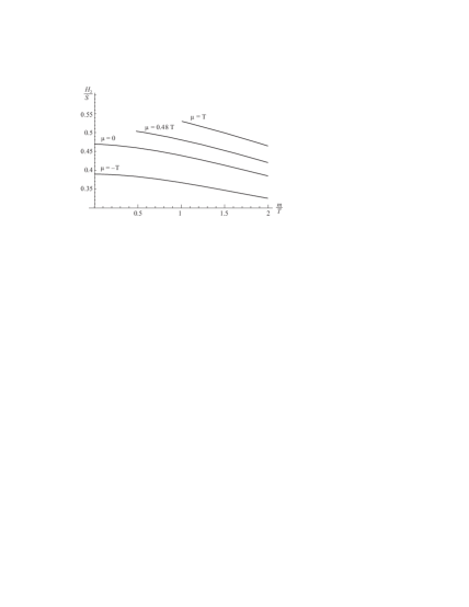
Figure 2: Ratio of the Rényi entropy $H_{2}$ to Shannon’s entropy $S$; Maxwell-Boltzmann statistics. The unphysical results for $\mu>m$ are not included

Let us consider a one component system of free spin zero particles, contained in a fixed volume $V$ and with the Hamiltonian

$$H=\sum_{i=1}^{N}\sqrt{p_{i}^{2}+m^{2}}.$$ (19)

The system is open so that the chemical potential $\mu$ and not the number of particles $N$ is fixed. The state of the system $i$ is specified by giving the number of particles $n_{i}$ in this state and all their momenta. Thus, in the quasi-classical approximation, the grand partition function is

$${\cal Z}(T,V,\mu)=\sum_{n=0}^{\infty}\frac{1}{n!}\left(\frac{Ve^{\frac{\mu}{T}}}{(2\pi\hbar)^{3}}\int\!\!d^{3}p\;e^{-\frac{\sqrt{p^{2}+m^{2}}}{T}}\right)^{n}$$ (20)

Note that the indistinguishability of particles has been taken into account only approximately, by dividing each $n$-particle contribution by $n!$. This is the Maxwell-Boltzmann statistics. As is well known, it is a good approximation when the chemical potential is much smaller than the particle mass. A more general formula based on the Bose-Einstein statistics will be derived latter.

The integral over momenta can be evaluated in spherical coordinates, using the Bessel functions of imaginary argument $K_{\nu}(z)$ (cf. e.g. [14]). The resulting potential $\Omega(T,V,\mu)$ is

$$\Omega(T,V,\mu)=-\frac{m^{2}VT^{2}}{2\pi^{2}\hbar^{3}}e^{\frac{\mu}{T}}K_{2}\left(\frac{m}{T}\right).$$ (21)

The corresponding (Shannon) entropy is

$$S=-\frac{\partial\Omega}{\partial T}=\frac{m^{2}VT}{2\pi^{2}\hbar^{3}}e^{\frac{\mu}{T}}\left[\left(4-\frac{\mu}{T}\right)K_{2}\left(\frac{m}{T}\right)+\frac{m}{T}K_{1}\left(\frac{m}{T}\right)\right].$$ (22)

Substituting the expression for $\Omega(T,V,\mu)$ into formula (17) one finds the Rényi entropies

$$H_{l}(T,V,\mu)=\frac{l}{l-1}\frac{K_{2}\left(\frac{m}{T}\right)-l^{-2}e^{\frac{(l-1)\mu}{T}}K_{2}\left(\frac{lm}{T}\right)}{\left(4-\frac{\mu}{T}\right)K_{2}\left(\frac{m}{T}\right)+\frac{m}{T}K_{1}\left(\frac{m}{T}\right)}S(T,V,\mu).$$ (23)

Let us consider some limiting cases. Using the formula [14] valid for $z\rightarrow 0$ and $\nu>0$

$$K_{\nu}(z)\approx\frac{1}{2}\Gamma(\nu)\left(\frac{2}{z}\right)^{\nu},$$ (24)

one finds that for $m\ll T$ and $km\ll T$

$$H_{l}(T,V,\mu)\approx\frac{l}{l-1}\left(1-l^{-4}e^{(l-1)\frac{\mu}{T}}\right)\frac{1}{4-\frac{\mu}{T}}S(T,V,\mu).$$ (25)

This formula is useful for numerical estimates, because in the limit $m\rightarrow 0$ formula (23) becomes an $\frac{\infty}{\infty}$ expression.

Making the further assumption $\mu\rightarrow 0$ one finds the formula given in [8]

$$H_{l}(T,V,\mu)\approx\frac{1+l^{-1}+l^{-2}+l^{-3}}{4}S(T,V,\mu).$$ (26)

The ratio $\frac{H_{2}(T,V,\mu)}{S(T,V,\mu)}$, calculated numerically from formula (23), is shown in Fig. 2. The values for $\mu>m$ are not shown, because they are unphysical. One should keep in mind, however, that also for $\mu<m$ our method of handling the indistinguishability of massive particles is quantitatively reliable only for $\frac{m-\mu}{T}$ sufficiently large.

The results are rather encouraging. The ratio decreases with increasing $\frac{m}{T}$ and with decreasing $\frac{\mu}{T}$, but even for $\mu=-T$ and $m=2T$ it is still about $0.33$ so that the lower bound underestimates the exact value by a factor of three. At $m=\mu=T$ the ratio reaches its maximum of about $0.53$. This last result, however, should be verfied, because the arguments are beyond the reach of applicability of the Maxwell-Boltzmann statistics. Putting $p_{L}\equiv 0$ one finds qualitatively similar results with the ratio $H_{2}/S$ ranging, in the $\{T,\mu\}$ region considered, from $0.35$ to $0.875$.

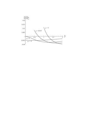
Figure 3: Double ratio $\frac{(H_{2}/S)_{BE}}{(H_{2}/S)_{MB}}$ . The unphysical results for $\mu>m$ are not included.

Let us reconsider now the gas of non-interacting free particles with the Hamiltonian (19), but handling correctly the statistics. The standard method is to use, instead of the states characterized by the number of particles $n_{i}$ and momenta of the $n_{i}$ particles, the occupation numbers $n_{\textbf{p}}$ of all the single particle states. Then

$${\cal Z}(T,V,\mu)=\prod_{\textbf{p}}\left(\sum_{n(\textbf{p})=0}^{\infty}e^{-n(\textbf{p})\frac{E(p)-\mu}{T}}\right)$$ (27)

Summing the geometrical progressions and using the quasi-classical approximation to convert in $\log{\cal Z}$ the summation over momenta into an integration one finds

$$\Omega(T,V,\mu)=\frac{VT}{(2\pi)^{3}}\int\!\!d^{3}p\;\log\left(1-e^{-\frac{E(p)-\mu}{T}}\right).$$ (28)

Expanding the logarithm in powers of the exponential and integrating term by term like in the Maxwell-Boltzmann case one finds

$$\Omega(T,V,\mu)=-\frac{m^{2}VT^{2}}{2\pi^{2}}\sum_{n=1}^{\infty}n^{-2}e^{\frac{n\mu}{T}}K_{2}\left(\frac{nm}{T}\right).$$ (29)

Note that keeping the $n=1$ term only, one reproduces the Maxwell-Boltzmann case. The corresponding Shannon entropy is

$$S(T,V,\mu)=\frac{m^{2}VT}{2\pi^{2}}\sum_{n=1}^{\infty}n^{-2}e^{\frac{n\mu}{T}}\left[\left(4-\frac{n\mu}{T}\right)K_{2}\left(\frac{nm}{T}\right)+\frac{nm}{T}K_{1}\left(\frac{nm}{T}\right)\right].$$ (30)

Let us note the identities

$$\Omega(T,V,\mu)=\sum_{n=1}^{\infty}\Omega_{MB}(\frac{T}{n},V,\mu);\qquad S(T,V,\mu)=\sum_{n=1}^{\infty}n^{-1}S_{MB}(\frac{T}{n},V,\mu),$$ (31)

where the subscript $MB$ denotes the quantities calculated in the Maxwell-Boltzmann approximation. The Rényi entropies are

$$H_{l}(T,V,\mu)=\frac{l}{l-1}\frac{\sum_{n=1}^{\infty}(n)^{-2}e^{\frac{nm}{T}}K_{2}\left(\frac{nm}{T}\right)-\sum_{n=1}^{\infty}(ln)^{-2}e^{\frac{lnm}{T}}K_{2}\left(\frac{lnm}{T}\right)}{\sum_{n=1}^{\infty}n^{-2}e^{\frac{n\mu}{T}}\left[\left(4-\frac{n\mu}{T}\right)K_{2}\left(\frac{nm}{T}\right)+\frac{nm}{T}K_{1}\left(\frac{nm}{T}\right)\right]}S(T,V,\mu).$$ (32)

In Fig. 3 the double ratio $\frac{(H_{2}/S)_{BE}}{(H_{2}/S)_{MB}}$ is shown. It is seen that the ratio of the second Rényi entropy to Shannon’s entropy changes by less than about one per cent when statistics is changed from Maxwell-Boltzmann to Bose-Einstein. On the other hand, as seen from Fig. 4, the entropy itself changes by up to 16%.

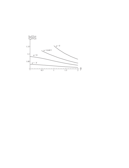
Figure 4: Ratio of Shannon entropies: $\frac{S_{BE}(T,V,\mu)}{S_{MB}(T,V,\mu)}$ The unphysical results for $\mu>m$ are not included.

6 Gas of noninteracting particles in an external potential

The gas studied in the preceding section was confined in a constant volume. It may be more realistic to assume that the volume increases with increasing energy per particle, i.e. with increasing temperature. A model of this type can be obtained by replacing the free particle Hamiltonian (19) by a Hamiltonian including an external potential. We will discuss the simple case of the harmonic oscillator potential:

$$H=\sum_{i=1}^{N}\left(\sqrt{p_{i}^{2}+m^{2}}+\frac{1}{2}K\textbf{x}_{i}^{2}\right),$$ (33)

where $K$ is a constant. Repeating the analysis from the preceding section one finds that in the calculation of $\log{\cal Z}$ the only difference is that the volume $V$ is replaced by

$$V_{eff}(T)=\int\!\!d^{3}x\;e^{-\frac{K\textbf{x}^{2}}{2T}}=V_{0}T^{\frac{3}{2}};\qquad V_{0}=(\frac{2\pi}{K})^{\frac{3}{2}}.$$ (34)

Thus

$$\Omega(T,\mu) = -\frac{m^{2}V_{0}}{2\pi^{2}\hbar^{3}}T^{\frac{7}{2}}K_{2}\left(\frac{m}{T}\right)e^{\frac{\mu}{T}},$$ (35)

$$S(T,\mu) = \frac{m^{2}V_{0}}{2\pi^{2}\hbar^{3}}T^{\frac{5}{2}}\left[K_{2}\left(\frac{m}{T}\right)\left(\frac{11}{2}-\frac{\mu}{T}\right)+\frac{m}{T}K_{1}\left(\frac{m}{T}\right)\right]e^{\frac{\mu}{T}}$$ (36)

and the Rényi entropies are

$$H_{l}(T,\mu)=\frac{l}{l-1}\frac{K_{2}\left(\frac{m}{T}\right)-l^{-\frac{7}{2}}K_{2}\left(\frac{lm}{T}\right)e^{(l-1)\frac{\mu}{T}}}{K_{2}\left(\frac{m}{T}\right)\left(\frac{11}{2}-\frac{\mu}{T}\right)+\frac{m}{T}K_{1}\left(\frac{m}{T}\right)}S(T,\mu).$$ (37)

The ratio $\frac{H_{2}(T,\mu)}{S(T,\mu)}$ is plotted in Fig. 5. It is seen that the presence of the potential reduces the ratio $\frac{H_{2}(T,\mu)}{S(T,\mu)}$. In the region shown in the graph the ratio is between $0.26$ and $0.40$. Qualitatively, the dependence on the parameters is as before.

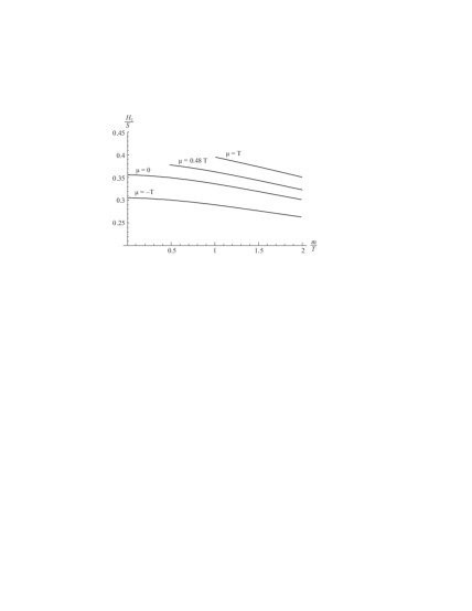
Figure 5: Ratio $H_{2}/S$ for non-interacting particles in the harmonic oscillator potential; quasi-classical approximation. The unphysical results for $\mu>m$ are not included

7 Conclusions

The entropy $S$ is rather difficult to estimate directly from the data. Recently [6], we have proposed a method to measure the Rényi entropy $H_{2}$, which provides a rigorous lower bound for $S$. In the present paper we investigate the relation between $H_{2}$ and $S$ in order to determine how close to the actual value of $S$ this bound is. Using the ideal gas model we find that, for the relevant (rather wide) range of parameters, $H_{2}$ is not far from $\frac{1}{2}S$. The detailed results are presented and discussed in the text. It is found that the ideal gas model reproduces within $10$% the entropy densities obtained by other authors using more sophisticated methods [1], [2]. This suggests that also our estimate of the ratio $H_{2}/S$ should hold in more realistic models. We, therefore, conclude that if the measured Rényi entropy $H_{2}$ turns out to be much smaller than half the entropy $S$ estimated from a model, the model is unlikely to be realistic.

The authors thank Ewa Gudowska-Nowak, Mariusz Sadzikowski and Karol Życzkowski for discussions and Yuri Sinyukov for calling their attention to ref. [2].

8 Appendix

The Rényi entropy $H_{l}$ is a decreasing function of the index $l$. This can be seen as follows (cf. [12]). Differentiating both sides of the definition (8) with respect to $l$ we get

$$\frac{dH_{l}}{dl}=-(1-l)^{2}\sum_{i}P_{i}\log\frac{P_{i}}{p_{i}},$$ (38)

where the notation

$$P_{i}=\frac{p_{i}^{l}}{\sum_{i}p_{i}^{l}}$$ (39)

has been introduced. Using the identity

$$\log x\geq 1-\frac{1}{x},$$ (40)

where equality holds only when $x=1$, one easily checks that for all $l\neq 1$ the right-hand side is non-positive. Actually, it is negative unless all the probabilities $p_{i}$ are equal, which is not the case for multiple particle production processes.

References

- [1] S. Pal and S. Pratt, Phys. Lett. B578(2004)310.
- [2] S.V. Akkelin and Yu. M. Sinyukov, nucl-th/0505045v4(2006).
- [3] B. Tomasik and U.A. Wiedemann, Phys.Rev. C68(2003)034905.
- [4] S.V. Akkelin and Yu.M. Sinyukov, Phys. Rev. C70(2004)064901.
- [5] M. Biyajima et al., hep-ph/0602120.
- [6] A. Bialas and K.Zalewski, Phys. Rev. D72(2005)0306009.
- [7] K. Adcox et al., Phys. Rev. Lett. 88(2002)242301.
- [8] A. Bialas and W. Czyz, Phys. Rev. D61(2000)074021.
- [9] A. Bialas and W. Czyz, Acta Phys. Pol. B31(2000)2803.
- [10] A. Bialas and W. Czyz, Acta Phys. Pol. B31(2000)687, Acta Phys. Pol. B34(2003)3363, A. Bialas, W.Czyz and K. Zalewski, Acta Phys. Pol. B36(2005)3109, Phys. Lett. B633(2006)479, A. Bialas and K. Zalewski, Phys. Rev. C73(2006)034912, Acta Phys. Pol. B37(2006)495.
- [11] A. Bialas and K.Zalewski, hep-ph/0602059.
- [12] C. Beck and F. Schlögl, Thermodynamics of chaotic systems, an introduction, Cambridge University Press (1993).
- [13] A.S. Parvan and T.S. Biro, Phys. Lett. A340(2005)375.
- [14] M. Abramowitz and I.A. Stegun, (eds), Handbook of mathematical functions, Dover Publications, New York (1968),