Ultra high energy neutrino-nucleon cross section from
cosmic ray experiments and neutrino telescopes

Abstract

We deduce the cosmogenic neutrino flux by jointly analysing ultra high energy cosmic ray data from HiRes-I and II, AGASA and the Pierre Auger Observatory. We make two determinations of the neutrino flux by using a model-dependent method and a model-independent method. The former is well-known, and involves the use of a power-law injection spectrum. The latter is a regularized unfolding procedure. We then use neutrino flux bounds obtained by the RICE experiment to constrain the neutrino-nucleon inelastic cross section at energies inaccessible at colliders. The cross section bounds obtained using the cosmogenic fluxes derived by unfolding are the most model-independent bounds to date.

1 Introduction

Neutrino cross sections at high energies could herald new physics because several extensions of the Standard Model predict enhanced cross sections. Examples include electroweak instanton processes [1], black hole production [2] and exchange of towers of Kaluza-Klein gravitons [3] in low scale gravity models [4], and TeV-scale string excitations [5]. The highest center-of-mass energy at which the neutrino-nucleon cross section has been measured is about $300$ GeV at the HERA accelerator. The only practical way to probe this cross section at center-of-mass energies above 100 TeV is by detecting the interactions of neutrinos with energy above $10^{10}$ GeV incident on Earth. By ultra high energy one often means energies above $10^{9}$ GeV, but this usage is not standard.

While neutrinos with energies above $\cal{O}$($10^{4}$) GeV have not been observed so far [6], they are expected to accompany ultra high energy cosmic rays (that have been observed with energies exceeding $10^{10}$ GeV) because almost all potential cosmic ray sources are predicted to produce protons, neutrinos and gamma rays with comparable rates. Experiments indicate that the highest energy cosmic rays are primarily protons [7]. A guaranteed source of neutrinos, the cosmogenic neutrinos, arises from the inelastic interactions of cosmic ray protons on the cosmic microwave background [8], prominently $p\gamma\rightarrow\Delta^{+}\rightarrow n\pi^{+}$, followed by pion decay [9]. The threshold energy for this reaction is the Gresein-Zatsepin-Kuzmin (GZK) energy, $E_{GZK}\sim 4\times 10^{10}$ GeV [8]. At such high energies, the gyroradius of a proton in the galactic magnetic field is larger than the size of the Galaxy and it is therefore expected that these cosmic ray protons are of extragalactic origin. Since the attenuation caused by the above reaction has a length scale of about 50 Mpc [10, 11], a strong suppression in the cosmic ray spectrum is expected above $E_{GZK}$. There is evidence for the GZK cutoff in Fly’s Eye/HiRes [12, 13] data but not in AGASA [14, 15] data. The Pierre Auger Observatory [16] (which we will refer to as Auger in what follows) is expected to resolve this conflict.

Estimates of the cosmogenic flux are very model-dependent and differ by about $2-3$ orders of magnitude [11, 17, 18]. As we discuss below, the uncertainty in the cosmogenic flux is further exacerbated by recent evidence from the HiRes experiment that protons dominate the flux at about $5\times 10^{8}$ GeV [19], two orders of magnitude below $E_{GZK}$.

The uncertainty in the cosmogenic neutrino flux must be dealt with before progress can be made to extract or constrain the neutrino-nucleon inelastic cross section using cosmic neutrinos. We prefer to use cosmic ray data to infer the cosmogenic neutrino flux, thus side-stepping theoretical modelling. So long as a lower bound on the cosmogenic flux is established, it will be possible to place an upper bound on the neutrino-nucleon inelastic cross section.

In Refs [20, 21], estimates of the cosmogenic neutrino flux have been made from separate analyses of AGASA and HiRes-II data combined with their predecessor collaborations, Akeno and Fly’s Eye, respectively. These results have been used to constrain the neutrino-nucleon cross section in Ref. [22]. Our approach is different.

It has been shown in previous work that the apparent disagreement between AGASA and HiRes data could be a result of large systematic uncertainties in the energy determinations of the two experiments [23]. The energy scale uncertainty of the AGASA experiment is 30% [15], while that of the HiRes detectors is about 20% above $10^{10.5}$ GeV and about 25% above $10^{9.5}$ GeV [24]. The data from Auger have an energy uncertainty of about 25% [25].

Rather than perform separate analyses of these datasets, we take into account the large uncertainties in the energy measurements and perform a combined analysis of Auger [25], HiRes-I (sample collected between June 1997 and May 2005) and II (sample collected between December 1999 and May 2003) [13], and AGASA data [14]. We expect the double-counting of events that are common to the HiRes-I and HiRes-II datasets to have a negligible effect on our results. We suppose that the energy uncertainties for HiRes-I and II are the same and allow a total of 3 floating energy scale parameters: one each for Auger, HiRes and AGASA.

It was thought that the ankle at $10^{10}$ GeV indicates the onset of the dominance of a higher energy flux of particles over a lower energy flux, such as an extragalactic component starting to dominate over the galactic component of the cosmic ray flux. The dip structure in the vicinity of the ankle can be explained as a consequence of pair production from extragalactic protons on the CMB [26]. The latter process has a threshold of $10^{8.6}$ GeV thus permitting the interpretation that protons dominate even below this energy. Recent evidence for a steepening of the spectrum at about the same energy [27], the second knee, suggests that a low energy transition is consistent with the data. Moreover, the HiRes collaboration finds a drastic change of composition across the second knee, from about 50% protons just below this knee to about 80% protons above [19]. Since the end-point of the galactic flux is thought to be comprised of heavy nuclei, a changeover to protons is interpreted as the onset of the dominance of the extragalactic flux. We do not analyse events with energy below the second knee since they are probably not of cosmological origin. However, since composition measurements are strongly model-dependent (via the theoretical uncertainty in predicting electron and muon shower sizes and the depth of shower maximum for hadronic showers), the only statement about the transition energy that can be made with some confidence is that it lies in the interval $10^{8}$ GeV to $10^{10}$ GeV.

2 Modelling

We assume that all observed cosmic ray events above the second knee are due to protons and that cosmic ray sources are isotropically distributed. We follow Ref. [20] and write the differential flux of particles of type $b$ ($b$ may be protons, $p$, or cosmogenic neutrinos, $\nu_{l,\bar{l}}$), with energy $E$ arriving at earth as

$$J_{b}(E) \equiv {\frac{d^{4}N_{b}}{dE\,dA\,dt\,d\Omega}}=\int_{0}^{\infty}dE_{i}G_{b}(E,E_{i})I(E_{i},t)\,,$$ (1)

where

$$G_{b}(E,E_{i})={1\over{4\pi}}\int_{0}^{\infty}dr\left|{\frac{\partial P_{b}(E;E_{i},r)}{\partial E}}\right|\rho_{0}[1+z(r)]^{n}\Theta(z-z_{min})\Theta(z_{max}-z)\,,$$ (2)

$$I(E_{i},t)={\frac{d^{2}{N}_{p}}{dE_{i}\,dt}}\,,$$ (3)

$N_{b}$ is the number of $b$ particles and $A$, $t$ and $\Omega$ denote area, time and solid angle, respectively. This equation needs some explanation. $P_{b}(E;E_{i},r)$ is the probability of a $b$ particle arriving at earth with energy above $E$ if a proton with energy $E_{i}$ was emitted from a source at distance $r$ [28]. These propagation functions are available from Ref. [29]. Here, $\rho_{0}$ is the comoving number density of sources. The step functions restrict the sources to have redshifts between $z_{min}$ and $z_{max}$. We take $z_{min}=0.012$ (corresponding to 50 Mpc) and $z_{max}=2$. Redshift evolution of the sources is parameterized by $n$, which also mimics changes in $z_{max}$. Reference [21] has emphasized that since the transition energy is lower than the threshold for $p\gamma_{CMB}$ absorption, sources at high redshift are also sampled. Thus, source evolution must be accounted for. For pure redshifting, $n=3$. Since $dz=(1+z)H(z)dr$ (where $H(z)$ is the Hubble parameter), $J_{b}$ depends on the cosmology describing our universe. We adopt a flat cosmological constant-dominated universe with $\Omega_{m}=0.3$ and $H(0)=71$ km/s/Mpc, since these values were used to calculate the propagation functions; our results are insensitive to variations in the cosmological model chosen. $I(E_{i},t)$ is the injection spectrum.

Throughout, we assume that extragalactic magnetic fields are smaller than $10^{-9}$ G and therefore neglect synchroton radiation of protons.

We employ two methods for obtaining the proton injection spectrum (which we assume to be identical for all sources).

2.1 Power-law injection spectrum

In the first method, we adopt a power-law spectrum with index $\alpha$,

$$I(E_{i},t)=I_{0}E_{i}^{\alpha}\Theta(E_{max}-E_{i})\,,$$ (4)

where $I_{0}$ the normalizes the injection spectrum and $E_{max}$ is the maximum injection energy achievable through astrophysical processes which we set equal to $3\times 10^{12}$ GeV. The overall normalization $\rho_{0}I_{0}$ is determined from cosmic ray data.

After extracting $\alpha$ from cosmic ray data, we can determine the cosmogenic neutrino flux resulting from the GZK mechanism by setting $b=\nu$ in Eq. (1). (We either fix $n$ or determine it simultaneously with $\alpha$).

For a description of the statistical procedure see Appendix A.

2.2 Unfolding the injection spectrum

The essential idea behind deconvolving the injection spectrum from cosmic ray data is described in Ref. [20].

The proton injection spectrum (with statistical uncertainties) is obtained by inverting the observed proton spectrum. Use must be made of the propagation function of the proton. Although this function is not invertible in general, the injection spectrum may be unfolded under the assumptions made earlier that cosmic sources are isotropically distributed (within a redshift range, $[z_{min},z_{max}]$) and the redshift evolution can be parameterized by $(1+z)^{n}$. Then, Eq. (1) takes the form of a matrix equation after writing the integral as a sum over energy,

$$\mathbb{I}=\mathbb{G}_{b}^{-1}\,\mathbb{J}_{b}\,,$$ (5)

where $\mathbb{I}$ is the discrete version of the injection spectrum $I(E_{i},t)$. Since cosmic ray data give $\mathbb{J}_{b}$ with $b=p$, we can find $\mathbb{I}$. This seemingly simple procedure is fraught with technical difficulties. We relegate the details of the statistical methodology to Appendix B.

It is noteworthy that this method is applicable even for AGASA data that do not show evidence for a GZK suppression; events beyond the GZK suppression can not be accounted for by a single power-law injection spectrum.

The cosmogenic neutrino spectrum (with statistical uncertainties) is inferred from the proton spectrum by using

$$\mathbb{J}_{\nu}=\mathbb{G}_{\nu}\,\mathbb{I}\,.$$ (6)

A lower bound on the neutrino flux is obtained by assuming that only the events at and above the pile-up below the GZK energy are protons. This is consistent with the GZK interpretation that the energy of protons close to the GZK energy degrades significantly causing the pile-up. The upper bound is found by supposing that all the observed events above the second knee are protons. The events above the GZK energy could arise simply because the injection spectrum was sufficiently large.

3 The cosmic ray spectrum and the cosmogenic neutrino flux

We first consider the case of a power-law injection spectrum. In our analysis we only consider data in the energy range $10^{9.6}$ GeV to $10^{11}$ GeV. Including data outside this range gives results which have a goodness of fit (gof) below $\cal{O}$$(10^{-10})$. That this is the case for data above $10^{11}$ GeV is understood as a consequence of the inability of a power-law injection spectrum to explain super-GZK events. The AGASA data point at $10^{9.55}$ eV is statistically significant and discrepant with data from other experiments.

In Fig. 1, we plot $J_{p}$ vs. $E$ for three different values of $n$ and for the case in which $n$ is a free parameter in the fit that is allowed to vary between 0 and 6. The solid line is the best-fit to the data in each case. In all cases, a spectral index close to $-2.4$ is favored. The shaded band and quoted uncertainties correspond to models that are consistent with the data at the 2$\sigma$ C. L. The error bars on the data points are 1$\sigma$ uncertainties. The insets show $J_{p}E^{3}$ vs $E$ to enable comparison with results presented in other papers. The y-axis units on the left-hand side are GeV^-1cm^-2s^-1sr^-1 and those on the right-hand side are eV^-1m^-2s^-1 sr^-1. Note that since the energy scales of the experiments have large uncertainties, it is misleading to plot $J_{p}E^{3}$. From panel (d) it can be seen that the 2$\sigma$ uncertainty in $n$ spans almost the entire range within which $n$ was permitted to vary. Although $n<1$ is disfavored at 2$\sigma$, we will show results for $n=0$ because its exclusion is not very significant.

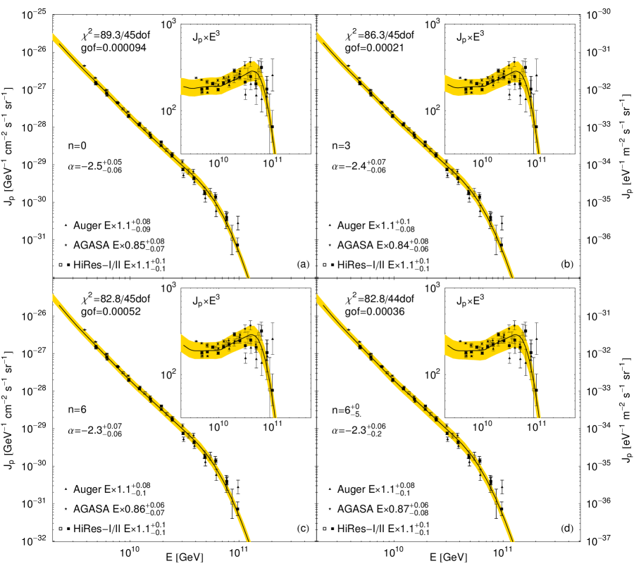
Figure 1: The flux of $J_{p}$ of ultra high energy cosmic rays that simultaneously fits Auger, HiRes-I and II, and AGASA data in the energy range $10^{9.6}$ GeV to $10^{11}$ GeV assuming a power-law injection spectrum with spectral index $\alpha$. Redshift evolution of the sources is parameterized by a power-law, $(1+z)^{n}$. The shaded bands and the quoted uncertainties are at the 2$\sigma$ C. L. and the error bars on the data points are 1$\sigma$ uncertainties. The energy scale of each experiment has been allowed to vary within the experiment’s energy scale uncertainty. The insets show $J_{p}E^{3}$ to facilitate comparison with other analyses.

The goodness of fit of these joint analyses is poor. This is primarily because the initial Auger data are noisy; see Tables 1 and 2. For now, we proceed to determine the corresponding cosmogenic neutrino fluxes.

	$\chi^{2}$	dof	gof
All data	86.3	45	$2.1\times 10^{-4}$
$-$Auger	37.6	32	0.23
$-$AGASA	58.8	32	$2.7\times 10^{-3}$
$-$HiRes	65.1	24	$1.2\times 10^{-5}$

Table 1: The $\chi^{2}$ for the number of degrees of freedom (dof) and the corresponding goodness of fit (gof) for analyses with $n=3$. The first row is for an analysis of all data. The cosmic ray spectrum is shown in the panel (b) of Fig. 1. Each subsequent row is the result with the indicated dataset removed from the analysis. Removal of the Auger data from the analysis improves the gof considerably.

	$\chi^{2}$	dof	gof
Auger	38.7	11	$6\times 10^{-5}$
AGASA	10.4	11	0.49
HiRes I+II	16.5	19	0.62

Table 2: Similar to Table 1, except that the results are for separate analyses of each experiment. The analysis of the Auger dataset yields a poor gof.

With the cosmic ray spectrum in hand we can compute the neutrino flux $J_{\nu}$ produced in the GZK chain by using Eq. (1) with $b=\nu$. The resulting cosmogenic neutrino fluxes (summed over flavors) are shown in Fig. 2. We do not show the case in which $n$ is free, since it fills the region between the $n=0$ and $n=6$ bands. Again, the bands correspond to the 2$\sigma$ C. L. The 95% C. L. model-independent upper bound obtained by the RICE collaboration from their latest data compilation is also shown.

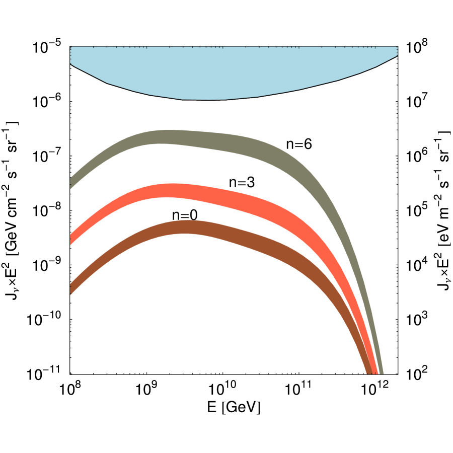
Figure 2: The 2$\sigma$ C. L. determinations of the cosmogenic neutrino flux (summed over all flavors) corresponding to the injection spectra of Fig. 1. The light shaded region is the 95% C. L. model-independent upper bound from RICE.

We have seen that a combined analysis including Auger data has an unsatisfactory goodness of fit even if super-GZK events seen by AGASA are excluded. This suggests that an alternative method to obtain the injection spectrum is called for.

The injection spectra obtained by unfolding are shown in Fig. 3. The widths of the bands are the 2$\sigma$ C. L. determinations. There are four different spectra since the unfolding was carried out experiment-by-experiment; we have not attempted an inversion of the joint data because there is too much freedom, rendering the results meaningless. So that a straightforward comparison can be made with the power-law injection case, we have analysed data in the energy range $10^{9.6}$ GeV to $10^{11}$ GeV; see panels (a) and (b) of Fig. 3. However, since the unfolding method is applicable even for super-GZK events, we have performed a separate analysis in which we include data up to $3\times 10^{11}$ GeV; see panels (c) and (d) of Fig. 3.

In the unfolding procedure it is assumed that there is no flux beyond the energy range spanned by the data. The sharp edges at the two ends of the spectra result because the spectra can not be extrapolated outside the energy interval. This is not true for the case in which a power-law injection spectrum is assumed. The bold line corresponds to a power law injection spectrum with spectral index $\alpha=-2.5$ in the $n=0$ plots and $\alpha=-2.3$ in the $n=6$ plots. The value of $\alpha$ is pinned-down by the statistically significant data at the lower end of the energy range. Thus, we have used the same spectral index in panels (a) and (c) and in panels (b) and (d). Note that the bold lines are extrapolated outside the range covered by the unfolding method. Results for values of $n$ between 0 and 6 are intermediate to those in the left-hand and right-hand panels of Fig. 3.

The neutrino spectra in Fig. 4 are obtained from Eq. (6). The bands correspond to the 2$\sigma$ C .L. The bold solid lines in the top and bottom panels are for power-law injection spectra with $E_{max}=10^{11}$ GeV and $E_{max}=3\times 10^{11}$ GeV, respectively. The bold dashed lines are the neutrino spectra of Fig. 2 and are provided for comparison. There we had set $E_{max}=3\times 10^{12}$ GeV. The agreement between the two methods is striking and provides support for the assumption that the injection spectrum has the form of a power-law. The poor fit obtained in the combined analysis with a power-law spectrum is likely due to systematic uncertainties that have not been accounted for.

Since the flux obtained from the unfolding procedure can be sizeable, it is essential to check that the accompanying cosmogenic photon flux is not in conflict with the EGRET observation of the diffuse gamma ray flux [30], as emphasized in Ref. [31]. We evaluated the photon flux using the publically available software, CRPropa [32], and find comfortable consistency with the EGRET bound. This is because the injection spectra we have found fall steeply with energy and because the largest value of $E_{max}$ we consider is $3\times 10^{11}$ GeV. As a consequence, the contribution to the photon flux measured by EGRET is tiny.

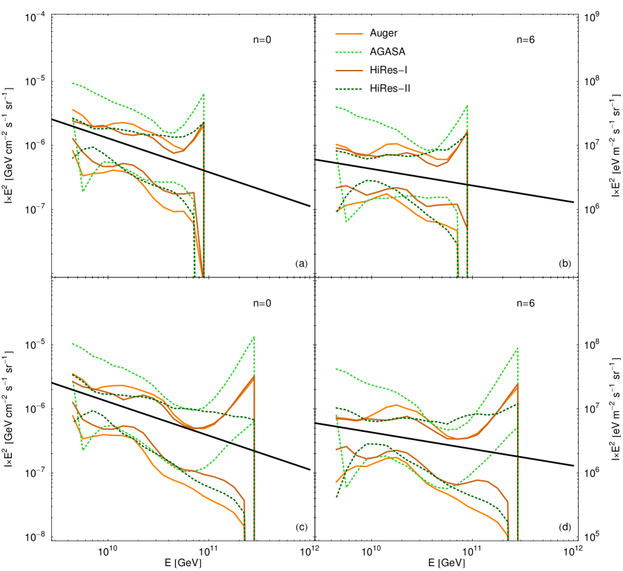
Figure 3: The 2$\sigma$ unfolded injection spectra from Auger, HiRes-I and II, and AGASA data. The upper (lower) two panels are for an analysis of data with energy between $10^{9.6}$ GeV to $10^{11}$ GeV ($10^{9.6}$ GeV to $3\times 10^{11}$ GeV). Redshift evolution of the sources is parameterized by a power-law, $(1+z)^{n}$. The bold line in the $n=0$ ($n=6$) plots is the injection spectrum of the form $E_{i}^{-2.5}$ ($E_{i}^{-2.3}$).

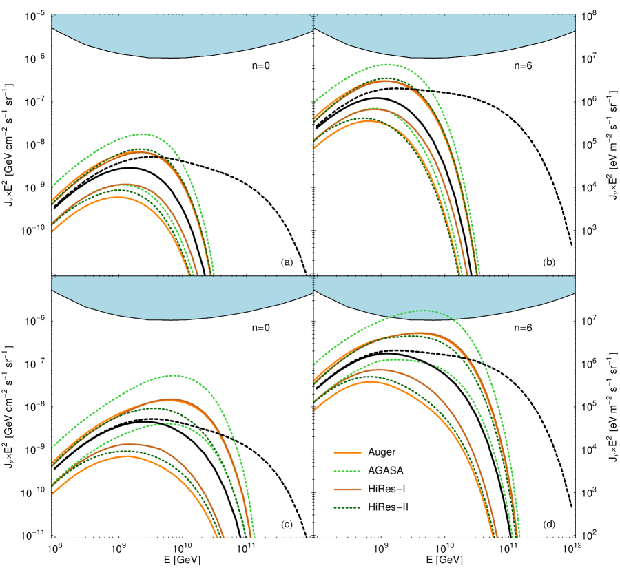
Figure 4: The 2$\sigma$ C. L. determinations of the total cosmogenic neutrino flux corresponding to the injection spectra of Fig. 3. The bold solid lines in the upper and lower panels are for power-law injection spectra with $E_{max}=10^{11}$ GeV and $E_{max}=3\times 10^{11}$ GeV, respectively. The agreement between the two methods is very good. The bold dashed lines are the neutrino spectra of Fig. 2, which were obtained for power-law injection spectra with $E_{max}=3\times 10^{12}$ GeV.

4 Constraints on the neutrino-nucleon cross section

In the energy range of interest ($10^{8}$ to $10^{11}$ GeV) the strongest bounds on the neutrino flux are those of the RICE experiment [33]. (The current bound from the ANITA experiment is stronger than that from RICE only above $10^{11}$ GeV [34]). The RICE bound is still much weaker than the determinations we made in the previous section. This allows us to place an upper bound on the neutrino-nucleon cross section; new physics can not increase the Standard Model cross section too much or high energy neutrinos would have been observed at neutrino telescopes. Note that if the upper limit of the cosmogenic neutrino flux from either method had been above the RICE limit, we could also have placed a constraint on the minimum required suppression of the cross section at ultra high energies.

The RICE collaboration has employed a method to obtain neutrino flux limits that are independent of specific neutrino flux models. See Appendix II of Ref. [33]. So long as new physics does not alter the energy dependence of the Standard Model cross section drastically (and only changes the overall normalization), we can constrain the neutrino-nucleon inelastic cross section by simply taking the ratio of the RICE bound to that of the lower bound of the cosmogenic neutrino flux.

Our 95% C.L. upper bound on the cross section (in units of the Standard Model cross section) is shown in Fig. 5 for $n=0$, 3 and 6. In each case, the colored curves correpond to the limit obtained by using the propagation inversion procedure and the black curve corresponds to a power-law injection spectrum. Bounds derived from RICE are valid only for $\sigma_{\nu}\mathrel{\raise 1.29167pt\hbox{$<$\kern-7.5pt\lower 4.30554pt\hbox{$\sim$}}}1$ mb [22]. Our cross section bounds are applicable only in the unshaded region.

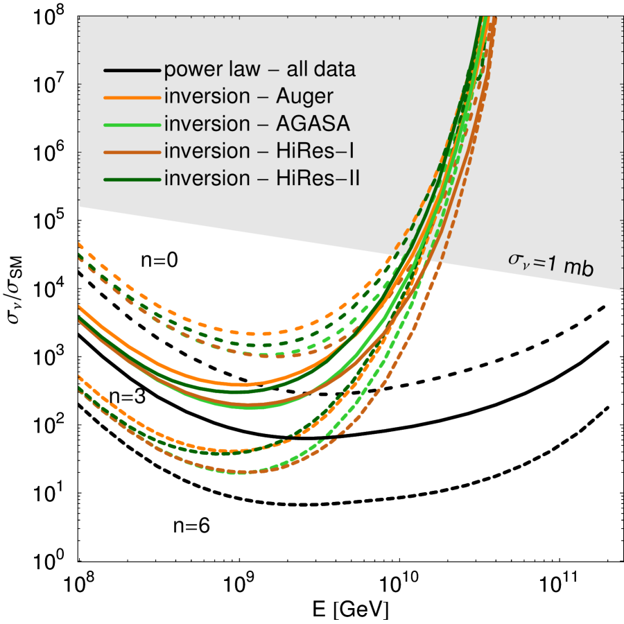
Figure 5: 95% C.L. upper bounds on the neutrino-nucleon cross section using our determinations of the cosmogenic neutrino flux and the model-independent flux limit from RICE. Our bounds are only valid in the unshaded region for which $\sigma_{\nu}<1$ mb.

5 Summary

We obtained the proton injection spectrum from cosmic ray data using two methods. In the first, we performed a combined analysis of HiRes-I and II, AGASA and Auger data in the energy interval, $10^{9.6}$ GeV to $10^{11}$ GeV, using a power law injection spectrum. We found the quality of the fit to be unsatisfactory even though we did not include super-GZK events in the analysis. The primary reason for the poor fit is apparently that the initial Auger data are noisy. In the second method, we implemented a regularized unfolding of the injection spectrum for each dataset separately.

We found the resultant cosmogenic neutrino flux using the injection spectra from both methods to be in excellent agreement with eachother. This suggests that the injection spectrum is well-modeled as a power-law and that the poor fit mentioned above is due to unaccounted-for systematic uncertainties.

Using the model-independent limit on the neutrino flux from RICE, we constrained the neutrino-nucleon cross section under the assumption that new physics modifies the charged-current and neutral-current interactions by the same constant factor.

Our results are succintly summarized in Figs. 1–5.

6 Acknowledgments

We thank S. Hussain and D. W. McKay for useful conversations and communications and D. Bergman for providing us with the latest HiRes data. We thank M. Ahlers and A. Ringwald for help with the use of their propagation matrices. Furthermore we acknowledge useful discussions with E. Armengaud, T. Beau and G. Sigl on the CRPropa software. This research was supported by the DOE under Grant No. DE-FG02-95ER40896, by the NSF under CAREER Award No. PHY-0544278 and Grant No. EPS-0236913, by the State of Kansas through the Kansas Technology Enterprise Corporation. Computations were performed on facilities supported by the NSF under Grants No. EIA-032078 (GLOW), PHY-0516857 (CMS Research Program subcontract from UCLA), and PHY-0533280 (DISUN), and by the University of Wisconsin Graduate School/Wisconsin Alumni Research Foundation.

Appendix A $\chi^{2}$ analysis

The observed flux $J_{i}^{O}$ is given by $n_{i}^{O}/\epsilon_{i}$, where $n_{i}^{O}$ and $\epsilon_{i}$ is the binned event rate and effective exposure, respectively, in bin $i$ of an experiment. The theoretically predicted flux $J_{i}^{t}$ is obtained from Eqs. (1,4). It depends on the overall normalization $\rho_{0}I_{0}$, the spectral index $\alpha$ and on redshift evolution as parameterized by $n$. The theoretical event rate $n_{i}^{t}$ is related to the theoretical flux by $n_{i}^{t}=J_{i}^{t}\epsilon_{i}$.

In order to incorporate the effect of the energy scale uncertainty on the event rates, we replace the (observed) energy $E_{i}$ by $(1+\gamma)E_{i}$, where $\gamma$ is the fractional energy scale uncertainty of the experiment. The details follow the implementation in GLoBES [35]. Thus, the theoretical flux becomes a function of $\rho_{0}I_{0},\alpha,n$ and 3 $\gamma$’s.

Since the the observed event rate can be very low or even zero, we use the Poissonian $\chi^{2}$-function (see, e.g. [36]),

$$\chi^{2}(n_{i}^{O},n_{i}^{t})=2\sum_{i=1}^{N}\left(n_{i}^{t}-n_{i}^{O}+n_{i}^{O}\log\frac{n_{i}^{O}}{n_{i}^{t}}\right)\,.$$ (7)

It is crucial to propagate the errors and their correlations consistently as we are interested in both, the proton flux and the derived cosmogenic neutrino flux. The supposition that the errors are uncorrelated would lead to an incorrect result. The allowed region at confidence level $CL$ is defined by requiring that $\Delta\chi^{2}\leq\chi^{2}_{CL}$, where $\chi^{2}_{CL}$ is given by the $CL^{th}$ percentile of the $\chi^{2}$-distribution after accounting for the 5 or 6 free parameters in the analysis. We use a Markov Chain Monte Carlo (MCMC) method [37] based on the Metropolis-Hastings algorithm. Specific care has to be taken to ensure that the chain has reached equilibrium, i.e., its asymptotic state. We employ the convergence diagnostic of Ref. [38] since it is conceptionally simple and does not incur a large computational burden.

Appendix B Unfolding procedure

The propagation of ultra high energy cosmic rays is described by Eq. (1) which is a Fredholm equation of the first kind. The authors of Ref. [20] have attempted to infer $I(E_{i})$ from the observed flux $J_{b}(E)$ and $G_{b}(E,E_{i})$ via direct inversion. Unfortunately, the problem is ill posed unless regularized unfolding is carried out; see Ref. [39] for a detailed exposition. An illustration of this fact is provided in Fig. 6.

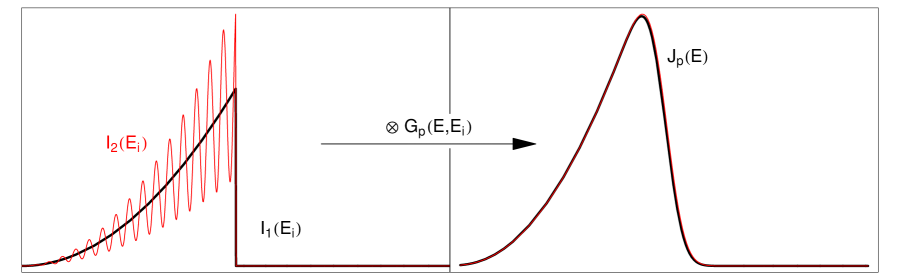
Figure 6: Two different injection spectra, $I_{1}(E_{i})$ and $I_{2}(E_{i})$, that yield the same cosmic ray spectrum $J_{p}(E)$ on folding in $G_{p}(E,E_{i})$. A naive unfolding of data corresponding to $J_{p}(E)$ (i.e., with random fluctuations included) could result in a highly oscillatory injection spectrum like $I_{2}(E_{i})$ which may be not be positive definite at all energies. The goal of regularized unfolding is to extract the smooth spectrum $I_{1}(E_{i})$ with the minimal introduction of bias.

We follow Tikhonov regularization described in Ref. [40]. The $\chi^{2}$ definition of Eq. (7) must be modified to include a regularization function $S(\mathbf{n}^{t})$ and a regularization parameter $\beta$,

$$\chi^{2}(\mathbf{n}^{t})+\beta S(\mathbf{n}^{t})\,,$$ (8)

with the understanding that the $n^{t}_{i}$ are the parameters in the fit; i.e., the $n^{t}_{i}$ are not derived from a model. It can be shown that $\chi^{2}$-minimization with $\beta=0$ is an unbiased estimator with the smallest variance but which yields highly oscillatory solutions. One the other hand, the $\beta\rightarrow\infty$ case yields a maximally smooth estimator with vanishing variance and a clear bias (since the result no longer depends on the data). The parameter $\beta$ determines the relative weight placed on the data in comparison to the degree of smoothness of the solution. In a Bayesian spirit this is equivalent to assuming a prior which favors smooth solutions with $\beta$ controlling the width of the prior. The smaller $\beta$ is, the less impact the prior will have and vice versa.

It remains to choose $S(\mathbf{n}^{t})$ (to obtain a smooth solution) and $\beta$ (to define the trade-off between bias and variance). For our application, the mean square of the second derivative

$$S(\mathbf{\mathbf{n}^{t}})=-\sum_{i=1}^{N-2}\left(-n_{i}^{t}+2n_{i+1}^{t}-n_{i+2}^{t}\right)^{2}\,,$$ (9)

works very well.

Our criteria for obtaining $\beta$ are that injection spectrum be positive definite and that the overall $\chi^{2}$ for an individual dataset not increase by more than 50% relative to that obtained from the power-law fit. Values of $\beta$ above unity satisfy the former requirement, while $\beta$ needs to be less than 10 to satisfy the latter. We select $\beta=5$ for all four datasets, which adequately suppresses any spurious oscillations.

We estimate the variance of the result by generating 1000 random realizations of the data sets by assuming a Poisson distribution in each bin with a mean value $n_{i}^{O}$. For each of these random realizations we repeat the above procedure and construct the covariance matrix $\mathbf{C}$ which is then used to obtain upper and lower bounds on the proton and neutrino fluxes by retaining only those realizations which satisfy

$$\mathbf{n}^{t}\mathbf{C}^{-1}(\mathbf{n}^{t})^{T}\leq\chi^{2}_{CL}\,.$$ (10)

Here, $\chi^{2}_{CL}$ is given by the $CL^{th}$ percentile of the values obtained for the left hand side.

References

- [1] H. Aoyama and H. Goldberg, Phys. Lett. B 188, 506 (1987); A. Ringwald, Nucl. Phys. B 330, 1 (1990); O. Espinosa, Nucl. Phys. B 343, 310 (1990); V. V. Khoze and A. Ringwald, Phys. Lett. B 259, 106 (1991).
- [2] P. C. Argyres, S. Dimopoulos and J. March-Russell, Phys. Lett. B 441, 96 (1998) [arXiv:hep-th/9808138]; T. Banks and W. Fischler, arXiv:hep-th/9906038.
- [3] S. Nussinov and R. Shrock, Phys. Rev. D 59, 105002 (1999) [arXiv:hep-ph/9811323]; P. Jain, D. W. McKay, S. Panda and J. P. Ralston, Phys. Lett. B 484, 267 (2000) [arXiv:hep-ph/0001031].
- [4] N. Arkani-Hamed, S. Dimopoulos and G. R. Dvali, Phys. Lett. B 429, 263 (1998) [arXiv:hep-ph/9803315]; Phys. Rev. D 59, 086004 (1999) [arXiv:hep-ph/9807344]; I. Antoniadis, N. Arkani-Hamed, S. Dimopoulos and G. R. Dvali, Phys. Lett. B 436, 257 (1998) [arXiv:hep-ph/9804398].
- [5] G. Domokos and S. Kovesi-Domokos, Phys. Rev. Lett. 82, 1366 (1999) [arXiv:hep-ph/9812260]. F. Cornet, J. I. Illana and M. Masip, Phys. Rev. Lett. 86, 4235 (2001) [arXiv:hep-ph/0102065].
- [6] M. Ribordy et al. [IceCube Collaboration], arXiv:astro-ph/0509322.
- [7] D. J. Bird et al. [HIRES Collaboration], Phys. Rev. Lett. 71, 3401 (1993);
- [8] K. Greisen, Phys. Rev. Lett. 16, 748 (1966); G. T. Zatsepin and V. A. Kuzmin, JETP Lett. 4, 78 (1966) [Pisma Zh. Eksp. Teor. Fiz. 4, 114 (1966)].
- [9] V. S. Beresinsky and G. T. Zatsepin, Phys. Lett. B 28, 423 (1969); Yad. Fiz. 11, 200 (1970); F. W. Stecker, Astrophys. J. 228, 919 (1979).
- [10] F. W. Stecker, Phys. Rev. Lett. 21, 1016 (1968); F. A. Aharonian and J. W. Cronin, Phys. Rev. D 50, 1892 (1994); J. W. Elbert and P. Sommers, Astrophys. J. 441, 151 (1995) [arXiv:astro-ph/9410069].
- [11] S. Yoshida and M. Teshima, Prog. Theor. Phys. 89, 833 (1993);
- [12] T. K. Gaisser et al. [HIRES Collaboration], Phys. Rev. D 47, 1919 (1993); D. J. Bird et al., Astrophys. J. 424, 491 (1994); G. C. Archbold, Ph.D. Thesis, University of Utah, UMI-30-54514; T. Abu-Zayyad et al. [High Resolution Fly’s Eye Collaboration], Astropart. Phys. 23, 157 (2005) [arXiv:astro-ph/0208301].
- [13] D. R. Bergman, poster at 29th International Cosmic Ray Conference, Pune, India, 2005, and private communication.
- [14] M. Takeda et al., Phys. Rev. Lett. 81, 1163 (1998) [arXiv:astro-ph/9807193]. S. Yoshida et al. [AGASA Collaboration], in Proceedings of 27th International Cosmic Ray Conference, Hamburg, Germany, 2001, Vol. 3, pg. 1142; http://www-akeno.icrr.u-tokyo.ac.jp/AGASA/ (June 24, 2003).
- [15] M. Takeda et al., Astropart. Phys. 19, 447 (2003) [arXiv:astro-ph/0209422].
- [16] A. Etchegoyen [Pierre Auger Collaboration], Astrophys. Space Sci. 290, 379 (2004); K. S. Capelle, J. W. Cronin, G. Parente and E. Zas, Astropart. Phys. 8, 321 (1998) [arXiv:astro-ph/9801313].
- [17] R. J. Protheroe and P. A. Johnson, Astropart. Phys. 4, 253 (1996) [arXiv:astro-ph/9506119].
- [18] S. Yoshida, H. y. Dai, C. C. H. Jui and P. Sommers, Astrophys. J. 479, 547 (1997) [arXiv:astro-ph/9608186]; R. Engel, D. Seckel and T. Stanev, Phys. Rev. D 64, 093010 (2001) [arXiv:astro-ph/0101216]; O. E. Kalashev, V. A. Kuzmin, D. V. Semikoz and G. Sigl, Phys. Rev. D 66, 063004 (2002) [arXiv:hep-ph/0205050].
- [19] D. R. Bergman [The HiRes Collaboration], Nucl. Phys. Proc. Suppl. 136, 40 (2004) [arXiv:astro-ph/0407244].
- [20] Z. Fodor, S. D. Katz, A. Ringwald and H. Tu, JCAP 0311, 015 (2003) [arXiv:hep-ph/0309171].
- [21] M. Ahlers, L. A. Anchordoqui, H. Goldberg, F. Halzen, A. Ringwald and T. J. Weiler, Phys. Rev. D 72, 023001 (2005) [arXiv:astro-ph/0503229].
- [22] L. A. Anchordoqui, Z. Fodor, S. D. Katz, A. Ringwald and H. Tu, JCAP 0506, 013 (2005) [arXiv:hep-ph/0410136].
- [23] J. N. Bahcall and E. Waxman, Phys. Lett. B 556, 1 (2003) [arXiv:hep-ph/0206217]; D. De Marco, P. Blasi and A. V. Olinto, Astropart. Phys. 20, 53 (2003) [arXiv:astro-ph/0301497].
- [24] D. R. Bergman, in Proceedings of 29th International Cosmic Ray Conference, Pune, India, 2005.
- [25] P. Sommers [Pierre Auger Collaboration], arXiv:astro-ph/0507150.
- [26] V. Berezinsky, A. Z. Gazizov and S. I. Grigorieva, arXiv:hep-ph/0204357.
- [27] M. Nagano et al., J. Phys. G 18, 423 (1992); T. Abu-Zayyad et al. [HiRes-MIA Collaboration], Astrophys. J. 557, 686 (2001) [arXiv:astro-ph/0010652].
- [28] Z. Fodor and S. D. Katz, Phys. Rev. D 63, 023002 (2001) [arXiv:hep-ph/0007158]; Z. Fodor, S. D. Katz, A. Ringwald and H. Tu, Phys. Lett. B 561, 191 (2003) [arXiv:hep-ph/0303080].
- [29] http://www.desy.de/~uhecr/propagation.html
- [30] A. W. Strong, I. V. Moskalenko and O. Reimer, arXiv:astro-ph/0306345; P. Sreekumar et al. [EGRET Collaboration], Astrophys. J. 494, 523 (1998) [arXiv:astro-ph/9709257].
- [31] D. V. Semikoz and G. Sigl, JCAP 0404, 003 (2004) [arXiv:hep-ph/0309328].
- [32] E. Armengaud, G. Sigl, T. Beau and F. Miniati, arXiv:astro-ph/0603675.
- [33] I. Kravchenko et al., Phys. Rev. D 73, 082002 (2006) [arXiv:astro-ph/0601148].
- [34] S. W. Barwick et al. [ANITA Collaboration], Phys. Rev. Lett. 96, 171101 (2006) [arXiv:astro-ph/0512265].
- [35] P. Huber, M. Lindner, and W. Winter, Comput. Phys. Commun. 167, 195 (2005), hep-ph/0407333.
- [36] D. E. Groom et al., Eur. Phys. J. C15, 1 (2000).
- [37] C. Andrieu, N. de Freitas, A. Doucet, and M. Jordan, Machine Learning 50, 5 (2003).
- [38] J. Dunkley, M. Bucher, P. G. Ferreira, K. Moodley, and C. Skordis, Mon. Not. Roy. Astron. Soc. 356, 925 (2005), astro-ph/0405462.
- [39] I. J. D. Craig and J. C. Brown, Inverse Problems in Astronomy: a guide to inversion strategies for remotely sensed data (Adam Hilger Ltd, 1986).
- [40] G. Cowan, Statistical Data Analysis, (Oxford University Press, 1998).