CERN-PH-TH/2006-119 Axion alternatives

Abstract

If recent results of the PVLAS collaboration proved to be correct, some alternative to the traditional axion models are needed. We present one of the simplest possible modifications of axion paradigm, which explains the results of PVLAS experiment, while avoiding all the astrophysical and cosmological restrictions. We also mention other possible models that possess similar effects.

1 Introduction

It has been understood long ago, that the presence of light pseudoscalar particles, with coupling to the electromagnetic field of the form

$$\mathcal{L}_{\textsc{em}+\phi}=-\frac{1}{4}F_{\mu\nu}^{2}+\frac{1}{2}(\partial_{\mu}\phi)^{2}-\frac{m^{2}_{\phi}}{2}\phi^{2}-\frac{1}{4f_{\phi}}\phi\,\epsilon^{\mu\nu\lambda\rho}F_{\mu\nu}F_{\lambda\rho}\;,$$ (1)

leads to a number of signature effects [1, 2, 3, 4, 5, 6]. In particular, in external magnetic field, vacuum becomes birefringent and dichroic. These effects (change of linear polarization into the elliptic one and rotation of the polarization plane of linearly polarized light) can be qualitatively understood as follows. Interaction (1) leads to an effective mass for the component of the photon, polarized along the direction of the external magnetic field (see Fig.-479), while perpendicularly polarized component remains massless. Recently, PVLAS collaboration reported observation of such an effect of rotation of polarization [7].

However, the axion interpretation of the PVLAS data comes in contradiction with other experimental constraints (see e.g. [8]). Namely, PVLAS data can be interpreted in terms of axion-like particle (ALP) with Lagrangian (1) if one identifies

$$m_{\phi}=1-1.5\;\mathrm{meV};\qquad f_{\phi}=(2-6)\times 10^{5}~{}\text{GeV}$$ (2)

These numbers disagree, however, with both astrophysical bounds (see e.g. [9])

$$f_{a,\,\mathrm{stellar}}\gtrsim 10^{10}~{}\text{GeV}$$ (3)

and the results of CAST collaboration [10], which tries to detect the flux of $\phi$ coming from the Sun and its conversion into photons in a strong magnetic field. Absence of such a signal puts a lower bound on $f_{\phi}$, compatible with (3):

$$f_{\phi}>8.6\times 10^{9}~{}\text{GeV}\quad\text{for}\quad m_{\phi}\lesssim 0.02~{}\text{eV}$$ (4)

Clearly, there exists a strong contradiction between the results of PVLAS and limits (3)–(4), which implies that the simple axion model (1) should be modified. Attempts to avoid the astrophysical constraints (3)–(4) have been discussed in the literature (see e.g. [11, 12, 13]). We note that models with ALPs are historically motivated by the CP problem in QCD and the Peccei-Quinn mechanism of its solution [14, 15]. Therefore the attempts to avoid stellar constraints are usually based on modification of the axion Lagrangian, making the theory more sophisticated.

In this work we suggest a different way to reconcile the results of PVLAS experiment (2) with the constraints (3)–(4). We present another very simple model which provides almost the same properties of propagation of photons in the magnetic field as models with axion. This model is not inspired by the strong CP problem and has rather different particle physics motivation. We show that in such a model there is no contradiction between PVLAS data interpreted as a mass of photon in the magnetic field and astrophysical and CAST constraints. At the end we briefly discuss high-energy motivation of this model, various modifications of the effective theory coming from different fundamental theories and possibilities to distinguish experimentally between them. We plan to discuss these issues in detail elsewhere [16].

The plan of the paper is the following. In the section 2 we describe the effect of an effective photon mass generation in a magnetic field and present the model. In the section 3 we calculate the propagator of of the photon in a magnetic field in our model. Finally, in the last section 4, we shortly discuss our results, possible theoretical origin of our model and its future developments.

Figure -479: Diagram for effective mass of a photon in the external magnetic field $H$. The dashed line corresponds to an exchange of the hypothetical new particle.

2 New vector boson

The effects of birefringence and dichroism can be qualitatively described as generation of the effective mass of the photon via the process, shown on Fig. -479. Qualitatively, one expects this magnetic mass to behave as

$$m_{\gamma,H}\sim\frac{\bm{\kappa}H}{m_{\textsc{alp}}}$$ (5)

where $m_{\textsc{alp}}$ is the mass of intermediate particle (whose propagator is denoted by dashed line on Fig. -479) and $\bm{\kappa}$ is a dimensionless coupling constant in the vertex defining the interaction of photon with this intermediate particle in a constant magnetic field. On the other hand, both constraints (3) and (4) stem from production (annihilation) of real ALPs, i.e. from processes of the type shown in Fig. -478. By choosing $\bm{\kappa}$ to be very small one can arbitrarily suppress them and still have the effect (5) preserved, provided that $m_{\textsc{alp}}$ also goes to zero with $\bm{\kappa}\to 0$.

One of the simplest theories with this property is the theory of a gauge boson $B$ acquiring mass from a Higgs field $m_{B}=\bm{\kappa}v_{B}$ with $\bm{\kappa}$ being its corresponding charge. Then, one could have an interaction with the photon $A$ via the Chern-Simons-like term

$$\mathcal{L}_{\textsc{cs}}=\bm{\kappa}\,\epsilon^{\mu\nu\lambda\rho}A_{\mu}B_{\nu}(\partial_{\lambda}A_{\rho})$$ (6)

We will see in a moment that the appearance of the same charge $\bm{\kappa}$ in front of this interaction is natural and is dictated by gauge invariance. Clearly, the term (6) is the close cousin of the axion-like interaction (1), which is easy to see if one substitutes $B_{\mu}$ by $\partial_{\mu}\phi$. However, the full theories are not equivalent as we will show below.

Naively, the theory with the interaction (6) is not gauge invariant, its A-gauge variation being proportional to $F_{A}\tilde{}F_{B}$, (where by tilde we denote dual field-strengths). This can, however, be amended and the simplest theory which possesses the interaction (6) and is gauge invariant is the following:

$$\mathcal{L} =-\frac{1}{4}|F_{A}|^{2}-\frac{1}{4}|F_{B}|^{2}+\frac{v_{\gamma}^{2}}{2}(D_{\mu}\theta_{1})^{2}+\frac{v_{B}^{2}}{2}(D_{\mu}\theta_{2})^{2}$$ (7)

$$\hphantom{=}+\theta_{1}\epsilon^{\mu\nu\lambda\rho}(F_{A})_{\mu\nu}(F_{B})_{\lambda\rho}+\theta_{2}\epsilon^{\mu\nu\lambda\rho}(F_{A})_{\mu\nu}(F_{A})_{\lambda\rho}-2\bm{\kappa}\,\epsilon^{\mu\nu\lambda\rho}A_{\mu}B_{\nu}(F_{A})_{\lambda\rho}$$

where

$$D_{\mu}\theta_{1}=\partial_{\mu}\theta_{1}+\bm{\kappa}A_{\mu};\quad D_{\mu}\theta_{2}=\partial_{\mu}\theta_{2}-\bm{\kappa}B_{\mu}$$ (8)

The theory (7) may seem somewhat ad hoc. However, such interactions appear generically in effective theories of models with chiral fermions, which acquire mass via Yukawa couplings with the charged Higgs fields [17, 18]. We will comment on the possible microscopic origin of the theory (7) in the Discussion section, the detailed analysis will appear elsewhere [16]. The fields $\theta_{1}$ and $\theta_{2}$ are the phases of the Higgs fields, which provide masses to both gauge fields. The coefficients in Eq. (7) are fixed by requirement of gauge invariance with respect to the two $\mathrm{U}(1)$ groups: $\mathrm{U}(1)_{\textsc{em}}\times\mathrm{U}(1)_{B}$:

$$\mathrm{U}(1)_{\textsc{em}}: \delta_{\lambda}\theta_{1} =-\bm{\kappa}\lambda; \delta_{\lambda}A_{\mu}=\partial_{\mu}\lambda$$ (9)

$$\mathrm{U}(1)_{B}: \delta_{\beta}\theta_{2} =\bm{\kappa}\beta; \delta_{\lambda}B_{\mu}=\partial_{\mu}\beta$$ (10)

where only non-trivial gauge-variations are shown for each group. The same theory, considered in the unitary gauge for both fields, reads:

$$\mathcal{L}=-\frac{1}{4}|F_{A}|^{2}-\frac{1}{4}|F_{B}|^{2}+\frac{m_{\gamma}^{2}}{2}A_{\mu}^{2}+\frac{m_{B}^{2}}{2}B_{\mu}^{2}-2\bm{\kappa}\epsilon^{\mu\nu\lambda\rho}A_{\mu}B_{\nu}(F_{A})_{\lambda\rho}$$ (11)

where

$$m_{\gamma}=\bm{\kappa}v_{\gamma};\qquad m_{B}=\bm{\kappa}v_{B}$$ (12)

Figure -478: Creation of $B_{\mu}$ in the external fields

The theory (11) will be analyzed in details in the next Section. However, one can anticipate the results. Substituting uniform magnetic field $H$ in place of $F_{A}$ in the interaction term (11) and diagonalizing the quadratic part of the Lagrangian, one can see that the mass of the photon shifts: $m_{\gamma}^{2}\to m_{\gamma}^{2}+H^{2}/v_{B}^{2}$, the dependence of $\bm{\kappa}$ cancels out and the effect is not suppressed in the limit of small $\bm{\kappa}$. This allows us to choose $v_{B}\sim 10^{5}~{}\text{GeV}$ in order to explain the PVLAS data and choose $\bm{\kappa}\lll 1$ to suppress emission of $B$-boson from stars. Actually, by looking at Eqs. (11)–(12), it is clear that $\bm{\kappa}$ should be very small. Indeed, according to the Particle Data Group [19] the upper bound on photon mass is

$$m_{\gamma,\textsc{pdg}}<6\times 10^{-17}~{}\text{eV}\;.$$ (13)

We will choose the constant $\bm{\kappa}$ in such a way, as to ensure the limit (13) as well as the suppression of $B$ production in stars and in the early Universe.

3 Propagator of light in a uniform magnetic field

In this Section we compute the propagator of photon in the model of Section 2 and show that it leads indeed to effects of birefringence and dichroism.

In the theory (11) the full propagator of a photon $G_{\mu\nu}$ can be determined from the following equation:

$$G^{-1}_{\mu\nu}=(G^{0})^{-1}_{\mu\nu}-\Pi_{\mu\nu}(k)$$ (14)

where the 1PI self-energy of the photon $\Pi_{\mu\nu}$ is determined by the diagram -479, and the tree level propagators of the $B$-field and the photon are given by

$$D_{\mu\nu}(k)=\frac{\eta_{\mu\nu}-{k_{\mu}k_{\nu}}/{m_{B}^{2}}}{k^{2}-m_{B}^{2}+i\epsilon};\qquad G^{0}_{\mu\nu}=\frac{\eta_{\mu\nu}-{k_{\mu}k_{\nu}}/{m_{\gamma}^{2}}}{k^{2}-m_{\gamma}^{2}+i\epsilon}\,.$$ (15)

$(G^{0})^{-1}_{\hphantom{-1}\mu\nu}$ is the inverse propagator (15):

$$(G^{0})^{-1}_{\mu\nu}=(k^{2}-m_{\gamma}^{2})\eta_{\mu\nu}-{k_{\mu}k_{\nu}}$$ (16)

We are interested in the propagation of light in the uniform magnetic field $H=F_{23}$. Then, $\Pi_{\mu\nu}$ is given by

$$\Pi^{ab}=\bm{\kappa}^{2}H^{2}\epsilon^{ac}\epsilon^{bd}\left(\frac{\eta_{cd}-{k_{c}k_{d}}/{m_{B}^{2}}}{k^{2}-m_{B}^{2}+i\epsilon}\right);\qquad\Pi_{ab}=\eta_{aa^{\prime}}\eta_{bb^{\prime}}\Pi^{a^{\prime}b^{\prime}}$$ (17)

with all other components equal to zero. One can rewrite $\Pi_{ab}$ as

$$\Pi_{ab}=-\frac{\bm{\kappa}^{2}H^{2}}{m_{B}^{2}(k^{2}-m_{B}^{2})}\begin{pmatrix}k_{x}^{2}+m_{B}^{2}&k_{x}\omega\\ k_{x}\omega&\omega^{2}-m_{B}^{2}\end{pmatrix}_{ab}$$ (18)

3.1 Photon propagating perpendicularly to the magnetic field

Let us consider the case when a photon is propagating along the $z$ axis with the magnetic field pointing in $x$ direction. We have:

$$\Pi_{ab}=-\frac{\bm{\kappa}^{2}H^{2}}{k^{2}-m_{B}^{2}}\eta_{ab}-\frac{\bm{\kappa}^{2}H^{2}}{m_{B}^{2}(k^{2}-m_{B}^{2})}\begin{pmatrix}0&0\\ 0&\omega^{2}\end{pmatrix}$$ (19)

and one can find explicitly the propagator $G_{\mu\nu}$. A straightforward computation shows that in this case the $\{x,y\}$ block of the matrix $G_{\mu\nu}$ is diagonal and therefore the components $A_{x}$ and $A_{y}$ are determined by $G_{xx}$ and $G_{yy}$ correspondingly. It is then easy to see that the propagator $G_{xx}$ (describing wave with the electric field along the magnetic field $H$) changes, while $G_{yy}$ (polarization, orthogonal to the magnetic field) remains unchanged! Namely, $G_{xx}$ is given by

$$G_{xx}(\omega,k_{z})=-\frac{(k^{2}-m_{B}^{2})}{(k^{2}-m_{\gamma}^{2}+i\epsilon)(k^{2}-m_{B}^{2}+i\epsilon)+\frac{\bm{\kappa}^{2}H^{2}}{m_{B}^{2}}(m_{B}^{2}-\omega^{2})}\;,$$ (20)

where $k^{2}=\omega^{2}-k_{z}^{2}$.

The zeros of the denominator are given by the following equation:

$$(k^{2}-m_{\gamma}^{2})(k^{2}-m_{B}^{2})+\frac{H^{2}}{v_{B}^{2}}(m_{B}^{2}-\omega^{2})=0$$ (21)

(where we have used $m_{B}=\bm{\kappa}v_{B}$). This equation describes two propagating modes, one with a mass close to that of the photon:

$$\omega_{\gamma}^{2}(k_{z})\simeq k_{z}^{2}(1-\eta)+m_{\gamma}^{2}+\eta m_{B}^{2}\\$$ (22)

and another with a mass, close to that of $B$ boson

$$\omega_{B}^{2}(k_{z})\simeq k_{z}^{2}(1+\eta)+m_{B}^{2}$$ (23)

Both solutions are found in the leading approximation in $(H/v_{B}^{2})$ and $(m_{\gamma}/m_{B})$ and we have introduced a small parameter $\eta={H^{2}}/{v_{B}^{4}}$. Substituting these modes into the propagator (20), we see that the admixture of the “heavy mode” (23) is suppressed by the small parameter $\eta$ and in the first approximation we obtain the photon propagating with the mass

$$m_{\gamma,H}^{2}\simeq\frac{H^{2}}{v_{B}^{2}}$$ (24)

Let us compare the result (20)–(21) with the similar “secular equation” of Ref. [5]:

$$k^{2}(k^{2}-m_{\phi}^{2})-\frac{H^{2}}{f_{\phi}^{2}}\omega^{2}=0$$ (25)

We see that there is a trivial difference due to $m_{\gamma}$ and $(\omega^{2}-m_{B}^{2})$ instead of $\omega^{2}$ in the last term of Eq. (21). However, we expect $\omega\gg m_{B}$ (in experiments $\omega\sim 1~{}\text{eV}$). Therefore, the effects for a photon, propagating in a perpendicular magnetic field, remain in our model the same as in the model with the axion if one identifies

$$f_{\phi}\to v_{B};\qquad m_{\phi}\to m_{B}$$ (26)

Using the PVLAS values for these constants we obtain:

$$m_{B}\sim 10^{-3}~{}\text{eV};\qquad v_{B}\sim 10^{5}~{}\text{GeV};\qquad\bm{\kappa}\sim 10^{-17};\quad v_{\gamma}\sim\frac{m_{\gamma}}{\bm{\kappa}}\lesssim 1~{}\text{eV}$$ (27)

The exchange by this new light boson leads in principle to corrections on the gravitational attraction of two bodies. The mass and coupling constant (27) are compatible with the existing constraints from the searches of such a “fifth force” with a range smaller than $0.1$ cm (in our case $m_{B}^{-1}\sim 0.01$ cm) (see e.g. [24]).

4 Discussion

In this work we proposed a simple alternative to the axion model, which reproduces the effects of rotation of the polarization plane, recently observed by PVLAS collaboration, and avoids the constraints coming from astrophysical and cosmological data. This low-energy theory predicts the existence of a new light vector field (rather than a pseudoscalar particle), which interacts with the photon via Chern-Simons-like terms. Such terms generically appear as effective interactions in theories with chiral fermions due to fermionic loop effects [17, 18]. The structure of interactions in Lagrangians similar to (7) is dictated by the requirement of anomaly cancellation and the coefficients ($\bm{\kappa}$ in our case) are uniquely fixed. For example, such terms would appear in the model with fermions charged as shown in Table 1.

	$\phi_{1}$	$\phi_{2}$	$\psi_{L}$	$\psi_{R}$	$\psi_{L}^{\prime}$	$\psi_{R}^{\prime}$	$\chi_{L}$	$\chi_{R}$	$\chi_{L}^{\prime}$	$\chi_{R}^{\prime}$
$\mathrm{U}(1)_{\gamma}{}$	$\bm{\kappa}{}$	$0$	$q_{1}$	$q_{1}+\bm{\kappa}{}$	$q_{1}+\bm{\kappa}{}$	$q_{1}$	$q_{2}$	$q_{2}$	$q_{2}^{\prime}$	$q_{2}^{\prime}$
$\mathrm{U}(1)_{B}$	$0$	$-\bm{\kappa}{}$	$\beta_{1}$	$\beta_{1}$	$\beta_{1}^{\prime}$	$\beta_{1}^{\prime}$	$\beta_{2}$	$\beta_{2}-\bm{\kappa}{}$	$\beta_{2}-\bm{\kappa}{}$	$\beta_{2}$

Table 1: A simple choice of charges of fermions and Higgs fields, which leads to the low-energy effective action (7). Potential for Higgs fields ensure that $\phi_{1}=v_{\gamma}e^{i\theta_{1}}$ and $\phi_{2}=v_{B}e^{i\theta_{2}}$. The charges are chosen such that there are no $\gamma^{3}$ and $B^{3}$ triangle anomalies for both groups of fermions $\psi$ and $\chi$. On the other hand, mixed anomalies cancel between the two groups of fermions. Masses of $\psi$-fermions are generated via Yukawa interaction with the Higgs field $\phi_{1}$ and masses of $\chi$-fermions by the Higgs field $\phi_{2}$.

Clearly, for such a model to become realistic, one needs to implement it in an extension of the Standard Model (SM). The realization of the model (7) as an effective theory derived from a consistent extension of the SM will be reported separately [16]. We would like to mention here that, apart from integrating out four-dimensional fermions à la D’Hoker and Fahri [17, 18], axionic and Chern-Simons terms can also appear from higher-dimensional theories. For example, such effective theories generically appear in realizations of SM on D-branes in string theory [25].

In this work, we presented the simplest example of appearance of axion-like interactions as a consequence of cancellation of gauge anomalies between various sectors of the theory. Physically, this is a different approach to the building of such models, as compared to the more conventional axions related to the strong CP problem. Other models of this kind can appear in various realistic scenarios, which will also be discussed in [16].

There exists another class of theories, where effects, similar to those discussed in this paper, may appear. In theories with extra dimensions anomaly cancellation may occur between light particles, living in 4 dimensions and very heavy particles, propagating in the higher-dimensional space (the so called anomaly inflow mechanism [26, 27]). The low-energy limit of such a theory may not have a description in terms of a local 4-dimensional effective theory. The mechanism of anomaly inflow is realized in nature in the case of quantum Hall effect [28, 29] where the 2-dimensional anomaly of the edge excitations of the quantum Hall droplet is canceled by the inflow from a 3-dimensional Chern-Simons term. A 4-dimensional example of such a theory was considered in [30, 31]. It was shown that the anomaly cancellation between a 4-dimensional SM-like theory and a 5-dimensional bulk theory may lead to an effect similar to (5), i.e. appearance of a mass for the photon in the presence of strong magnetic field. The key difference between the effect described in [30, 31] and the effects considered in this work is the dependence of the mass on the magnetic field. Namely, this dependence had the form

$$m_{\gamma,H}\sim\sqrt{\alpha_{\textsc{em}}\kappa_{0}H}$$ (28)

where $\alpha_{\textsc{em}}$ is the fine-structure constant and $\kappa_{0}$ is a dimensionless constant, characterizing the deviation of the charges of light fermions from their anomaly-free values (similar to $\bm{\kappa}$ of our model). Numerically, this effect is consistent with PVLAS data. The different from (5) dependence of the induced photon mass on the magnetic field can thus serve as a peculiar signature of the presence of extra dimensions. Thus, the measurement of the magnetic field dependence of the effects of birefringence and dichroism can distinguish between various models of “physics beyond the Standard Model”.

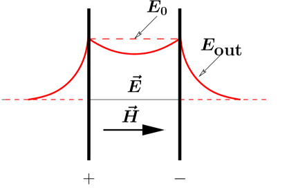
Figure -477: Capacitor in a magnetic field. The presence of extra dimensions or axion makes electric field massive. As a result electric field in the capacitor decreases; however, one can detect the presence of a non-zero electric field outside the plates of the capacitor.

To observe this effect, another type of experiment has been suggested in [31]. Namely, by placing a capacitor in a strong magnetic field, one can detect the redistribution of its electric field, in particular the appearance of an electric field outside the plates of a large capacitor (Fig. -477). In fact a similar effect would also be present in theories with ALP (this is discussed briefly in Appendix). We do not analyze here the feasibility of such an experiment, however, we want to notice that unlike the effects of rotation of polarization, the electric field $E_{\mathrm{out}}\sim m_{\gamma,H}$ depends linearly and not quadratically on the induced mass of the photon and therefore could in principle be stronger. Such an experiment would provide an independent test of the interpretation of PVLAS data. Moreover, this effect allows to differentiate between various types of models, determine separately mass and coupling constant of the axion, while its dependence on $H$ can differentiate between the 4-dimensional axion-like models and models with extra dimensions.

Acknowledgements

We would like to thank L. Alvarez-Gaumé, P. Sikivie, M. Shaposhnikov, and I. Tkachev for useful discussions. This work was supported in part by the European Commission under the RTN contract MRTN-CT-2004-503369 and in part by the INTAS contract 03-51-6346.

Appendix A Capacitor effect for one axion

A.1 Massless axion

Consider the Lagrangian of massless axion, interacting with the electromagnetic field

$$S_{\mathrm{axion}}=\mathop{\hskip-1.07639pt\int\hskip-1.72218pt}-\frac{1}{4}|F|^{2}+\frac{1}{2}|d\phi|^{2}+\frac{\phi}{4f_{\phi}}F_{\mu\nu}\tilde{F}^{\mu\nu}$$ (29)

In this case, equations of motion read

$$\partial_{\nu}F^{\mu\nu} =j_{0}^{\mu}+\frac{1}{2f_{\phi}}\epsilon^{\mu\nu\lambda\rho}\partial_{\nu}\phi F_{\lambda\rho}$$ (30)

$$\mathop{\Box}\phi =\frac{1}{f_{\phi}}\epsilon^{\mu\nu\lambda\rho}F_{\mu\nu}F_{\lambda\rho}$$ (31)

Their solution can be easily found in the case when the source term $j_{0}$ is just a (static) charge density $\rho(x)$ and the system is in the background constant magnetic field $H^{x}$. We choose static gauge, so that only $A_{0}$ is non-zero and solve Eq. (31) by writing

$$\partial_{x}\phi=\frac{H}{f_{\phi}}A_{0}$$ (32)

which reduces Eq. (30) to the Poisson equation

$$\partial_{x}^{2}A_{0}=\rho(x)+\frac{H^{2}}{f_{\phi}^{2}}A_{0}$$ (33)

with the mass of electric field being

$$m_{\gamma,H}^{2}=\frac{H^{2}}{f_{\phi}^{2}}.$$ (34)

We see that massless axion generates mass for static electric field (in the presence of a strong magnetic field) and thus in a capacitor experiment, similar to the one described in the section 4 (Fig. -477). The electric field outside the plates of the capacitor is given by $E_{out}\sim m_{\gamma,H}V_{0}$, where $V_{0}$ is the voltage applied to the plates of the capacitor. Unlike the effects of propagation of light in the magnetic field, the effect here (nonzero $E_{out}$) is proportional to the first power of magnetic mass $m_{\gamma,H}$.

A.2 Massive axion

Let us now consider modifications compared to the previous section (A.1) in the case when the axion has a mass $m_{\phi}$. Then, eqs.(30)–(31) become:

$$\partial_{\nu}F^{\mu\nu} =j_{0}^{\mu}+\frac{1}{2f_{\phi}}\epsilon^{\mu\nu\lambda\rho}\partial_{\nu}\phi F_{\lambda\rho}$$ (35)

$$\bigl{(}\mathop{\Box}+m_{\phi}^{2}\bigr{)}\phi =\frac{1}{4f_{\phi}}\epsilon^{\mu\nu\lambda\rho}F_{\mu\nu}F_{\lambda\rho}$$ (36)

Again, under the same assumptions (static charges $\rho(x)$, uniform background magnetic field) we get the following solution in Fourier space ($-i\partial_{x}\to k$)

$$\phi(x)=\frac{H}{f_{\phi}}\mathop{\hskip-1.07639pt\int\hskip-1.72218pt}\frac{dk}{2\pi}\frac{ike^{ikx}}{(k^{2}+m_{\phi}^{2})}A_{0}(k)$$ (37)

and for $A_{0}$:

$$A_{0}(x)=\mathop{\hskip-1.07639pt\int\hskip-1.72218pt}\frac{dk}{2\pi}\frac{e^{ikx}k^{2}}{(k^{2}+m_{\phi}^{2})(k^{2}+m_{\gamma,H}^{2})}\rho(k)$$ (38)

This integral is convergent and in the limit $m_{\phi}\to 0$ one recovers the solution of Eq. (33) of the massless axion. Let us analyze it for the simplest case $\rho(x)=q_{0}\delta(x)$ or $\rho(k)=q_{0}$:

$$A_{0}(x)=\frac{q_{0}}{4\pi}\left[e^{-m_{\phi}|x|}\frac{m_{\phi}}{m_{\phi}^{2}-m_{\gamma,H}^{2}}+e^{-m_{\gamma,H}|x|}\frac{m_{\phi}}{m_{\gamma,H}^{2}-m_{\phi}^{2}}\right]$$ (39)

In the interesting case $m_{\gamma,H}\ll m_{\phi}$ one finds

$$A_{0}(x)\approx A_{\mathrm{massless}}(x)\left\{\begin{aligned} \frac{m_{\gamma,H}^{2}}{m_{\phi}^{2}},&&|x|&\gg\frac{1}{m_{\phi}}\\ \frac{m_{\gamma,H}}{m_{\phi}},&&|x|&\ll\frac{1}{m_{\phi}}\end{aligned}\right.$$ (40)

i.e. the expression for the case of zero axion mass, suppressed by some power of $m_{\gamma,H}/m_{\phi}$.

References

- [1] E. Iacopini and E. Zavattini, Experimental method to detect the vacuum birefringence induced by a magnetic field, Phys. Lett. B85 (1979) 151.
- [2] P. Sikivie, Experimental tests of the *invisible* axion, Phys. Rev. Lett. 51 (1983) 1415.
- [3] A. A. Anselm, Axion photon oscillations in a steady magnetic field. (in russian), Yad. Fiz. 42 (1985) 1480–1483.
- [4] M. Gasperini, Axion production by electromagnetic fields, Phys. Rev. Lett. 59 (1987) 396–398.
- [5] L. Maiani, R. Petronzio, and E. Zavattini, Effects of nearly massless, spin zero particles on light propagation in a magnetic field, Phys. Lett. B175 (1986) 359.
- [6] G. Raffelt and L. Stodolsky, Mixing of the photon with low mass particles, Phys. Rev. D37 (1988) 1237.
- [7] PVLAS Collaboration, E. Zavattini et al., Experimental observation of optical rotation generated in vacuum by a magnetic field, Phys. Rev. Lett. 96 (2006) 110406, [hep-ex/0507107].
- [8] A. Ringwald, Axion interpretation of the pvlas data?, hep-ph/0511184.
- [9] G. G. Raffelt, Particle physics from stars, Ann. Rev. Nucl. Part. Sci. 49 (1999) 163–216, [hep-ph/9903472].
- [10] CAST Collaboration, K. Zioutas et al., First results from the cern axion solar telescope (cast), Phys. Rev. Lett. 94 (2005) 121301, [hep-ex/0411033].
- [11] E. Masso and J. Redondo, Evading astrophysical constraints on axion-like particles, JCAP 0509 (2005) 015, [hep-ph/0504202].
- [12] P. Jain and S. Mandal, Evading the astrophysical limits on light pseudoscalars, astro-ph/0512155.
- [13] E. Masso and J. Redondo, Compatibility of cast search with axion-like interpretation of pvlas results, hep-ph/0606163.
- [14] R. D. Peccei and H. R. Quinn, CP Conservation In The Presence Of Instantons, Phys. Rev. Lett. 38 (1977) 1440; Constraints Imposed By CP Conservation In The Presence Of Instantons, Phys. Rev. D 16 (1977) 1791.
- [15] S. Weinberg, A New Light Boson?, Phys. Rev. Lett. 40, 223 (1978); F. Wilczek, Problem Of Strong P And T Invariance In The Presence Of Instantons, Phys. Rev. Lett. 40 (1978) 279; J. E. Kim, Weak Interaction Singlet And Strong CP Invariance, Phys. Rev. Lett. 43 (1979) 103.
- [16] I. Antoniadis, A. Boyarsky, and O. Ruchayskiy, in preparation.
- [17] E. D’Hoker and E. Farhi, Decoupling a fermion whose mass is generated by a yukawa coupling: The general case, Nucl. Phys. B248 (1984) 59.
- [18] E. D’Hoker and E. Farhi, Decoupling a fermion in the standard electroweak theory, Nucl. Phys. B248 (1984) 77.
- [19] S. Eidelman et al., Review of Particle Physics, Phys. Lett. B 592 (2004) 1.
- [20] E. R. Williams, J. E. Faller, and H. A. Hill, New experimental test of coulomb’s law: A laboratory upper limit on the photon rest mass, Phys. Rev. Lett. 26 (1971) 721–724.
- [21] G. V. Chibisov, Astrophysical upper limits on the photon rest mass, Sov. Phys. Usp. 19 (1976) 624–626.
- [22] R. Lakes, Experimental limits on the photon mass and cosmic magnetic vector potential, Phys. Rev. Lett. 80 (1998) 1826–1829.
- [23] E. Adelberger, G. Dvali, and A. Gruzinov, Photon mass bound destroyed by vortices, hep-ph/0306245.
- [24] E. Fischbach and C. Talmadge, Ten years of the fifth force, hep-ph/9606249.
- [25] I. Antoniadis, E. Kiritsis, J. Rizos and T. N. Tomaras, D-branes and the standard model, Nucl. Phys. B 660 (2003) 81 [arXiv:hep-th/0210263]; P. Anastasopoulos, M. Bianchi, E. Dudas and E. Kiritsis, Anomalies, anomalous U(1)’s and generalized Chern-Simons terms, arXiv:hep-th/0605225.
- [26] L. D. Faddeev and S. L. Shatashvili, Algebraic and hamiltonian methods in the theory of nonabelian anomalies, Theor. Math. Phys. 60 (1985) 770–778.
- [27] C. Callan, and J. A. Harvey, Anomalies and fermion zero modes on strings and domain walls, Nucl. Phys. B250 (1985) 427.
- [28] X. G. Wen, Chiral luttinger liquid and the edge excitations in the fractional quantum hall states, Phys. Rev. B41 (1990) 12838–12844.
- [29] J. Frohlich and A. Zee, Large scale physics of the quantum hall fluid, Nucl. Phys. B364 (1991) 517–540.
- [30] A. Boyarsky, O. Ruchayskiy, and M. Shaposhnikov, Observational manifestations of anomaly inflow, Phys. Rev. D72 (2005) 085011, [hep-th/0507098].
- [31] A. Boyarsky, O. Ruchayskiy, and M. Shaposhnikov, Anomalies as a signature of extra dimensions, Phys. Lett. B626 (2005) 184–194, [hep-ph/0507195].