Parton transverse momenta
and direct photon production
in hadronic collisions
at high energies

Abstract

The invariant cross sections for direct photon production in hadron-hadron collisions are calculated for several initial energies (SPS, ISR, S$p\bar{p}$S, RHIC, Tevatron, LHC) including initial parton transverse momenta within the formalism of unintegrated parton distributions (UPDF). Different approaches from the literature are compared and discussed. A special emphasis is put on the Kimber-Martin-Ryskin (KMR) distributions and their extension into the soft region. Sum rules for UPDFs are formulated and discussed in detail. We find a violation of naive number sum rules for the KMR UPDFs. An interesting interplay of perturbative (large $k_{t}^{2}$) and nonperturbative (small $k_{t}^{2}$) regions of UPDFs in the production of both soft and hard photons is identified. The $k_{t}$-factorization approach with the KMR UPDFs is inconsistent with the collinear approach at large transverse momenta of photons. Kwieciński UPDFs provide very good description of all world data, especially at SPS and ISR energies. Off-shell effects are discussed and quantified. Predictions for the CERN LHC are given. Very forward/backward regions in rapidity at LHC energy are discussed and a possibility to test unintegrated gluon distributions (UGDF) is presented.

I Introduction

It was realized relatively early that the transverse momenta of initial (before a hard process) partons may play an important role in order to understand the distributions of produced direct photons, especially at small transverse momenta (see e.g.Owens ). The emitted photon may be produced directly in a hard process and/or from the fragmentation process. The latter process involves the parton-to-photon fragmentation functions which are not very well known. The isolation criterion used now routinly in the analysis of experimental data helps to reduce the second component almost completely.

The simplest way to include parton transverse momenta is via Gaussian smearing Owens ; WW98 ; AM04 . This phenomenological approach is not completely justified theoretically. One should remember that there are different reasons for nonzero transverse momenta of incoming partons. First is purely nonperturbative, related to the Fermi motion of true hadron constituents. The transverse momenta related to the internal motion of hadron constituents are believed to be not too large, definitely smaller than 1 GeV. The second is of dynamical nature, related to QCD effects involved in the evolution of the parton cascades. The latter effect may be strongly dependent on longitudinal momentum fraction of the parton taking part in the hard (sub)process.

The unintegrated parton distributions (UPDF) are the basic quantities that take into account explicitly the parton transverse momenta. The UPDFs have been studied recently in the context of different high-energy processes Gribov_Levin_Ryskin ; KMS97 ; HKSST1 ; HKSST2 ; Mariotto ; LS04 ; LS06 ; LZ05 ; LS05 . These works concentrated mainly on gluon degrees of fredom which play the dominant role in many processes at very high energies. At somewhat lower energies also quark and antiquark degrees of freedom become equally important. Recently the approach which dynamically includes transverse momenta of not only gluons but also of quarks and antiquarks was applied to direct-photon production LZ05 ; KMR_photons . In these calculations unintegrated parton distributions proposed by Kimber-Martin-Ryskin KMR were used. In this approach one assumes that the transverse momenta are generated only in the last step of the evolution ladder.

Up to now there is no complete agreement how to include evolution effects into the building blocks of the high-energy processes – the unintegrated parton distributions. In the present paper we shall discuss in detail a few approaches how to include transverse momenta of the incoming partons in order to calculate distributions of direct photons.

II Unintegrated parton distributions

In general, there are no simple relations between unintegrated and integrated parton distributions. Some of UPDFs in the literature are obtained based on familiar collinear distributions, some are obtained by solving evolution equations, some are just modelled or some are even parametrized. A brief review of unintegrated gluon distributions (UGDFs) that will be used also here can be found in Ref.LS06 . We shall not repeat all details concerning those UGDFs here. We shall discuss in more details only approaches which treat unintegrated quark/antiquark distributions.

In some of the approaches mentioned one imposes the following relation between the standard collinear distributions and UPDFs:

$$a(x,\mu^{2})=\int_{0}^{\mu^{2}}f_{a}(x,k_{t}^{2},\mu^{2})\frac{dk_{t}^{2}}{k_{t}^{2}}\;,$$ (1)

where $a=xq$ or $a=xg$.

Since familiar collinear distributions satisfy sum rules, one can define and test analogous sum rules for UPDFs. We shall discuss this issue in more detail in a separate section.

Below we shall discuss in detail some of the approaches for UPDFs. Some other approaches are discussed e.g. in Ref.LS06 .

II.1 Gaussian smearing

Due to its simplicity the Gaussian smearing of initial transverse momenta is a good reference point for other approaches. It allows to study phenomenologically the role of transverse momenta in several high-energy processes. We define simple unintegrated parton distributions:

$${\cal F}_{i}^{Gauss}(x,k_{t}^{2},\mu_{F}^{2})=xp_{i}^{coll}(x,\mu_{F}^{2})\cdot f_{Gauss}(k_{t}^{2})\;,$$ (2)

where $p_{i}^{coll}(x,\mu_{F}^{2})$ are standard collinear (integrated) parton distribution ($i=g,q,\bar{q}$) and $f_{Gauss}(k_{t}^{2})$ is a Gaussian two-dimensional function:

$$\begin{split}f_{Gauss}(k_{t}^{2})=\frac{1}{2\pi\sigma_{0}^{2}}\exp\left(-k_{t}^{2}/2\sigma_{0}^{2}\right)/\pi\;.\\ \;\end{split}$$ (3)

The UPDFs defined by Eq.(2) and (LABEL:Gaussian) are normalized such that:

$$\int{\cal F}_{i}^{Gauss}(x,k_{t}^{2},\mu_{F}^{2})\;dk_{t}^{2}=xp_{i}^{coll}(x,\mu_{F}^{2})\;.$$ (4)

II.2 KMR distributions

Kimber, Martin and Ryskin proposed a method to construct unintegrated parton distributions from the conventional DGLAP parton distributions KMR . Then

$$\begin{split}f_{a}(x,k_{t}^{2},\mu^{2})&=T_{a}(k_{t},\mu)\\ &\times\left[\frac{\alpha_{s}(k_{t}^{2})}{2\pi}\int_{x}^{1-\Delta}\sum_{a^{\prime}}P_{aa^{\prime}}(z)\;\;a^{\prime}\left(\frac{x}{z},k_{t}^{2}\right)dz\right]\;,\end{split}$$ (5)

where $P_{aa^{\prime}}(z)$ are splitting functions and $a^{\prime}\left(\frac{x}{z},k_{t}^{2}\right)$ are parton densities, where $a^{\prime}=\frac{x}{z}g$ or $\frac{x}{z}q$. Angular-ordering constraint $\Delta=\mu/(\mu+|k_{t}|)$ regulates the soft gluon singularities. Recently Lipatov and Zotov LZ05 used this method to calculate the direct photon spectra. Technically they did not use the original KMR method. Instead they have written

$$f_{q}(x,k_{t}^{2},\mu^{2})=T_{q}(k_{t}^{2},\mu^{2})\frac{\alpha_{s}(k_{t}^{2})}{2\pi}\int_{x}^{1}dz$$

$$\times \bigg{[}P_{qq}(z)\frac{x}{z}q\left(\frac{x}{z},k_{t}^{2}\right)\Theta(\Delta-z)+P_{qg}(z)\frac{x}{z}g\left(\frac{x}{z},k_{t}^{2}\right)\bigg{]}\;,$$

$$f_{g}(x,k_{t}^{2},\mu^{2})=T_{g}(k_{t}^{2},\mu^{2})\frac{\alpha_{s}(k_{t}^{2})}{2\pi}\int_{x}^{1}dz$$

$$\times \bigg{[}\sum_{q}P_{gq}(z)\frac{x}{z}q\left(\frac{x}{z},k_{t}^{2}\right)+P_{gg}(z)\frac{x}{z}g\left(\frac{x}{z},k_{t}^{2}\right)\Theta(\Delta-z)\bigg{]}\;.$$

In the following we shall call it LZ KMR prescription.

The virtual corrections are resummed via Sudakov form factors:

$${\mathrm{l}n}\;T_{q}(k_{t}^{2},\mu^{2})=-\int_{k_{t}^{2}}^{\mu^{2}}\frac{d{\mathrm{p}}_{t}^{2}}{{\mathrm{p}}_{t}^{2}}\frac{\alpha_{s}({\mathrm{p}}_{t}^{2})}{2\pi}\int_{0}^{z_{max}}dz\;P_{qq}(z)\;,$$ (8)

$${\mathrm{l}n}\;T_{g}(k_{t}^{2},\mu^{2})=-\int_{k_{t}^{2}}^{\mu^{2}}\frac{d{\mathrm{p}}_{t}^{2}}{{\mathrm{p}}_{t}^{2}}\frac{\alpha_{s}({\mathrm{p}}_{t}^{2})}{2\pi}\left[n_{f}\;\int_{0}^{1}dz\;P_{qg}(z)+\int_{z_{min}}^{z_{max}}dz\;z\;P_{gg}(z)\right]\;,$$ (9)

where $z_{max}=1-z_{min}=\mu/(\mu+|{\mathrm{p}}_{t}|)$.

The KMR method presented above can be used for transverse momenta $k_{t}^{2}>k_{t,0}^{2}$. In the present paper we assume saturation of UPDFs for $k_{t}^{2}<k_{t,0}^{2}$. This is a bit arbitrary procedure. We shall discuss the consequences of the procedure for physical observables.

II.3 Sum Rules for KMR UPDFs

In order to gain more insight into the KMR distributions described shortly in the previous section in the following section we shall formulate and check some sum rules.

Let us start from the valence number sum rules. We define the following integrals for up quarks:

$$\begin{split}N_{u_{val}}&(\mu^{2},k_{t,0}^{2})\equiv\int_{0}^{1}\frac{dx}{x}\int_{0}^{\mu^{2}}dk_{t}^{2}\\ &\times\left[f_{u}^{KMR}(x,k_{t}^{2},\mu^{2})-f_{\bar{u}}^{KMR}(x,k_{t}^{2},\mu^{2})\right]\\ \;\end{split}$$ (10)

and for down quarks:

$$\begin{split}N_{d_{val}}&(\mu^{2},k_{t,0}^{2})\equiv\int_{0}^{1}\frac{dx}{x}\int_{0}^{\mu^{2}}dk_{t}^{2}\\ &\times\left[f_{d}^{KMR}(x,k_{t}^{2},\mu^{2})-f_{\bar{d}}^{KMR}(x,k_{t}^{2},\mu^{2})\right]\;.\\ \;\end{split}$$ (11)

The parameter $k_{t,0}^{2}$ is implicit for the KMR distributions as discussed in the previous section. Naively one would expect: $N_{u_{val}}$ = 2 and $N_{d_{val}}$ = 1. We shall check the dependence of these quantities on $\mu^{2}$ and the freezing parameter $k_{t,0}^{2}$. The results are shown in Fig.1.

Figure 1: The number sum rule as a function of $\mu^{2}$ using standard KMR prescription with Sudakov form factor for up valence quarks (upper panel) and down valence quarks (lower panel) for several values of $k_{t,0}^{2}$.

Somewhat surprisingly the results depend strongly on $\mu^{2}$ and the freezing parameter $k_{t,0}^{2}$. The results are identical for the standard KMR prescription and the one proposed by Lipatov and Zotov. In the integrals above the parameter $\mu^{2}$ occurs as an argument of the parton distributions as well as the upper limit of the internal integral. It seems interesting to allow for independent parameters in the two places. Therefore we define new quantities for up quarks:

$$\begin{split}N^{0}_{u_{val}}&(\mu^{2},\mu_{0}^{2},k_{t,0}^{2})\equiv\int_{0}^{1}\frac{dx}{x}\int_{0}^{\mu^{2}}dk_{t}^{2}\\ &\times\left[f_{u}^{KMR}(x,k_{t}^{2},\mu_{0}^{2})-f_{\bar{u}}^{KMR}(x,k_{t}^{2},\mu_{0}^{2})\right]\\ \;\end{split}$$ (12)

and for down quarks:

$$\begin{split}N^{0}_{d_{val}}&(\mu^{2},\mu_{0}^{2},k_{t,0}^{2})\equiv\int_{0}^{1}\frac{dx}{x}\int_{0}^{\mu^{2}}dk_{t}^{2}\\ &\times\left[f_{d}^{KMR}(x,k_{t}^{2},\mu_{0}^{2})-f_{\bar{d}}^{KMR}(x,k_{t}^{2},\mu_{0}^{2})\right]\;.\\ \;\end{split}$$ (13)

The results for several $\mu_{0}^{2}$ are shown in Fig.2.

Figure 2: The modified number sum rule as a function of $\mu^{2}$ using standard KMR prescription with Sudakov form factor for up valence quarks (upper panel) and down valence quarks (lower panel) for several values of $\mu_{0}^{2}$.

Now a saturation of the sum rules for $\mu^{2}$ larger than 100 GeV² can be observed.

Another interesting quantity is:

$$xN^{0}_{i}(\mu^{2},\mu_{0}^{2},k_{t,0}^{2})\equiv\int_{0}^{1}dx\int_{0}^{\mu^{2}}\left[f_{i}^{KMR}(x,k_{t}^{2},\mu_{0}^{2})\right]\;dk_{t}^{2}$$ (14)

which can be interpreted as the contribution of parton of a given type $i$ to the momentum sum rule. In Fig.3 we show contributions for $g,u,\bar{u},d,\bar{d},s=\bar{s}$ as a function of the scale parameter $\mu^{2}$.

Figure 3: The momentum sum rule as a function of $\mu^{2}$ using standard KMR prescription (upper panel) and Lipatov-Zotov prescription (lower panel) with Sudakov form factor. Here $k_{t,0}^{2}=0.25$ GeV².

Again the defined above integrals are functions of the scale $\mu^{2}$. In this case there are huge differences for the standard (left panel) and LZ (right panel) prescription. These differences cancel as far as valence quarks are considered, which can be seen by inspection of Eq.(5) and/or Eq.(LABEL:LZ_KMR1), Eq.(LABEL:LZ_KMR2).

II.4 Kwieciński unintegrated parton distributions

Kwieciński has shown that the evolution equations for unintegrated parton distributions takes a particularly simple form in the variable conjugated to the parton transverse momentum. In the impact-parameter space the Kwieciński equation takes the following simple form

$${\partial{\tilde{f}_{NS}(x,b,\mu^{2})}\over\partial\mu^{2}}={\alpha_{s}(\mu^{2})\over 2\pi\mu^{2}}\int_{0}^{1}dz\,P_{qq}(z)$$

$$\times\bigg{[}\Theta(z-x)\,J_{0}((1-z)\mu b)\,{\tilde{f}_{NS}\left({x\over z},b,\mu^{2}\right)}-{\tilde{f}_{NS}(x,b,\mu^{2})}\bigg{]}\;,$$

$${\partial{\tilde{f}_{S}(x,b,\mu^{2})}\over\partial\mu^{2}}={\alpha_{s}(\mu^{2})\over 2\pi\mu^{2}}\int_{0}^{1}dz\bigg{\{}\Theta(z-x)\,J_{0}((1-z)\mu b)$$

$$\times\bigg{[}P_{qq}(z)\,{\tilde{f}_{S}\left({x\over z},b,\mu^{2}\right)}+P_{qg}(z)\,{\tilde{f}_{G}\left({x\over z},b,\mu^{2}\right)}\bigg{]}$$

$$-\bigg{[}zP_{qq}(z)+zP_{gq}(z)\bigg{]}\,{\tilde{f}_{S}(x,b,\mu^{2})}\bigg{\}}\;,$$

$${\partial{\tilde{f}_{G}(x,b,\mu^{2})}\over\partial\mu^{2}}={\alpha_{s}(\mu^{2})\over 2\pi\mu^{2}}\int_{0}^{1}dz\bigg{\{}\Theta(z-x)\,J_{0}((1-z)\mu b)$$

$$\times\bigg{[}P_{gq}(z)\,{\tilde{f}_{S}\left({x\over z},b,\mu^{2}\right)}+P_{gg}(z)\,{\tilde{f}_{G}\left({x\over z},b,\mu^{2}\right)}\bigg{]}$$

$$-\bigg{[}zP_{gg}(z)+zP_{qg}(z)\bigg{]}\,{\tilde{f}_{G}(x,b,\mu^{2})}\bigg{\}}\;.$$

(15)

We have introduced here the short-hand notation

$$\begin{split}\tilde{f}_{NS}&=\tilde{f}_{u}-\tilde{f}_{\bar{u}},\;\;\tilde{f}_{d}-\tilde{f}_{\bar{d}}\;,\\ \tilde{f}_{S}&=\tilde{f}_{u}+\tilde{f}_{\bar{u}}+\tilde{f}_{d}+\tilde{f}_{\bar{d}}+\tilde{f}_{s}+\tilde{f}_{\bar{s}}\;.\end{split}$$ (16)

The unintegrated parton distributions in the impact factor representation are related to the familiar collinear distributions as follows

$$\tilde{f}_{k}(x,b=0,\mu^{2})=\frac{x}{2}p_{k}(x,\mu^{2})\;.$$ (17)

On the other hand, the transverse momentum dependent UPDFs are related to the integrated parton distributions as

$$xp_{k}(x,\mu^{2})=\int_{0}^{\infty}dk_{t}^{2}\;f_{k}(x,k_{t}^{2},\mu^{2})\;.$$ (18)

The two possible representations, in the momentum space and in the impact parameter space, are interrelated via Fourier-Bessel transform

$$\begin{split}&{f_{k}(x,k_{t}^{2},\mu^{2})}=\int_{0}^{\infty}db\;bJ_{0}(k_{t}b){{\tilde{f}}_{k}(x,b,\mu^{2})}\;,\\ &{{\tilde{f}}_{k}(x,b,\mu^{2})}=\int_{0}^{\infty}dk_{t}\;k_{t}J_{0}(k_{t}b){f_{k}(x,k_{t}^{2},\mu^{2})}\;.\end{split}$$ (19)

The index k above numerates either gluons (k=0), quarks (k$>$ 0) or antiquarks (k$<$ 0). While physically $f_{k}(x,k_{t}^{2},\mu^{2})$ should be positive, there is no obvious reason for such a limitation for $\tilde{f}_{k}(x,b,\mu^{2})$.

In the following we use leading-order parton distributions from Ref.GRV98 as the initial condition for QCD evolution. The set of integro-differential equations in b-space was solved by the method based on the discretisation made with the help of the Chebyshev polynomials (see Kwiecinski ). Then the unintegrated parton distributions were put on a grid in $x$, $b$ and $\mu^{2}$ and the grid was used in practical applications for Chebyshev interpolation.

For the calculation of inclusive and coincidence cross section for the photon production (see next section) the parton distributions in momentum space are more useful. These calculation requires a time-consuming multi-dimensional integrations. Therefore an explicit calculation of the momentum-space of the Kwieciński UPDFs via Fourier transform for needed in the main calculation values of $(x_{1},k_{1,t}^{2})$ and $(x_{2},k_{2,t}^{2})$ (see next section) is not possible. Therefore it becomes a neccessity to prepare auxiliary grids of the momentum-representation UPDFs before the actual calculation of the cross sections. These grids are then used via a two-dimensional interpolation in the spaces $(x_{1},k_{1,t}^{2})$ and $(x_{2},k_{2,t}^{2})$ associated with each of the two incoming partons.

The evolution of the parton cascade leads to a spread of the transverse momentum of the parton at the end of the cascade (the parton participating in a hard process). Let us define the following measure of the spread:

$$<k_{t}^{2}>_{f_{k}}(x,\mu^{2})\equiv\frac{\int dk_{t}^{2}\;k_{t}^{2}\;f_{k}(x,k_{t}^{2},\mu^{2})}{\int dk_{t}^{2}\;f_{k}(x,k_{t}^{2},\mu^{2})}\;.$$ (20)

Above $f_{k}$ can be either gluon ($k=0$) or quark ($k>0$) or antiquark ($k<0$) distribution. As an example in Fig.4 we show the spread, obtained for different parton species, as a function of parton longitudinal momentum fraction.

Figure 4: $<k_{t}^{2}>$ as a function of $x$ for different unintegrated parton distributions: solid - glue, dashed - $u_{val}$, dotted - $d_{val}$ and dash-dotted - sea.

In this calculation the factorization scale was fixed at $\mu^{2}=$ 100 GeV². The Kwieciński evolution leads to increasing spread with decreasing longitudinal momentum fraction. The spread for different species of partons is quite different. In the region of small $x$ the spread in $k_{t}^{2}$ for gluons is bigger than a similar spread for sea and valence quarks. This is very different than a corresponding spread for Gaussian distributions which is usually taken to be independent of $x$ and parton species. In addition, the spread of $k_{t}^{2}$ for small values of $x$ is considerably larger than the nonperturbative spread of the initial Gaussian distributions, taken here identical for all species and encoded in the model parameter $b_{0}$.

In contrast to the KMR unintegrated valence quark distributions the Kwieciński valence quark distributions fulfill the number sum rules for up:

$$\begin{split}N_{u_{val}}(\mu^{2})&=\int_{0}^{1}\frac{dx}{x}\int_{0}^{\infty}\;dk_{t}^{2}\\ &\times\left[f_{u}^{Kwiec}(x,k_{t}^{2},\mu^{2})-f_{\bar{u}}^{Kwiec}(x,k_{t}^{2},\mu^{2})\right]=2\\ \;\end{split}$$ (21)

and for down quarks:

$$\begin{split}N_{d_{val}}(\mu^{2})&=\int_{0}^{1}\frac{dx}{x}\int_{0}^{\infty}\;dk_{t}^{2}\\ &\times\left[f_{d}^{Kwiec}(x,k_{t}^{2},\mu^{2})-f_{\bar{d}}^{Kwiec}(x,k_{t}^{2},\mu^{2})\right]=1\;.\end{split}$$ (22)

II.5 Mixed distributions

The calculation with the Kwieciński distributions discussed in the previous section shows that the spread in $k_{t}^{2}$ for gluons can be much bigger than that for quarks/antiquarks. On the other hand in the region of small $x$ there are several unintegrated gluon distributions available in the literature. At high energy (small $x$) the contribution of $qg$, $gq$ subprocesses is larger than the contribution of $q\bar{q}$, $\bar{q}q$ subprocesses. Therefore it seems reasonable to use the different UGDFs from the literature together with the Gaussian distributions for quarks and antiquarks as discribed above. Such an approach is especially justified at forward ($y_{\gamma}\gg$ 0) and backward photon rapidities ($y_{\gamma}\ll$ 0), where $x_{1}\ll$ 1, $x_{2}\sim$ 1 ($\langle k_{1,t}\rangle_{glue}>\langle k_{2,t}\rangle_{q,\bar{q}}$) or $x_{1}\sim$ 1, $x_{2}\ll$ 1 ($\langle k_{1,t}\rangle_{q\bar{q}}<\langle k_{2,t}\rangle_{glue}$).

III UPDFs and photon production

The cross section for the production of a photon and an associated parton (jet) can be written as

$$\frac{d\sigma(h_{1}h_{2}\rightarrow\gamma,parton)}{d^{2}p_{1,t}d^{2}p_{2,t}} = \int dy_{1}dy_{2}\frac{d^{2}k_{1,t}}{\pi}\frac{d^{2}k_{2,t}}{\pi}\frac{1}{16\pi^{2}(x_{1}x_{2}s)^{2}}\;\sum_{i,j,k}\overline{|\mathcal{M}(ij\rightarrow\gamma k)|^{2}}$$ (23)

$$\cdot \delta^{2}(\vec{k}_{1,t}+\vec{k}_{2,t}-\vec{p}_{1,t}-\vec{p}_{2,t})f_{i}(x_{1},k_{1,t}^{2})f_{j}(x_{2},k_{2,t}^{2})\;,$$

where $\vec{k}_{1,t}$ and $\vec{k}_{2,t}$ are transverse momenta of incoming partons. The longitudinal momentum fractions are calculated as

$$x_{1}=\frac{m_{1t}}{\sqrt{s}}\mathrm{e}^{-y_{1}}+\frac{m_{2t}}{\sqrt{s}}\mathrm{e}^{-y_{2}}\;,$$ (24)

$$x_{2}=\frac{m_{1t}}{\sqrt{s}}\mathrm{e}^{y_{1}}+\frac{m_{2t}}{\sqrt{s}}\mathrm{e}^{y_{2}}\;,$$ (25)

where $m_{1t}$ and $m_{2t}$ are respective transverse masses. In the leading-order approximation: $(i,j,k)=(q,{\bar{q}},g),({\bar{q}},q,g),(q,g,q),(g,q,q)$, etc. (see Fig.5).

Figure 5: The diagrams included in our $k_{t}$-factorization approach with the notation of kinematical variables.

If one makes the following replacements

$$f_{i}(x_{1},k_{1,t}^{2})\rightarrow x_{1}p_{i}(x_{1})\delta(k_{1,t}^{2})$$ (26)

and

$$f_{j}(x_{2},k_{2,t}^{2})\rightarrow x_{2}p_{j}(x_{2})\delta(k_{2,t}^{2})$$ (27)

then one recovers the standard collinear formula (see e.g.Owens ).

The inclusive invariant cross section for direct photon production can be written

$$\begin{split}\frac{d\sigma(h_{1}h_{2}\to\gamma)}{dy_{1}d^{2}p_{1,t}}&=\int dy_{2}\frac{d^{2}k_{1,t}}{\pi}\frac{d^{2}k_{2,t}}{\pi}\left(...\right)|_{\vec{p}_{2,t}=\vec{k}_{1,t}+\vec{k}_{2,t}-\vec{p}_{1,t}}\\ &=\int dk_{1,t}dk_{2,t}\;I(k_{1,t},k_{2,t};y_{1},p_{1,t})\;.\end{split}$$ (28)

and analogously the cross section for the associated parton (jet) can be written

$$\frac{d\sigma(h_{1}h_{2}\to k)}{dy_{2}d^{2}p_{2,t}}=\int dy_{1}\frac{d^{2}k_{1,t}}{\pi}\frac{d^{2}k_{2,t}}{\pi}\left(...\right)|_{\vec{p}_{1,t}=\vec{k}_{1,t}+\vec{k}_{2,t}-\vec{p}_{2,t}}\;.$$ (29)

The integrand $I(k_{1,t},k_{2,t};y_{1},p_{1,t})$ defined in Eq.(28) depends strongly on UPDFs used. We shall return to this interesting issue.

Let us return to the coincidence cross section. The integration with the Dirac delta function in (23)

$$\int dy_{1}dy_{2}\frac{d^{2}k_{1,t}}{\pi}\frac{d^{2}k_{2,t}}{\pi}\left(...\right)\delta^{2}(...)$$ (30)

can be performed by introducing the following new auxiliary variables:

$$\vec{Q}_{t} = \vec{k}_{1,t}+\vec{k}_{2,t}\;,$$

$$\vec{q}_{t} = \vec{k}_{1,t}-\vec{k}_{2,t}\;.$$ (31)

The jacobian of this transformation is:

$$\frac{\partial(\vec{Q}_{t},\vec{q}_{t})}{\partial(\vec{k}_{1,t},\vec{k}_{2,t})}=\begin{pmatrix}1&1\\ 1&-1\\ \end{pmatrix}\cdot\begin{pmatrix}1&1\\ 1&-1\\ \end{pmatrix}=2\cdot 2=4\;.$$ (32)

Then our initial cross section can be written as:

$$\begin{split}\frac{d\sigma(h_{1}h_{2}\rightarrow\gamma,parton)}{d^{2}p_{1,t}d^{2}p_{2,t}}&=\frac{1}{4}\int dy_{1}dy_{2}\;d^{2}Q_{t}d^{2}q_{t}\;\;\;(...)\;\delta^{2}(\vec{Q}_{t}-\vec{p}_{1,t}-\vec{p}_{2,t})\\ &=\frac{1}{4}\int dy_{1}dy_{2}\;\;\;\;\;\;\;\underbrace{d^{2}q_{t}}\;\;\;\;\;\left(...\right)\;|_{\vec{Q}_{t}=\vec{P}_{t}}\\ &=\frac{1}{4}\int dy_{1}dy_{2}\;\;\;\;\overbrace{\underbrace{q_{t}dq_{t}}\;d\varphi}\;\left(...\right)\;|_{\vec{Q}_{t}=\vec{P}_{t}}\\ &=\frac{1}{4}\int dy_{1}dy_{2}\;\overbrace{\frac{1}{2}dq_{t}^{2}\;d\varphi}\;\;\;\;\left(...\right)\;|_{\vec{Q}_{t}=\vec{P}_{t}}\;.\end{split}$$ (33)

Above $\vec{P}_{t}=\vec{p}_{1,t}+\vec{p}_{2,t}$. Different representations of the cross section are possible. If one is interested in the distribution of the sum of transverse momenta of the outgoing particles (parton and photon), then it is convenient to write

$$d^{2}p_{1,t}\;d^{2}p_{2,t} = \frac{1}{4}d^{2}P_{t}d^{2}p_{t}=\frac{1}{4}d\varphi_{+}P_{t}dP_{t}\;d\varphi_{-}p_{t}dp_{t}$$ (34)

$$= \frac{1}{4}\;2\pi P_{t}dP_{t}\;d\varphi_{-}p_{t}dp_{t}\;.$$

If one is interested in studying a two-dimensional map $p_{1,t}\times p_{2,t}$ then the differential volume element can be written

$$d^{2}p_{1,t}\;d^{2}p_{2,t}=d\phi_{1}\;p_{1,t}dp_{1,t}\;d\phi_{2}\;p_{2,t}dp_{2,t}\;.$$ (35)

Then the two-dimensional map can be written as

$$\frac{d\sigma(p_{1,t},p_{2,t})}{dp_{1,t}dp_{2,t}}=\int d\phi_{1}d\phi_{2}p_{1,t}p_{2,t}\int dy_{1}dy_{2}\frac{1}{4}q_{t}dq_{t}d\phi_{q_{t}}\left(...\right).$$ (36)

The integrals over $\phi_{1}$ and $\phi_{2}$ must be the most external ones. The integral above is formally a 6-dimensional one. It is convenient to make the following transformation of variables

$$(\phi_{1},\phi_{2})\to\left(\phi_{sum}=\phi_{1}+\phi_{2},\;\phi_{dif}=\phi_{1}-\phi_{2}\right)\;,$$ (37)

Explicit formulae for the basic matrix elements are given in Appendix B.

IV Inclusive photon spectra

IV.1 Integrands of the inclusive cross sections

Before we go to the discussion of the dependence of the invariant cross sections on the values of rapidity and photon transverse momentum let us consider the integrand $I(k_{1,t},k_{2,t};y_{1},p_{1,t})$ (before integration over $k_{1,t}$ and $k_{2,t}$) in Eq.(28).

In Fig.6 we show an example for $\sqrt{s}$ = 63 GeV, $y$ = 0 and $p_{t,\gamma}$ = 5 GeV. In this calculation the unintegrated parton distributions based on GRV collinear parton distributions GRV95 and Gaussian smearing ($\sigma_{0}$ = 1 GeV) in parton transverse momenta were used. This is a rather standard method to “improve” the collinear approach. We do not need to mention that this, although having some physical motivation, is a rather ad hoc procedure. The two-dimensional distributions are peaked for small values of $k_{1,t}$ and $k_{2,t}$. How fast the distribution decreases with $k_{1,t}$ and/or $k_{2,t}$ depends on the value of the smearing parameter $\sigma_{0}$. The larger $\sigma_{0}$ the slower the decrease.

Figure 6: Integrand under the $k_{1,t}$ and $k_{2,t}$ integration in the invariant cross section formula for proton-proton scattering at $\sqrt{s}=63$ GeV and y= 0, $p_{t,\gamma}$ = 5 GeV and Gaussian UPDFs ($\sigma_{0}$ = 1 GeV). Off-shell matrix elements for gluons are used. (a) $q\bar{q}$, (b) $\bar{q}q$, (c) $gq$, (d) $qg$.

In Fig.7 we show similar maps ($\sqrt{s}$ = 63 GeV, $y$ = 0, $p_{t,\gamma}$ = 5 GeV) for the KMR UPDFs.

Figure 7: Integrand under the $k_{1,t}$ and $k_{2,t}$ integration in the invariant cross section formula for proton-proton scattering at $\sqrt{s}=63$ GeV and y= 0, $p_{t,\gamma}$ = 5 GeV and KMR UPDFs ($k_{t,0}^{2}$ = 0.25 GeV²). Off-shell matrix elements for gluons are used. (a) $q\bar{q}$, (b) $\bar{q}q$, (c) $gq$, (d) $qg$.

Three local maxima can be seen in the figure. A first maximum occurs when both $k_{1,t}$ and $k_{2,t}$ are very small. This is caused by the structure of UPDFs themselves. The two other maxima occur when $k_{1,t}=p_{t}$ and $k_{2,t}$ is small or $k_{2,t}=p_{t}$ and $k_{1,t}$ is small. These are caused by the structure of matrix elements. The presence of long tails in $k_{t}$ in the KMR distributions is a necessary condition to produce the second and third maxima. When $p_{t}$ increases the second and third maxima move towards larger $k_{1,t}$ and/or $k_{2,t}$. This clearly shows that the range of integration must depend on the value of photon transverse momentum. In Fig.8 we show some integrand (KMR UPDFs) but for larger energy $W=630$ GeV and larger photon transverse momentum $p_{t,\gamma}=50$ GeV.

Figure 8: Integrand under the $k_{1,t}$ and $k_{2,t}$ integration in the invariant cross section formula for proton-antiproton scattering at $\sqrt{s}=630$ GeV and y= 0, $p_{t,\gamma}$ = 50 GeV and KMR UPDFs ($k_{t,0}^{2}$ = 0.25 GeV²). Off-shell matrix elements for gluons are used. (a) $q\bar{q}$, (b) $\bar{q}q$, (c) $gq$, (d) $qg$.

Fig.8 looks very much the same as Fig.7 if the transverse momenta of incoming partons are rescaled by the ratio of photon transverse momenta.

In Fig.9 we show a similar map for the Kwieciński distributions. In this case the factorization scale is fixed for $\mu^{2}$ = 100 GeV².

Figure 9: Integrand under $k_{1,t}$ and $k_{2,t}$ in the invariant cross section formula for proton-proton scattering at $\sqrt{s}=63$ GeV and y= 0, $p_{t,\gamma}$ = 5 GeV and Kwieciński UGDF ($b_{0}$ = 1 GeV^-1, $\mu^{2}$ = 100 GeV²). Off-shell matrix elements for gluons are used. (a) $q\bar{q}$, (b) $\bar{q}q$, (c) $gq$, (d) $qg$.

All kinematical variables are exactly the same as in the previous cases. The integrand is rather similar to the one for the KMR UPDFs, except that the first maximum at $k_{1,t},k_{2,t}\approx$ 0 is somewhat broader. We shall see consequences of the different integrands when discussing transverse momentum dependence of the photon inclusive cross sections.

IV.2 Off-shell effects

Let us quantify the kinematical off-shell effect by defining the following quantities:

$$\begin{split}&R_{qg}(k_{1,t}^{2},k_{2,t}^{2})&=&\frac{I_{qg}^{off-shell}(k_{1,t}^{2},k_{2,t}^{2})}{I_{qg}^{on-shell}(k_{1,t}^{2},k_{2,t}^{2})}\;,\\ &R_{gq}(k_{1,t}^{2},k_{2,t}^{2})&=&\frac{I_{gq}^{off-shell}(k_{1,t}^{2},k_{2,t}^{2})}{I_{gq}^{on-shell}(k_{1,t}^{2},k_{2,t}^{2})}\;.\end{split}$$ (38)

In Fig.10 we present results for $R_{gq}$ (left panels) and $R_{qg}$ (right panels) for proton-proton scattering at W = 63 GeV ($y_{\gamma}$ = 0, $p_{\gamma,t}$ = 5 GeV) and proton-antiproton scattering at W = 630 GeV ($y_{\gamma}$ = 0, $p_{\gamma,t}$ = 50 GeV).

Figure 10: Off-shell effects for the dominant mechanisms for $pp$ scattering at $\sqrt{s}$ = 63 GeV, y = 0, $p_{t}$ = 5 GeV (upper panels) and $p\bar{p}$ scattering at $\sqrt{s}$ = 630 GeV, y = 0, $p_{t}$ = 50 GeV (lower panels).

When $k_{1,t},k_{2,t}\to$ 0 the off-shell effects dissapear, i.e. the ratio becomes unity. The larger transverse momenta of gluons the larger the off-shell effect is. Therefore one may expect a related enhancement of the photon inclusive cross section when the UGDFs with large transverse momentum spread are used.

In Fig.11 we show the ratio of the inclusive cross sections obtained with off-shell and on-shell matrix elements as a function of photon transverse momentum.

Figure 11: The ratio of inclusive cross sections with off-shell and on-shell matrix elements with Gaussian UPDFs and different values of the parameter $\sigma_{0}$ as a function of photon transverse momentum.

In this calculation the Gaussian distributions were used with different values of the $\sigma_{0}$ parameter. The bigger $\sigma_{0}$ the larger the enhancement due to the off-shell effects.

In Fig.12 we show similar enhancement for a few representative UPDFs discussed in section 2.

Figure 12: The ratio of inclusive cross sections with off-shell and on-shell matrix elements for different UPDFs as a function of photon transverse momentum.

The biggest enhancement is obtained with the KMR and BFKL distributions, i.e. those which have the biggest gluon transverse momentum spread. In general, the bigger photon transverse momentum, the smaller the enhancement. We conclude that at larger photon transverse momenta one can use standard on-shell matrix elements.

IV.3 Photon transverse momentum distributions

Let us start the analysis from the lowest energies. In Fig.13 we show inclusive invariant cross section as a function of Feynman $x_{F}$ for several experimental values of photon transverse momenta as measured by the WA70 collaboration.

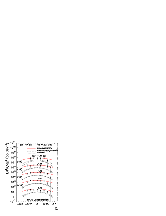
Figure 13: Invariant cross section for direct photons for $\sqrt{s}$ = 23 GeV as a function of Feynman $x_{F}$ for different bins of transverse momenta. In this calculation of shell matrix elements for subprocesses with gluons were used. The Kwieciński UPDFs were calculated with the factorization scale $\mu^{2}$ = 100 GeV². The theoretical results are compared with the WA70 collaboration data data_WA70 .

It is well known that the collinear approach (dotted line) fails to describe the low transverse momentum data by a sizeable factor of 4 or even more. Also the $k_{t}$-factorization result with the KMR UPDFs (dashed line) underestimate the low-energy data. In contrast, the Kwieciński UPDFs (solid line) describe the WA70 collaboration data almost perfect. In order to illustrate the situation in Fig.14 we show the ratio

$$\frac{d\sigma^{Kwiec}}{dyd^{2}p_{t}}(x_{F},p_{t})\bigg{/}\frac{d\sigma^{coll}}{dyd^{2}p_{t}}(x_{F},p_{t})$$ (39)

as a function of Feynman $x_{F}$ for $p_{t}$ = 4.11 GeV and $p_{t}$ = 5.70 GeV.

Figure 14: The ratio of the invariant cross sections as a function of $x_{F}$ for $\sqrt{s}$ = 23 GeV. The Kwieciński UPDFs were calculated with the factorization scale $\mu^{2}$ = 100 GeV².

This figure shows that the enhancement factor strongly depends on $x_{F}$. Such an enhancement is required by the experimental data as can be seen by inspection of the previous figure.

In Fig.15 we show invariant cross section for direct photon production as a function of photon transverse momentum for photon rapidity $y$ = 0 and $\sqrt{s}$ = 63 GeV.

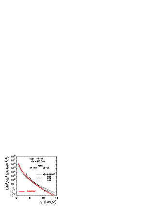
Figure 15: Invariant cross section for direct photons for $\sqrt{s}$ = 63 GeV and $y$ = 0 as a function of photon transverse momentum. In this calculation off-shell matrix element for gluons were used. The experimental data of the R806 collaboration are taken from Ref.data_R806 . (a) Gaussian smearing ($\sigma_{0}$ = 1, 2 GeV) versus collinear approach (b) standard KMR prescription,

The results obtained with the KMR UPDFs strongly depend on the value of the parameter $k_{t,0}^{2}$. The larger the parameter $k_{t,0}^{2}$, the smaller cross section. This means that even at large photon transverse momenta the nonperturbative effects (small $k_{t}$’s) play an important role. This can be better understood via inspection of the two-dimensional maps $k_{1,t}\times k_{2,t}$ shown in Fig.7 and is related to the second and third local maxima which give a significant contribution to the invariant cross section.

In principle, one could try to find the parameter $k_{t,0}^{2}$ by confronting the theoretical results with experimental data. If the parameter is adjusted to larger transverse momenta there is a deficit at smaller transverse momenta compared to the ISR data data_R806 .

In Fig.16 we compare our results with recent proton-proton RHIC data data_PHENIX .

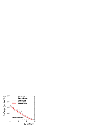
Figure 16: Invariant cross section for direct photons for $\sqrt{s}=200$ GeV and $y$ = 0. In this calculation off-shell matrix element for gluons were used. The experimental data of the PHENIX collaboration are taken from Ref.data_PHENIX . (a) standard KMR prescription (b) Gaussian smearing ($\sigma_{0}$ = 1, 2 GeV) versus Kwieciński and collinear approach

Here only low transverse-momenta of photons were measured. The results obtained with the Gaussian UPDFs strongly depend on the value of the $\sigma_{0}$ parameter which is not surprising for the low transverse momenta. The Kwieciński distributions give fairly good description of the PHENIX data.

In contrast to the “low energy” data, there is no deficit for the KMR UPDFs at larger energies as can be seen from Figs. 17, 18 and 19.

Figure 17: Invariant cross section for direct photons for $\sqrt{s}=630$ GeV. In this calculation off-shell matrix element for gluons were used. The experimental data of the UA2 collaboration were taken from Ref.data_UA2 . (a) Gaussian smearing, (b) quark/antiquarks: Gaussian smearing ($\sigma_{0}$ = 1 GeV), gluons: KL, BFKL and GBW, (c) standard KMR prescription.

Figure 18: Invariant cross section for direct photons for $\sqrt{s}=1800$ GeV. In this calculation off-shell matrix element for gluons was used. (a) standard KMR prescription, (b) quarks/antiquarks: Gaussian smearing ($\sigma_{0}$ = 1 GeV), gluons: KL, BFKL and GBW.

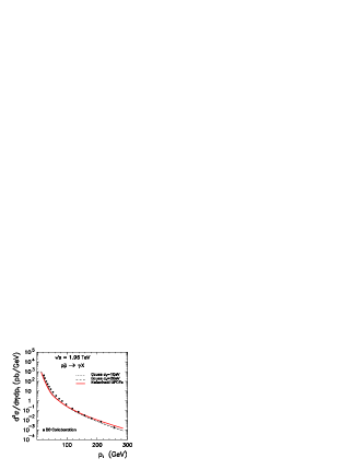
Figure 19: Cross section for direct photons for $\sqrt{s}=1.96$ TeV. In this calculation off-shell matrix element for gluons were used. (a) standard KMR prescription, (b) Gaussian smearing ($\sigma_{0}$ = 1,2 GeV) versus Kwieciński UPDFs.

The KMR UPDFs, however, strongly overestimate the experimental data at large photon transverse momenta. This is especially visible for proton-antiproton collisions at W = 1.96 TeV when compared with recent Tevatron (run 2) data data_D0_w1960 . Figs.18 and 19 show that the unintegrated parton distribution approach with the KMR UPDFs is clearly inconsistent with the standard collinear approach at large transverse momenta. This is caused by the presence of large-$k_{t}$ tails (of the 1/$k_{t}$ type) in the KMR UPDFs. It is not the case for the Gaussian and Kwieciński UPDFs which seem to converge to the standard collinear result at large photon transverse momenta. In this respect the latter UPDFs seems preferable.

IV.4 Direct photons at LHC

Up to now we have confronted our results with the existing experimental data from SPS, ISR, RHIC, S$p\bar{p}$S and Tevatron. In a not too distant future one may expect experimental data from a newly constructed LHC.

In Fig.20 we present transverse momentum dependence of the invariant cross section for the proton-proton collisions at W = 14 TeV for different values of photon rapidities.

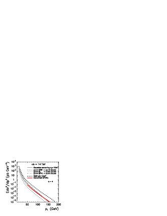
Figure 20: Predictions for LHC ($\sqrt{s}$ = 14 TeV) for different photon rapidities y = 0, 2, 4. We compare results for different UPDFs: KMR($k_{t,0}^{2}$ = 1 GeV²), GRV+Gaussian smearing ($\sigma_{0}$ = 1 GeV) and BFKL, KL and GBW UGDFs with quarks/antiquarks smeared by a Gaussian distribution ($\sigma_{0}$ = 1 GeV).

Different UPDFs lead to quite different results at the LHC energies. Therefore future measurements at LHC should give a chance to verify different UPDFs discussed here as well as others to be constructed in the future.

In Fig.21 we display average values of $x_{1}$ and $x_{2}$ of partons participating in a hard subprocess for two values of the photon transverse momentum $p_{t}$ = 10, 50 GeV.

Figure 21: Average values of $x_{1}$ (solid) and $x_{2}$ (dashed) as a function of photon rapidity. The borders of the bands shown correspond to $p_{t}$ = 10 GeV (lower limit) ant $p_{t}$ = 50 GeV (upper limit).

Figure 22: The dominant mechansisms of photon production at forward (left panel) and backward (right panel) rapidities.

At large rapidities either $x_{1}\gg x_{2}$ or $x_{1}\ll x_{2}$. Then one expects the dominance of $q(valence)g$ or $gq(valence)$ hard processes (see Fig.22). At such small values of $x$ the evolution effects for UGDFs are expected to be very important. In addition, one expects rather small transverse momenta of large-x valence quarks, much smaller than transverse momenta of the associated small-x gluons.

In Fig.23 we show the dependence of the invariant cross section on photon rapidity for fixed values of the photon transverse momenta.

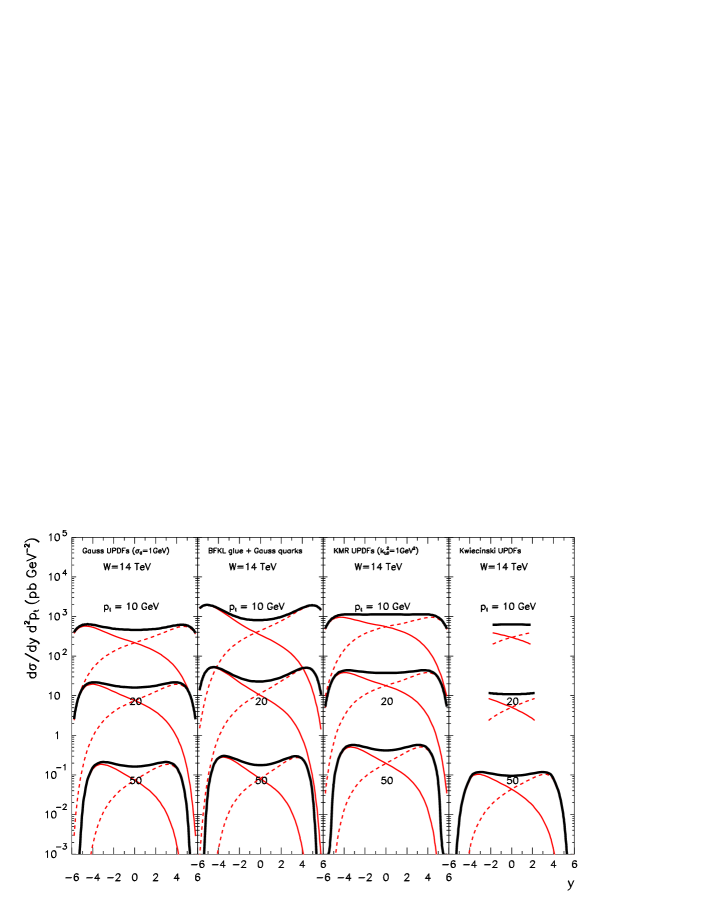
Figure 23: The rapidity dependence of the invariant cross section for a few values of photon transverse momenta ($p_{t}$ = 10, 20, 50 GeV). The contribution of $gq$ (solid) and $qg$ (dashed) subprocesses are shown separately for each value of the transverse momentum.

Results obtained with different UGDFs differ significantly in the region of large rapidities.

In the case of the Kwieciński UPDFs at small transverse momenta ($p_{t}=10,20$ GeV) only limited part of the full curve is shown. This is dictated by a purely technical cut on the longitudinal momentum fraction $x>10^{-4}$ when constructing interpolation maps of the Kwieciński UPDFs. As can be seen from Fig.21 large $|y|$ require very small $x_{1}$ or $x_{2}$, sometimes smaller than $10^{-4}$. Furthermore the Kwieciński distributions are not expected to be reliable at such small values of longitudinal momentum fractions. Therefore the range of application of the Kwieciński UPDFs at LHC is limited in rapidity and photon transverse momentum. The larger photon transverse momentum, the broder range of application in photon rapidity.

In conclusion, the region of large rapidities ($|y|>$ 3), discussed in this section, seems an appropriate place to test models of UPDFs. It is not clear to us if any of the LHC detectors can register the large-energy forward/backward photons. The CASTOR detector associated with the CMS detector is a potential option.

V Conclusions

The inclusive cross section for prompt photon production has been calculated for different incident energies from SPS to LHC within the formalism of unintegrated parton distributions. Different models of UPDFs lead to rather different results. The Kwieciński distributions provide the best description of experimental data in the broad range of incident energies. The existing experimental data test UPDFs down to x = 10^-3, i.e. in the region of intermediate longitudinal momentum fractions adequate for application of the Kwieciński equations. Inclusion of the QCD evolution effects and especially their effect on initial parton transverse momenta allowed to solve the long-standing problem of theoretical understanding the low energy and low transverse momentum data for direct photon production.

As a buy-product we have analyzed momentum sum rule for different UPDFs. We have found that the KMR UPDFs violate naive number sum rules. The same distributions lead to an interesting interplay of soft (small gluon $k_{t}$’s) and hard (large gluon $k_{t}$’s) regions of UPDFs. Even at large photon transverse momenta this interplay causes a huge enhancement as compared to collinear approach, quite inconsistent with the experimental data at large photon transverse momenta.

We have presented predictions for LHC based on several UPDFs with special emphasis on large rapidity region. Here different UPDFs lead to quite different predictions. Therefore we conclude that this region can be very useful to test different UPDFs.

VI Acknowledgments

We are indebted to Artem Lipatov for an interesting and instructive discusion concerning their work on direct photon production. This paper was partially supported by the grant of the Polish Ministry of Scientific Research and Information Technology number 1 P03B 028 28.

VII Appendix A

The moving with center-of-mass hadron-hadron energy maxima for the KMR distributions cause that the integration in $dk_{1,t}$ and $dk_{2,t}$ is not very efficient, especially for large $p_{t}$. In order to make the integration more efficient we perform a change of the variables in the integration $dk_{1,t}dk_{2,t}\to dy_{1}dy_{2}$, where $y_{i}=\mathrm{log}_{10}(k_{i,t}^{2})$. Then

$$y_{i} = \mathrm{log}_{10}(k_{i,t}^{2})\;\;\to\;\;k_{i,t}^{2}=10^{y_{i}}\;,$$

$$dy_{i} = \frac{1}{k_{i,t}^{2}}\frac{1}{\mathrm{ln}(10)}2k_{i,t}dk_{i,t}\;,$$

$$k_{i,t}dk_{i,t} = \frac{1}{2}10^{y_{i}}\mathrm{ln}(10)dy_{i}$$

which gives

$$\int k_{1,t}dk_{1,t}k_{2,t}dk_{2,t} = \frac{1}{4}\int 10^{y_{1}}\mathrm{ln}(10)dy_{1}10^{y_{2}}\mathrm{ln}(10)dy_{2}$$

$$= \frac{1}{4}\int 10^{(y_{1}+y_{2})}\mathrm{ln}^{2}(10)dy_{1}dy_{2}\;.$$

Then the invariant cross section for the production of the photon (associated with a parton) can be writen as

$$\sigma_{inv}(\eta_{1},p_{1,t}) \equiv \frac{d\sigma(h_{1}h_{2}\to\gamma X)}{d\eta_{1}d^{2}p_{1,t}}$$

$$= \frac{1}{4}\int d\phi_{1}d\phi_{2}\cdot 10^{\mathrm{log}_{10}(k_{1,t}^{2})}\mathrm{ln}(10)d\mathrm{log}_{10}(k_{1,t}^{2})\cdot 10^{\mathrm{log}_{10}(k_{2,t}^{2})}\mathrm{ln}(10)d\mathrm{log}_{10}(k_{2,t}^{2})\cdot d\eta_{2}$$

$$\cdot \frac{1}{16\pi^{2}}\frac{1}{(x_{1}x_{2}s)^{2}}\sum_{i,j,k}\overline{|\mathcal{M}_{ij\to\gamma k}|^{2}}\frac{f_{i}(x_{1},k_{1,t}^{2})}{\pi}\frac{f_{j}(x_{2},k_{2,t}^{2})}{\pi}\;.$$

In the formula above $f_{i}(x_{1},k_{1,t}^{2})$ and $f_{j}(x_{2},k_{2,t}^{2})$ are unintegrated parton distribution functions. The invariant cross section can be formally written as

$$\sigma_{inv}(\eta_{1},p_{1,t})=\int d\mathrm{log}_{10}(k_{1,t}^{2})d\mathrm{log}_{10}(k_{2,t}^{2})\;I_{log-log}(\mathrm{log}_{10}(k_{1,t}^{2}),\mathrm{log}_{10}(k_{2,t}^{2}))\;.$$

VIII Appendix B

The on-shell as well as off-shell matrix elements $\overline{|\mathcal{M}_{ij\to\gamma X}|^{2}}$ are taken into account for the following subprocesses

$$q\bar{q} \to \gamma g\;\;(on-shell)\;,$$

$$\bar{q}q \to \gamma g\;\;(on-shell)\;,$$

$$gq \to \gamma q\;\;(on-shell,off-shell)\;,$$

$$qg \to \gamma q\;\;(on-shell,off-shell)\;.$$

When neglecting parton masses the on-shell matrix elements squared can be written as Owens

$$\overline{|\mathcal{M}_{q\bar{q}\to\gamma X}|^{2}} = \pi\alpha_{em}\sqrt{\alpha_{1,s}\alpha_{2,s}}(16\pi)\left(\frac{8}{9}\right)\left(\frac{\hat{u}}{\hat{t}}+\frac{\hat{t}}{\hat{u}}\right)\;,$$

$$\overline{|\mathcal{M}_{\bar{q}q\to\gamma X}|^{2}} = \pi\alpha_{em}\sqrt{\alpha_{1,s}\alpha_{2,s}}(16\pi)\left(\frac{8}{9}\right)\left(\frac{\hat{t}}{\hat{u}}+\frac{\hat{u}}{\hat{t}}\right)\;,$$

$$\overline{|\mathcal{M}_{gq\to\gamma X}|^{2}} = \pi\alpha_{em}\sqrt{\alpha_{1,s}\alpha_{2,s}}(16\pi)\left(-\frac{1}{3}\right)\left(\frac{\hat{u}}{\hat{s}}+\frac{\hat{s}}{\hat{u}}\right)\;,$$

$$\overline{|\mathcal{M}_{qg\to\gamma X}|^{2}} = \pi\alpha_{em}\sqrt{\alpha_{1,s}\alpha_{2,s}}(16\pi)\left(-\frac{1}{3}\right)\left(\frac{\hat{t}}{\hat{s}}+\frac{\hat{s}}{\hat{t}}\right)\;.$$

Including finite mass effects for quarks/antiquarks and off-shell effects for gluons LZ05a the matrix element can be written as:

$$\overline{|\mathcal{M}_{q\bar{q}\to\gamma X}|^{2}} = -\frac{8(4\pi)^{2}\alpha_{em}\sqrt{\alpha_{1,s}\alpha_{2,s}}}{9(\hat{t}-m_{q}^{2})^{2}(\hat{u}-m_{q}^{2})^{2}}F_{q\bar{q}}(k_{1,t},k_{2,t})\;,$$

$$\overline{|\mathcal{M}_{\bar{q}q\to\gamma X}|^{2}} = -\frac{8(4\pi)^{2}\alpha_{em}\sqrt{\alpha_{1,s}\alpha_{2,s}}}{9(\hat{u}-m_{q}^{2})^{2}(\hat{t}-m_{q}^{2})^{2}}F_{\bar{q}q}(k_{1,t},k_{2,t})\;,$$

$$\overline{|\mathcal{M}_{gq\to\gamma X}|^{2}} = \frac{(4\pi)^{2}\alpha_{em}\sqrt{\alpha_{1,s}\alpha_{2,s}}}{3(\hat{s}-m_{q}^{2})^{2}(\hat{u}-m_{q}^{2})^{2}}F_{gq}(k_{1,t},k_{2,t})\;,$$

$$\overline{|\mathcal{M}_{qg\to\gamma X}|^{2}} = \frac{(4\pi)^{2}\alpha_{em}\sqrt{\alpha_{1,s}\alpha_{2,s}}}{3(\hat{s}-m_{q}^{2})^{2}(\hat{t}-m_{q}^{2})^{2}}F_{qg}(k_{1,t},k_{2,t})\;,$$

where for brevity we have introduced

$$F_{q\bar{q}}(k_{1,t},k_{2,t}) = 6m_{q}^{8}-(3\hat{t}^{2}+3\hat{u}^{2}+14\hat{t}\hat{u})m_{q}^{4}$$

$$+ (\hat{t}^{3}+\hat{u}^{3}+7\hat{t}\hat{u}^{2}+7\hat{t}^{2}\hat{u}^{2})m_{q}^{2}$$

$$- \hat{t}\hat{u}(\hat{t}^{2}+\hat{u}^{2})\;,$$

$$F_{\bar{q}q}(k_{1,t},k_{2,t}) = 6m_{q}^{8}-(3\hat{u}^{2}+3\hat{t}^{2}+14\hat{u}\hat{t})m_{q}^{4}$$

$$+ (\hat{u}^{3}+\hat{t}^{3}+7\hat{u}\hat{t}^{2}+7\hat{u}^{2}\hat{t}^{2})m_{q}^{2}$$

$$- \hat{u}\hat{t}(\hat{u}^{2}+\hat{t}^{2})\;,$$

$$F_{gq}(k_{1,t},k_{2,t}) = 6m_{q}^{8}-(2k_{1,t}^{4}+2(\hat{s}\hat{u})k_{1,t}^{2}+3\hat{s}^{2}+3\hat{u}^{2}+14\hat{s}\hat{u})m_{q}^{4}$$

$$+ (2(\hat{s}\hat{u})k_{1,t}^{4}+8\hat{s}\hat{u}k_{1,t}^{2}+\hat{s}^{3}+\hat{u}^{3}+7\hat{s}\hat{u}^{2}+7\hat{s}^{2}\hat{u})m_{q}^{2}$$

$$- \hat{s}\hat{u}(2k_{1,t}^{4}+2(\hat{s}\hat{u})k_{1,t}^{2}+\hat{s}^{2}+\hat{u}^{2})\;,$$

$$F_{qg}(k_{1,t},k_{2,t}) = 6m_{q}^{8}-(2k_{2,t}^{4}+2(\hat{s}\hat{t})k_{2,t}^{2}+3\hat{s}^{2}+3\hat{t}^{2}+14\hat{s}\hat{t})m_{q}^{4}$$

$$+ (2(\hat{s}\hat{t})k_{2,t}^{4}+8\hat{s}\hat{t}k_{2,t}^{2}+\hat{s}^{3}+\hat{t}^{3}+7\hat{s}\hat{t}^{2}+7\hat{s}^{2}\hat{t})m_{q}^{2}$$

$$- \hat{s}\hat{t}(2k_{2,t}^{4}+2(\hat{s}\hat{t})k_{2,t}^{2}+\hat{s}^{2}+\hat{t}^{2})\;.$$

In the formula above only transverse momenta of the ingoing gluons are included explicitly when calculating matrix elements. Usually gluons generated via QCD effects have on average larger transverse momenta than quarks.

References

• (1) J.F. Owens, Rev. Mod. Phys. 59 465 (1987).
• (2) Ch-Y. Wong and H. Wang, Phys. Rev. C58 376 (1998).
• (3) U. d’Alesio and F. Murgia, Phys. Rev. D70 074009 (2004).
• (4) L. V. Gribov, E. M. Levin and M. G. Ryskin, Phys. Rept.  100 1 (1983);
E. M. Levin, M. G. Ryskin, Y. M. Shabelski and A. G. Shuvaev, Sov. J. Nucl. Phys.  53 657 (1991) [Yad. Fiz.  53 1059 (1991)].
• (5) J. Kwieciński, A.D. Martin and A. Staśto, Phys. Rev. D56 3991 (1997).
• (6) P. Hagler, R. Kirschner, A. Schafer, L. Szymanowski and O. V. Teryaev, Phys. Rev. D 63 077501 (2001) [arXiv:hep-ph/0008316].
• (7) P. Hagler, R. Kirschner, A. Schafer, L. Szymanowski and O. V. Teryaev, Phys. Rev. Lett.  86 1446 (2001) [arXiv:hep-ph/0004263].
• (8) C. B. Mariotto, M. B. Gay Ducati and M. V. T. Machado, Phys. Rev. D 66 114013 (2002) [arXiv:hep-ph/0208155].
• (9) M. Łuszczak and A. Szczurek, Phys. Lett. B 594 291 (2004).
• (10) M. Łuszczak and A. Szczurek, arXiv:hep-ph/0512120, Phys. Rev. D73 054028 (2006).
• (11) A. V. Lipatov and N. P. Zotov, Eur. Phys. J. C 44 559 (2005) [arXiv:hep-ph/0501172];
A. V. Lipatov and N. P. Zotov, arXiv:hep-ph/0510043.
• (12) M. Łuszczak and A. Szczurek, hep-ph/0504119, Eur. Phys. J. C46 123 (2006).
• (13) M.A. Kimber, A.D. Martin and M.G. Ryskin, Eur. Phys. J. C12 655 (2000);
• (14) M.A. Kimber, A.D. Martin and M.G. Ryskin, Phys. Rev. D63 114027 (2001).
• (15) J. Kwieciński and A. Szczurek, Nucl. Phys. B680 164 (2004).
• (16) P. Aurenche, M. Fontannaz, J.Ph. Guilet, E.Pilon and W. Werlen, hep-ph/0602133.
• (17) J. Kwieciński, Acta Phys. Polon. B33 1809 (2002);
A. Gawron and J. Kwieciński, Acta Phys. Polon. B34 133 (2003);
A. Gawron, J. Kwieciński and W. Broniowski, Phys. Rev. D68 054001 (2003).
• (18) H. Jung and G. Salam, Eur. Phys. Jour. C19 351 (2002);
http://www.desy.de/$\sim$jung/cascade/.
• (19) K.J. Eskola, A.V. Leonidov and P.V. Ruuskanen, Nucl. Phys. B481 704 (1996).
• (20) A.V. Lipatov and N.P. Zotov, Phys. Rev. D72 054002 (2005).
• (21) A.V. Lipatov and N.P. Zotov, hep-ph/0507243.
• (22) M. Glück, E. Reya and A. Vogt, Z. Phys. C67 433 (1995).
• (23) M. Glück, E. Reya and A. Vogt, Eur. Phys. J. C5 461 (1998).
• (24) M. Bonesini et al. (WA70 Collaboration), Z. Phys. C38 371 (1988).
• (25) E. Anassontzis et al. (R806 Collaboration), Z.Phys. C13 277 (1982).
• (26) S. S. Adler et al. (PHENIX Collaboration), Phys. Rev. D71 071102 (2005).
• (27) R. Ansari et al. (UA2 Collaboration), Z. Phys. C41 395 (1988).
• (28) D. Acosta et al. (CDF Collaboration), Phys. Rev. D65 112003 (2002).
• (29) D. Acosta et al. (CDF Collaboration), Phys. Rev. D70 074008 (2004).
• (30) V.M. Abazov et al. (D0 Collaboration), hep-ex/0511054.