StSM Electroweak Fit

Comparing the StSM and StLR

Production Cross Sections in the StSM and RS Models

Events in the StSM and RS Models

The Stueckelberg Z Prime at the LHC:
Discovery Potential, Signature Spaces
and Model Discrimination

An analysis is given of the capability of the LHC to detect narrow resonances using high luminosities and techniques for discriminating among models are discussed. The analysis is carried out with focus on the $U(1)_{X}$ Abelian (Higgless) Stueckelberg extension of the Standard Model (StSM) gauge group which naturally leads to a very narrow $Z^{\prime}$ resonance. Comparison is made to another class of models, i.e., models based on the warped geometry which also lead to a narrow resonance via a massive graviton ($G$). Methods of distinguishing the StSM $Z^{\prime}$ from the massive graviton at the LHC are analyzed using the dilepton final state in the Drell-Yan process $pp\to Z^{\prime}\to l^{+}l^{-}$ and $pp\to G\to l^{+}l^{-}$. It is shown that the signature spaces in the $\sigma\cdot Br(l^{+}l^{-})$-resonance mass plane for the $Z$ prime and for the massive graviton are distinct. The angular distributions in the dilepton C-M system are also analyzed and it is shown that these distributions lie high above the background and are distinguishable from each other. A remarkable result that emerges from the analysis is the observation that the StSM model with $Z^{\prime}$ widths even in the MeV and sub-MeV range for $Z^{\prime}$ masses extending in the TeV region can produce detectable cross section signals in the dilepton channel in the Drell-Yan process with luminosities accessible at the LHC. While the result is derived within the specific StSM class of models, the capability of the LHC to probe models with narrow resonances in this range may hold more generally.

1 Introduction

The Stueckelberg mechanism allows for mass generation of an Abelian $U(1)$ gauge boson without the benefit of a Higgs mechanism. Specifically the models of Ref. [1, 2, 3] are based on the $U(1)$ Stueckelberg extensions of the Standard Model (SM), i.e., on the gauge group, $SU(3)_{C}\times SU(2)_{L}\times U(1)_{Y}\times U(1)_{X}$. This extension of the SM involves a non-trivial mixing of the $U(1)_{Y}$ hypercharge gauge field $B^{\mu}$ and the $U(1)_{X}$ Stueckelberg gauge field $C^{\mu}$. The Stueckelberg gauge field $C^{\mu}$ has no couplings with the visible sector fields, while it may couple with a hidden sector, and thus the physical $Z^{\prime}$ gauge boson connects with the visible sector only via mixing with the gauge bosons of the physical sector. These mixings, however, must be small because of the LEP electroweak constraints and consequently the couplings of the $Z^{\prime}$ boson to the visible matter fields are extra weak, leading to a very narrow $Z^{\prime}$ resonance. The width of such a boson could be as low as a few MeV or even lower and lie in the sub-MeV range. An exploration of the Stueckelberg $Z^{\prime}$ boson in the CDF and DØ data was recently carried out in Ref. [4] and promising prospects for its observation at the Tevatron were noted. The models of Ref. [1, 2, 3] are to be viewed as phenomenological, but may be low energy effective theories of a more unified structure. Indeed the Stueckelberg mechanism is quite generic in string and D brane models [5, 6, 7, 8] but it remains to be seen if models of the type Ref. [1, 2, 3] can be embedded in such structures.

The other class of models are those based on the warped geometry [9, 10] where a narrow massive graviton excitation with a width lying in tens to hundreds of MeV can arise in certain regions of its parameter space. Thus the Stueckelberg extensions and the warped geometry models share the property of allowing for narrow resonances. It is then pertinent to investigate the discovery potential, signature spaces and model discrimination for this class of models at the LHC. This is the main focus of the analysis in this paper. In the first part of the paper (Sections 2-7) we will discuss the discovery potential and signatures of the Stueckelberg $Z^{\prime}$ model. In the second part (Section 8) we will carry out a similar analysis for the case of warped geometry and present a criteria for model discrimination between these two classes of models.

2 A Brief Overview of Stueckelberg Extension of the SM

Before proceeding further we first review the minimal Stueckelberg extension based on the gauge group $SU(3)_{C}\times SU(2)_{L}\times U(1)_{Y}\times U(1)_{X}$ [1]. The effective Lagrangian of the Stueckelberg extension of the Standard Model (StSM) can be written as

$$\mathcal{L}_{\rm StSM}=\mathcal{L}_{\rm St}+\mathcal{L}_{\rm SM},$$ (1)

where $\mathcal{L}_{\rm SM}$ is the Standard Model Lagrangian

$$\begin{array}[]{ccc}&\mathcal{L}_{\rm SM}\supset-\frac{1}{2}{\rm Tr}\left(F_{\mu\nu}F^{\mu\nu}\right)-\frac{1}{4}B_{\mu\nu}B^{\mu\nu}+g_{2}A_{\mu}^{a}\mathcal{J}_{2}^{a\mu}+g_{Y}B_{\mu}\mathcal{J}_{Y}^{\mu}-\left(D^{\mu}\Phi\right)^{\dagger}\left(D_{\mu}\Phi\right)-V\left(\Phi\right)\\ \end{array}$$ (2)

and $\mathcal{L}_{\rm St}$ is given by

$$\mathcal{L}_{\rm{St}}=-\frac{1}{4}C_{\mu\nu}C^{\mu\nu}+g_{X}C_{\mu}\mathcal{J}_{X}^{\mu}-\frac{1}{2}\left(\partial_{\mu}\sigma+M_{1}C_{\mu}+M_{2}B_{\mu}\right)^{2}.$$ (3)

Here $C_{\mu}$ is the gauge field associated with the extra $U(1)_{X}$ gauge group and $\mathcal{J}_{X}^{\mu}$ gives coupling to the hidden sector but $C_{\mu}$ has no coupling to the visible sector; $B_{\mu}$ is the gauge field associated with $U(1)_{Y}$, $\sigma$ is the axion, and $M_{1}$ and $M_{2}$ are mass parameters that appear in the Stueckelberg extension.

2.1 Mass Matrix of the StSM

After electroweak symmetry breaking the mass terms for the neutral vector bosons take the form

$$\mathcal{L}_{\rm StSM}\supset-\frac{1}{2}\mathcal{V}_{\mu}^{T}{M}_{{\rm St}}^{2}\mathcal{V}^{\mu},$$ (4)

where

$$\mathcal{V}^{\mu}=\left(\begin{array}[]{c}C^{\mu}\\ B^{\mu}\\ A^{3\mu}\end{array}\right)\hskip 14.22636pt\hskip 14.22636pt{M}_{{\rm St}}^{2}=\left(\begin{array}[]{ccc}M_{1}^{2}&M_{1}M_{2}&0\\ M_{1}M_{2}&M_{2}^{2}+\frac{1}{4}v^{2}g_{Y}^{2}&-\frac{1}{4}v^{2}g_{2}g_{Y}\\ 0&-\frac{1}{4}v^{2}g_{2}g_{Y}&\frac{1}{4}v^{2}g_{2}^{2}\end{array}\right),$$ (5)

and where, $v$ is vacuum expectation value of the Higgs field. The mass squared matrix, being real and symmetric, can be diagonalized by an orthogonal transformation ${R}^{T}{M}_{{\rm St}}^{2}{R}={M}_{{\rm St}-\rm{diag}}^{2}$, with eigenvectors ${\mathcal{E}}^{T}_{\mu}=(Z^{\prime}_{\mu},Z_{\mu},A^{\gamma}_{\mu})$. The corresponding eigenvalues, denoted as $\{\lambda_{i}\}$, are given by $\{M_{Z^{\prime}}^{2},M_{Z}^{2},M_{\gamma}^{2}\}$ = $\{M_{+}^{2},M_{-}^{2},0\}$ where

$$M_{\pm}^{2} = \frac{1}{2}\Bigg{[}M^{2}_{0}+M_{1}^{2}\left(1+\epsilon^{2}\right)$$

$$\hskip 14.22636pt\pm\left[\left({M^{2}_{0}}+M_{1}^{2}\left(1+\epsilon^{2}\right)\right)^{2}-4M_{1}^{2}\left(M^{2}_{0}+M_{W}^{2}\epsilon^{2}\right)\right]^{1/2}~{}~{}\Bigg{]},$$

and where

$$M^{2}_{0}=\frac{v^{2}}{4}(g^{2}_{2}+g^{2}_{Y}),\hskip 14.22636ptM^{2}_{W}=\frac{g^{2}_{2}v^{2}}{4},\hskip 14.22636ptt_{W}=\frac{g_{Y}}{g_{2}},\hskip 14.22636pt\epsilon=\frac{M_{2}}{M_{1}}.$$ (7)

The zero eigen-mode is manifest and is to be associated with the massless photon state. In the above model, the photon field is a linear combination of the set of three fields $(C^{\mu},B^{\mu},A^{3\mu})$, which is the first indication that the StSM is distinct from other class of extensions of the SM which predict additonal spin one gauge bosons [11, 12, 13, 14, 15, 16, 17, 18, 19]. In the limit $M_{2}\ll M_{1}$, i.e. $\epsilon\to 0,$ the Stueckelberg sector decouples from the Standard Model and the tree level expressions for the Standard Model $Z$ boson mass is recovered, while the ${Z^{\prime}}$ mass limits to $M_{1}$ which is the overall scale of new physics in the StSM. As discussed above, the physical fields ${\mathcal{E}}^{T}_{\mu}=(Z^{\prime}_{\mu},Z_{\mu},A^{\gamma}_{\mu})$ are related to the fields ${\mathcal{V}}^{T}_{\mu}=(C_{\mu},B_{\mu},A^{3}_{\mu})$ through the orthogonal transformation ${\mathcal{V}}_{\mu}=R{\mathcal{E}}_{\mu}$. The matrix $R$ is easily formed from the eigenvectors $\xi_{\lambda_{i}}$ so that one may write $R=(\xi_{\lambda_{1}},\xi_{\lambda_{2}},\xi_{\lambda_{3}})$, where

$${\xi}_{\lambda_{i}}=\Bigg{[}\left(\frac{{M^{2}_{1}}\epsilon}{-M^{2}_{W}{t_{W}}}\frac{M^{2}_{W}-{\lambda_{i}}}{{M^{2}_{1}}-{\lambda_{i}}}\right)^{2}+\left(\frac{M^{2}_{W}-{\lambda_{i}}}{M^{2}_{W}{t_{W}}}\right)^{2}+1\Bigg{]}^{-1/2}\left(\begin{array}[]{c}\frac{{M^{2}_{1}}\epsilon}{-M^{2}_{W}{t_{W}}}\frac{M^{2}_{W}-{\lambda_{i}}}{{M^{2}_{1}}-{\lambda_{i}}}\\ \frac{M^{2}_{W}-{\lambda_{i}}}{M^{2}_{W}{t_{W}}}\\ 1\end{array}\right)$$ (8)

and where $\{\lambda_{i}\}$ are the eigenvalues of the mass matrix of Eq. (5) as given above.

2.2 Neutral Current Interactions of the StSM

The interaction Lagrangian in the neutral sector of the StSM, involving the couplings of visible matter to the gauge fields, is given by

$${\mathcal{L}}_{N}=g_{M}\sum\limits_{f}{\bar{f}}\gamma^{\mu}[(v_{f}-\gamma_{5}a_{f}){Z}_{\mu}+(v^{\prime}_{f}-\gamma_{5}a^{\prime}_{f})Z^{\prime}_{\mu}]f+eA^{\gamma}_{\mu}\left(\mathcal{J}_{Y}^{\mu}+\mathcal{J}_{2L}^{3\mu}\right).$$ (9)

Here $g_{M}=(\sqrt{2}G_{F}M^{2}_{Z})^{1/2}=2/\sqrt{g^{2}_{2}+g_{Y}^{2}}$, and the electrical charge $e$ is given by

$$\frac{1}{e^{2}}=\frac{1}{g^{2}_{2}}+\frac{1}{g^{2}_{Y}}(1+\epsilon^{2})$$ (10)

where $e$ limits to the SM relation as $\epsilon\to 0$. The couplings to the $Z$ and $Z^{\prime}$ gauge bosons are then determined to be

$$\begin{array}[]{l}v_{f}=(c_{W}R_{32}-s_{W}R_{22})T^{3}_{f}+2Q_{f}s_{W}R_{22}\\ a_{f}=(c_{W}R_{32}-s_{W}R_{22})T^{3}_{f},\\ \end{array}$$ (11)

$$\begin{array}[]{l}v^{\prime}_{f}=(c_{W}R_{31}-s_{W}R_{21})T^{3}_{f}+2Q_{f}s_{W}R_{21}\\ a^{\prime}_{f}=(c_{W}R_{31}-s_{W}R_{21})T^{3}_{f},\\ \end{array}$$ (12)

where $c_{W}=g_{2}/\sqrt{g^{2}_{2}+g_{Y}^{2}}$, and $s_{W}=g_{Y}/\sqrt{g^{2}_{2}+g_{Y}^{2}}$. In the limit ${\epsilon\to 0}$ one has $R_{31},R_{21},\to 0$, $R_{22}\to-s_{W}$ and $R_{32}\to c_{W}$ (see Eqs. (8)), so that $v_{f}\to v_{f}(SM)=T^{3}_{f}-2Q_{f}s^{2}_{W}$ and $a_{f}\to a_{f}(SM)=T^{3}_{f}$. The coupling structure of the Stueckelberg $Z^{\prime}$ gauge boson with visible matter fields is suppressed by small mass mixing parameters thus leading to a very narrow $Z^{\prime}$ resonance. As will be discussed in Sections (6-8), such a resonance may be detectable via the Drell-Yan process at the LHC by an analysis of a dilepton pair arising from the decay of the $Z^{\prime}$. The partial fermion decay widths of the StSM $Z^{\prime}$ are given by

$$\Gamma(Z^{\prime}\to\nu\bar{\nu}) = \frac{G_{F}M_{Z}^{2}}{6\sqrt{2}\pi}M_{Z^{\prime}}\left[v^{\prime 2}_{\nu}+a^{\prime 2}_{\nu}\right]$$ (13)

$$\Gamma(Z^{\prime}\to e\bar{e}) = \frac{G_{F}M_{Z}^{2}}{6\sqrt{2}\pi}M_{Z^{\prime}}\left[v^{\prime 2}_{e}+a^{\prime 2}_{e}\right]$$ (14)

$$\Gamma(Z^{\prime}\to u\bar{u}) = N_{c}\frac{G_{F}M_{Z}^{2}}{6\sqrt{2}\pi}M_{Z^{\prime}}\left[v^{\prime 2}_{u}+a^{\prime 2}_{u}\right]\left(1+\frac{\alpha_{s}}{\pi}\right)$$ (15)

$$\Gamma(Z^{\prime}\to d\bar{d}) = N_{c}\frac{G_{F}M_{Z}^{2}}{6\sqrt{2}\pi}M_{Z^{\prime}}\left[v^{\prime 2}_{d}+a^{\prime 2}_{d}\right]\left(1+\frac{\alpha_{s}}{\pi}\right)$$ (16)

$$\Gamma(Z^{\prime}\to t\bar{t}) = \theta(M_{Z^{\prime}}-2m_{t})N_{c}\frac{G_{F}M_{Z}^{2}}{6\sqrt{2}\pi}M_{Z^{\prime}}\sqrt{1-\left(\frac{2m_{t}}{M_{Z^{\prime}}}\right)^{2}}$$

$$\times\left[v^{\prime 2}_{t}\left(1+2\frac{m_{t}^{2}}{M_{Z^{\prime}}^{2}}\right)+a^{\prime 2}_{t}\left(1-4\frac{m_{t}^{2}}{M_{Z^{\prime}}^{2}}\right)\right]\left(1+\frac{\alpha_{s}}{\pi}\right),$$

where $N_{c}=3$ and we have included the leading order QCD corrections, but neglected the relatively small electroweak corrections and fermion masses except for the top quark mass. Additionally for $M_{Z^{\prime}}>2M_{W}$, the $Z^{\prime}$ can decay into $W^{+}W^{-}$ which is determined by the triple gauge boson vertex,

$$\mathcal{L}_{Z^{\prime}WW}=ig_{2}R_{31}\left[W_{\mu\nu}^{+}W^{-\mu}Z^{\prime\nu}+W_{\mu\nu}^{-}W^{+\nu}Z^{\prime\mu}+W^{+\mu}W^{-\nu}Z^{\prime}_{\mu\nu}\right].$$ (18)

The $W^{+}W^{-}$ decay width is then given by

$$\Gamma(Z^{\prime}\rightarrow W^{+}W^{-})=\theta(M_{Z^{\prime}}-2M_{W})\frac{g_{2}^{2}R_{31}^{2}}{192\pi}M_{Z^{\prime}}\frac{M_{Z^{\prime}}^{4}}{M_{W}^{4}}\left[1-4\frac{M_{W}^{2}}{M_{Z^{\prime}}^{2}}\right]^{\frac{3}{2}}$$

$$\times\left[1+20\frac{M_{W}^{2}}{M_{Z^{\prime}}^{2}}+12\frac{M_{W}^{4}}{M_{Z^{\prime}}^{4}}\right],$$ (19)

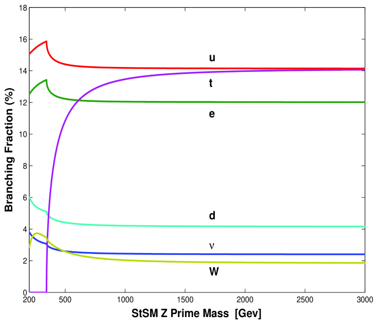
Figure 1: The StSM $Z^{\prime}$ branching ratios into $f\bar{f}$ and $W^{+}W^{-}$ final states as a function of the $Z^{\prime}$ mass with $f=u,t,e,d,\nu$ with $\epsilon=0.06$. Besides the exceptionally narrow total decay width, the large branching ratio of the StSM $Z^{\prime}$ into charged leptons further distinguishes this model from other $Z^{\prime}$ models.

in agreement with previous analyses of $Z^{\prime}$ decays [20, 21]. The $W^{+}W^{-}$ decay mode is suppressed by the small factor $R_{31}$, the element of the rotation matrix which indicates the mixing between $Z^{\prime}$ and $A^{3}$ gauge bosons. The $\Gamma(Z^{\prime}\rightarrow W^{+}W^{-})$ width is typically small relative to $\Gamma(Z^{\prime}\rightarrow\sum_{i}f_{i}\bar{f}_{i})$. It will be shown in the following sections that $\epsilon$ is severely limited by the electroweak constraints which leads to a Stueckelberg $Z^{\prime}$ resonance with a very narrow decay width. Thus the $Z^{\prime}$ decay width lies in the $\leq 100$ MeV range with $M_{Z^{\prime}}$ lying in the several hundred GeV to $1~{}\rm TeV$ range. In Fig. (1) it is shown that the $Z^{\prime}$ decays into quarks and leptons will dominate the total $Z^{\prime}$ decay width, as the $W^{+}W^{-}$ decay mode is roughly the same size as one species of $\nu\bar{\nu}$ mode. One may note that the branching ratio of $Z^{\prime}$ into the charged leptons is relatively large compared to what one has in conventional models. This is due to the StSM $Z^{\prime}$ couplings being dominated by the hypercharge of the particle in the final state. Thus, the isospin singlet $l_{R}$ which has a hypercharge $Y=-2$ contributes a significant amount which makes the charged lepton contribution comparable to the up quark contribution overcoming the color factor. The above also indicates that this $Z^{\prime}$ model can be efficiently tested in an $e^{+}e^{-}$ collider with polarized beams where one could check on the $l_{R}$ vs $l_{L}$ couplings. Such an experiment will be possible at the ILC. The above, coupled with the Drell-Yan analysis is a prime example of the physics interplay between the ILC and LHC [48].

3 The Stueckelberg Extension of LR Symmetric Models

3.1 Mass Matrix and Interactions

Next we discuss the Stueckelberg extension of the Left-Right Symmetric model (abbreviated by StLR) introduced in [4]. The gauge sector of this group is given by $SU(2)_{L}\times SU(2)_{R}\times U(1)_{B-L}\times U(1)_{X}$ with gauge bosons $A^{a\mu}_{L},A^{a\mu}_{R},B^{\mu},C^{\mu}$. As in LR models we assume the Higgs sector of the model to include $SU(2)_{L}$ and $SU(2)_{R}$ doublets $\Phi_{L,R}$ and a $SU(2)_{L}\times SU(2)_{R}$ bi-doublet $\xi$. We take the Lagrangian for the extended model to be

$$\mathcal{L}_{\rm StLR}=\mathcal{L}_{\rm St}+\mathcal{L}_{\rm LR},$$ (20)

where $\mathcal{L}_{\rm St}$ is the same as in StSM and is given by Eq. (3), and where $\mathcal{L}_{\rm LR}$ is the standard Left Right Symmetric Lagrangian [22] which we display below to define notation

$$\mathcal{L}_{\rm LR} = -\frac{1}{2}{\rm Tr}\left(F_{L\mu\nu}F_{L}^{\mu\nu}\right)-\frac{1}{2}{\rm Tr}\left(F_{R\mu\nu}F_{R}^{\mu\nu}\right)-\frac{1}{4}B_{\mu\nu}B^{\mu\nu}$$

$$+gA_{L\mu}^{a}\mathcal{J}_{2L}^{a\mu}+gA_{R\mu}^{a}\mathcal{J}_{2R}^{a\mu}+g^{\prime}B_{\mu}\mathcal{J}_{B-L}^{\mu}-\left(D^{\mu}\Phi_{L}\right)^{\dagger}D_{\mu}\Phi_{L}$$

$$-\left(D^{\mu}\Phi_{R}\right)^{\dagger}D_{\mu}\Phi_{R}-{\rm Tr}\left[\left(D^{\mu}\xi\right)^{\dagger}\left(D_{\mu}\xi\right)\right]-V\left(\Phi_{L},\Phi_{R},\xi\right).$$

We work with the manifest L-R symmetry $g=g_{2L}=g_{2R}$, and we use the notation $g^{\prime}=g_{BL}$. The set of Higgs multiplets under one pattern of symmetry breaking takes the form $\langle\Phi_{L}\rangle=v_{L}/\sqrt{2}$, $\langle\Phi_{R}\rangle=v_{R}/\sqrt{2}$, and

$$\langle\xi\rangle=\frac{1}{\sqrt{2}}\left(\begin{array}[]{cc}\kappa&0\\ 0&\kappa^{\prime}\end{array}\right),$$ (22)

with $\kappa^{\prime}\ll\kappa\ll v_{R}$, $v_{L}v_{R}=\gamma\kappa^{2}$ and $\gamma$ being the ratio of Higgs-particle self-couplings [22]. The mass squared matrix in the neutral sector is given by

$${M}_{{\rm StLR}}^{2}=\left(\begin{array}[]{cccc}M_{1}^{2}&M_{1}M_{2}&0&0\\ M_{1}M_{2}&\frac{1}{4}\left(v_{L}^{2}+v_{R}^{2}\right)g^{\prime 2}+M_{2}^{2}&-\frac{1}{4}gg^{\prime}v_{L}^{2}&-\frac{1}{4}gg^{\prime}v_{R}^{2}\\ 0&-\frac{1}{4}gg^{\prime}v_{L}^{2}&\frac{1}{4}g^{2}\left(v_{L}^{2}+\kappa^{2}+\kappa^{\prime 2}\right)&-\frac{1}{4}g^{2}\left(\kappa^{2}+\kappa^{\prime 2}\right)\\ 0&-\frac{1}{4}gg^{\prime}v_{R}^{2}&-\frac{1}{4}g^{2}\left(\kappa^{2}+\kappa^{\prime 2}\right)&\frac{1}{4}g^{2}\left(v_{R}^{2}+\kappa^{2}+\kappa^{\prime 2}\right)\end{array}\right)$$ (23)

which enters in the Lagrangian through

$$\mathcal{L}_{{\rm StLR}}\supset-\frac{1}{2}\tilde{\mathcal{V}}_{\mu}^{T}{M}_{{\rm StLR}}^{2}\tilde{\mathcal{V}}^{\mu}\hskip 14.22636pt{\rm with}\hskip 14.22636pt\tilde{\mathcal{V}}_{\mu}^{T}=(C_{\mu},B_{\mu},A_{L\mu}^{3},A_{R\mu}^{3}).$$ (24)

The matrix of Eq. (23) contains a massless mode, i.e. the photon, and three massive modes $Z,Z^{\prime},Z^{\prime\prime}$. We arrange the eigenvalues of ${M}_{{\rm StLR}}^{2}$ in the order

$${M}_{{\rm StLR-diag}}^{2}={\rm diag}\left(M_{Z^{\prime}}^{2},M_{Z}^{2},0,M_{Z^{\prime\prime}}^{2}\right),$$ (25)

with the corresponding eigenvectors

$$\tilde{\mathcal{E}}^{T}_{\mu}=\left(Z^{\prime}_{\mu},Z_{\mu},A^{\gamma}_{\mu},Z^{\prime\prime}_{\mu}\right),$$ (26)

where $\tilde{\mathcal{V}}^{\mu}$ and $\tilde{\mathcal{E}}^{\mu}$ are related by $\tilde{\mathcal{V}}^{\mu}=\mathcal{O}\tilde{\mathcal{E}}^{\mu}$, where $\mathcal{O}$ is an orthogonal matrix, $\mathcal{O}^{T}\mathcal{O}=I$. In our notation $A^{\gamma}_{\mu},Z_{\mu},Z_{\mu}^{{}^{\prime\prime}}$ are the usual modes in the LR model and $Z^{\prime}_{\mu}$ is the new mode arising due to mixing with the Stueckelberg sector. In this model the neutral current interactions have the form

$$g_{M}\sum\limits_{f}{\bar{f}}\gamma^{\mu}[(v_{f}-\gamma_{5}a_{f}){Z}_{\mu}+(v^{\prime}_{f}-\gamma_{5}a^{\prime}_{f})Z^{\prime}_{\mu}]f+eA_{\mu}^{\gamma}\left(\mathcal{J}_{B-L}^{\mu}+\mathcal{J}_{2L}^{3\mu}+\mathcal{J}_{2R}^{3\mu}\right)$$ (27)

where $e$ is given by

$$\frac{1}{e^{2}}=\frac{1}{g^{2}}(1-\epsilon^{2})+\frac{1}{g_{Y}^{2}}(1+\epsilon^{2})$$ (28)

and where $g_{Y}$ is related to $g=g_{2L}=g_{2R}$ and $g_{BL}=g^{\prime}$ by ${1}/{g_{Y}^{2}}={1}/{g^{2}}+{1}/{g^{2}_{BL}}$. The above relations limit to the standard LR relation as $\epsilon={M_{2}}/{M_{1}}\to 0$.

The vector and axial vector couplings of $Z$ and $Z^{\prime}$ to the matter fields are determined as in Section 2.2 and are,

$$\begin{array}[]{l}v_{f}=\frac{1}{\sqrt{g_{2}^{2}+g_{Y}^{2}}}[g({\mathcal{O}}_{32}+{\mathcal{O}}_{42})T^{3}_{f}+g^{\prime}{\mathcal{O}}_{22}(B-L)_{f}]\\ a_{f}=\frac{1}{\sqrt{g_{2}^{2}+g_{Y}^{2}}}[g({\mathcal{O}}_{32}-{\mathcal{O}}_{42})T^{3}_{f}],\\ \end{array}$$ (29)

$$\begin{array}[]{l}v^{\prime}_{f}=\frac{1}{\sqrt{g_{2}^{2}+g_{Y}^{2}}}[g({\mathcal{O}}_{31}+{\mathcal{O}}_{41})T^{3}_{f}+g^{\prime}{\mathcal{O}}_{21}(B-L)_{f}]\\ a^{\prime}_{f}=\frac{1}{\sqrt{g_{2}^{2}+g_{Y}^{2}}}[g({\mathcal{O}}_{31}-{\mathcal{O}}_{41})T^{3}_{f}].\\ \end{array}$$ (30)

The StLR $Z^{\prime}$ and StSM $Z^{\prime}$ share remarkably similar properties. A comparison between these two models is exhibited in Table (2). The analysis shows the interesting phenomenon that although the maximum allowed value of $\epsilon$ in the StLR is somewhat larger than in the StSM, the constraints on the axial-vector and vector couplings of the $Z^{\prime}$ with quarks and leptons and on the couplings with $W^{+}W^{-}$ are very similar to those in StSM. Consequently the branching ratios of the $Z^{\prime}$ into these modes are very similar. Thus as in the case of the StSM, one also finds that in the StLR, the dominant contribution to the decay of the $Z^{\prime}$ is from the quark and lepton final states. Restrictions on the parameter space of the limiting form of the StLR, which is the LR model, show that the decay into the extra heavy $W^{+}W^{-}$ final state is not kinematically allowed.

4 Constraints on the $U(1)_{X}$ Extensions

4.1 Constraint from the Correction to the $Z$ Mass

We use the variational technique of Ref. [23] to derive the shift on the $Z$ mass due to the effect of mixing with $C_{\mu}$. In general, for a real symmetric $n\times n$ matrix, the eigenvalue equation is an $n^{\rm th}$ order polynomial in $\lambda$

$$F(\lambda)=\sum\limits_{k=1}^{n}{C^{(k)}}{\lambda}^{k}=0.$$ (31)

The correction to an eigenvalue $\lambda_{i}$ due to a set of perturbation $\delta_{k}$ may be written as

$$\Delta\lambda_{i}=\sum\limits_{k=1}^{m}{\delta_{k}\frac{{\partial\lambda_{i}}}{{\partial\delta_{k}}}}=-\sum\limits_{k=1}^{m}{\delta_{k}\left({\frac{{\partial_{\delta_{k}}F}}{{\partial_{\lambda}F}}}\right)_{\lambda=\lambda^{*}_{ik}}},$$ (32)

where $\lambda^{*}_{ik}=\lim_{\delta_{k}\to 0}\lambda_{i}$. For the $U(1)_{X}$ extended theory we have after factoring out the zero eigenvalue the equation $F(\lambda)=C^{(2)}\lambda^{2}+C^{(1)}\lambda+C^{(0)}$ with

$$\begin{array}[]{l}C^{(2)}=1\\ C^{(1)}=-(M^{2}_{0}+M^{2}_{1}+M^{2}_{2})\\ C^{(0)}=M^{2}_{1}M^{2}_{0}+M^{2}_{0}M^{2}_{2}c^{2}_{W},\end{array}$$ (33)

where we are interested in the shift on the $Z$ mass (as given by Eq. (2.1)) due to the perturbation $\delta=M^{2}_{2}$. The above gives

$$\Delta M_{Z}\approx-\frac{1}{2}M_{0}s^{2}_{W}(1-{M_{0}^{2}}/{M_{1}^{2}})^{-1}\epsilon^{2}.$$ (34)

To determine the allowed corridors in $\epsilon$ and $M_{1}$, we follow a similar approach as in the analysis of Refs. [24, 25] used in constraining the size of extra dimensions. We begin by recalling that in the on-shell scheme the $W$ boson mass including loop corrections becomes [26]

$${M}_{W}^{2}\to\frac{\pi\alpha}{\sqrt{2}G_{F}s^{2}_{W}(1-\Delta r)},$$ (35)

where the Fermi constant $G_{F}$ and the fine structure constant $\alpha$ (at $Q^{2}=0$) are known to a high degree of accuracy. The quantity $\Delta r$ is the radiative correction and is determined so that $\Delta r=0.0363\pm 0.0019$ [27], where the uncertainty comes from error in the top mass and from the error in $\alpha(M_{Z}^{2})$. Since in the on-shell scheme $s^{2}_{W}=(1-M_{W}^{2}/M_{Z}^{2})$ one may use Eq. (35) and the current experimental value of $M_{W}=80.425\pm 0.034$ [27] to make a prediction of $M_{Z}$. Such a prediction within the SM is in excellent agreement with the current experimental value of $M_{Z}=91.1876\pm 0.0021$. Thus the above analysis requires that the effects of the Stueckelberg extension on the $Z$ mass must be such that they lie in the error corridor of the SM prediction. From Eq. (35) we find

$$\delta M_{Z}=M_{Z}\sqrt{\left(\frac{1-2\sin^{2}\theta_{W}}{\cos^{3}\theta_{W}}\frac{\delta M_{W}}{M_{Z}}\right)^{2}+\frac{\tan^{4}\theta_{W}(\delta\Delta r)^{2}}{4(1-\Delta r)^{2}}}.$$ (36)

Equating the StSM shift of the $Z$ mass, Eq. (34), in the region $M_{1}^{2}\gg M_{Z}^{2}$, to the SM error corrider of the $Z$ mass, Eq. (36), one finds an upper bound on $\epsilon$ [4]

$$|\epsilon|\lesssim.061\sqrt{1-(M_{Z}/M_{1})^{2}}.$$ (37)

4.2 Constraints from Other Precision Electroweak Data

Next we investigate the implications of the previous analysis on the precisely determined observables in the electroweak sector. We follow closely the analysis of the LEP Working Group [27] (see also Refs. [28, 29]), except that we will use the vector ($v_{f}$) and the axial vector ($a_{f}$) couplings for the fermions in the StSM. The couplings of the $Z$ to the fermions in the StSM are elevated from the tree level expressions of Eqs. (11) to

$$\begin{array}[]{l}v_{f}=\sqrt{\rho_{f}}[(c_{W}R_{32}-s_{W}R_{22})T^{3}_{f}+2\kappa_{f}Q_{f}s_{W}R_{22}]\\ a_{f}=\sqrt{\rho_{f}}(c_{W}R_{32}-s_{W}R_{22})T^{3}_{f},\\ \end{array}$$ (38)

where $\rho_{f}$ and $\kappa_{f}$ (in general complex valued quantities) contain radiative corrections from propagator self energies and flavor specific vertex corrections and are as defined in Refs. [30, 27]. The decay of the $Z$ boson into lepton anti-lepton and quark anti-quark pairs (excluding the top) in the on-shell renormalization scheme is given by [28, 30]

$$\Gamma(Z\to f\bar{f}) = N_{f}^{c}\mathcal{R}_{f}\Gamma_{o}\sqrt{1-4\mu_{f}^{2}}\Bigg{[}|v_{f}|^{2}(1+2\mu_{f}^{2})+|a_{f}|^{2}(1-4\mu_{f}^{2})\Bigg{]},$$ (39)

$$\mathcal{R}_{f} = \left(1+\delta_{f}^{QED}\right)\left(1+\frac{N_{f}^{c}-1}{2}\delta_{f}^{QCD}\right),$$ (40)

$$\delta_{f}^{QED} = \frac{3\alpha}{4\pi}Q_{f}^{2},$$ (41)

$$\delta_{f}^{QCD} = \frac{{\alpha_{s}}}{\pi}+1.409\left({\frac{{\alpha_{s}}}{\pi}}\right)^{2}-12.77\left({\frac{{\alpha_{s}}}{\pi}}\right)^{3}-Q_{f}^{2}\frac{{\alpha\alpha_{s}}}{{4\pi^{2}}}.$$ (42)

Here $\alpha$ and $\alpha_{s}$ are taken at the $M_{Z}$ scale, while $N_{f}^{c}=(1,3)$ for leptons and quarks. In the above, $\Gamma_{o}=G_{F}M^{3}_{Z}/6\sqrt{2}\pi$, and $\mu_{f}=m_{f}/M_{Z}$. The total decay width ($\Gamma_{Z}$) of the $Z$ into quarks and leptons, in the visible sector, is just the sum over all the final states.

We also investigate the effects of mixing with the Stueckelberg sector on the following $Z$ pole observables

$$R_{l} = \frac{\Gamma(had)}{\Gamma(l^{+}l^{-})},$$ (43)

$$R_{q} = \frac{\Gamma(q\bar{q})}{\Gamma(had)},$$ (44)

$$\sigma_{had} = \frac{12\pi\Gamma(e^{+}e^{-})\Gamma(had)}{M_{Z}^{2}\Gamma_{Z}^{2}},$$ (45)

$$A_{f} = \frac{2v_{f}a_{f}}{v^{2}_{f}+a^{2}_{f}},$$ (46)

$$A^{(0,f)}_{FB} = \frac{3}{4}A_{e}A_{f}.$$ (47)

Using the above we have carried out a fit in the electroweak sector on the quantities sensitive to mixing with the Stueckelberg sector. A summary of the analysis is presented in Table (1) for $M_{1}=350$ GeV and $\epsilon$ lying in the range (0.035-0.059). The analysis of Pulls in Table (1) indicates that the fits are excellent. Indeed for the case $\epsilon=.035$, the StSM gives essentially the same $\chi^{2}$ fit to data as the SM. For the case $\epsilon=0.059$ the Pulls are again of the same quality as for the SM when $A_{FB}^{(0,b)}$ is excluded but somewhat larger when $A_{FB}^{(0,b)}$ is included. However, $A_{FB}^{(0,b)}$ is known to be problematic even in the SM. Thus, for example, $A_{FB}^{(0,b)}$ lies in the range [-2.5,-2.8] in the analysis of Ref. [27] and it is implied that the significant shift could be the result of fluctuations in experimental measurements. It is similarly stated in Ref. [30] that at least a part of the problem in this case may be experimental. The above appears to indicate that $A_{FB}^{(0,b)}$ is on a somewhat less firm footing than the other electroweak parameters. The constraints on the $Z^{\prime}$ of StLR are very similar to the constraints on the $Z^{\prime}$ arising in StSM and we do not give a separate detailed analysis of it here.

5 Comparison of the Stueckelberg $Z^{\prime}$ and Classic $Z^{\prime}$ Models

5.1 The Stueckelberg $Z^{\prime}$ and the CDDT Parametrization

It is instructive to compare the Stueckelberg $Z^{\prime}$ model with other $Z^{\prime}$ models. For this purpose it is convenient to use the parametrization of the orthogonal matrix $R$ in terms of angles [3]

$${R}=\left(\begin{array}[]{ccc}c_{\psi}c_{\phi}-s_{\theta}s_{\phi}s_{\psi}&-s_{\psi}c_{\phi}-s_{\theta}s_{\phi}c_{\psi}&-c_{\theta}s_{\phi}\\ c_{\psi}s_{\phi}+s_{\theta}c_{\phi}s_{\psi}&-s_{\psi}s_{\phi}+s_{\theta}c_{\phi}c_{\psi}&c_{\theta}c_{\phi}\\ -c_{\theta}s_{\psi}&-c_{\theta}c_{\psi}&s_{\theta}\end{array}\right),$$ (48)

where

$$\tan(\phi)=\frac{M_{2}}{M_{1}}=\epsilon,\hskip 14.22636pt\tan(\theta)=\frac{g_{Y}}{g_{2}}\cos(\phi)=\tan\left(\theta_{W})\right.\cos(\phi),$$ (49)

$$\tan(\psi)=\frac{\tan(\theta)\tan(\phi)M_{W}^{2}}{\cos(\theta)\left(M_{Z^{{\prime}}}^{2}-M_{W}^{2}\left(1+\tan^{2}(\theta)\right)\right)}.$$ (50)

The SM limit, again, corresponds to $\epsilon\to 0$ which implies $\tan(\phi),~{}\tan(\psi)\to 0$ and $\theta\to\theta_{W}$. Using Eq. (48) we may write the photon field $A_{\mu}^{\gamma}$ in the form

$$A^{\gamma}_{\mu}=-c_{\theta}s_{\phi}C_{\mu}+c_{\theta}c_{\phi}B_{\mu}+s_{\theta}A^{3}_{\mu},$$ (51)

which shows that the photon field contains a component outside of the set $(B_{\mu},~{}A^{3}_{\mu})$ while in the conventional $Z-Z^{\prime}$ models the photon field is just a linear combination of the fields $(B_{\mu},~{}A^{3}_{\mu})$. This is what sets the StSM model apart from the conventional models. To carry out the comparison with the $Z-Z^{\prime}$ models a bit further we might try to mimic the $Z-Z^{\prime}$ models by introducing “ rotated fields ” $\tilde{B}^{\mu}_{Y}$ and $\tilde{C}^{\mu}$

$$\tilde{B}^{\mu}_{Y} = B^{\mu}\cos\phi-C^{\mu}\sin\phi$$

$$\tilde{C}^{\mu} = B^{\mu}\sin\phi+C^{\mu}\cos\phi,$$ (52)

where the rotation depends only on $\epsilon$. In terms of new variables the physical vector fields in StSM are

$$A^{\mu}_{\gamma} = W^{3\mu}\sin\theta+\tilde{B}^{\mu}_{Y}\cos\theta$$

$$Z^{\mu} = (W^{3\mu}\cos\theta-\tilde{B}^{\mu}_{Y}\sin\theta)\cos\psi+\tilde{C}^{\mu}\sin\psi$$

$$Z^{\prime\mu} = \tilde{C}^{\mu}\cos\psi-(W^{3\mu}\cos\theta-\tilde{B}^{\mu}_{Y}\sin\theta)\sin\psi,$$ (53)

where $W^{3\mu}\equiv A^{3\mu}$. The mass terms for a generic $Z-Z^{\prime}$ mixing model with the gauge group $SU(2)_{L}\times U(1)_{Y}\times U(1)_{Z}$ are typically given by [18]

$$\frac{v_{H_{1}}^{2}}{8}(gW^{3\mu}-g_{Y}B^{\mu}-z_{H_{1}}g_{Z}B_{Z}^{\mu})^{2}+\frac{v_{H_{2}}^{2}}{8}(gW^{3\mu}-g_{Y}B^{\mu}-z_{H_{2}}g_{Z}B_{Z}^{\mu})^{2}+\frac{v_{\phi}^{2}}{8}(z_{\phi}g_{Z}B_{Z}^{\mu})^{2}$$ (54)

where $g_{Z}$ is the $U(1)_{Z}$ gauge coupling constant and $B_{Z}^{\mu}$ is used to denote the $U(1)_{Z}$ gauge field. Here the eigenvectors for the photon, $Z$ and $Z^{\prime}$ are as follows

$$A^{\mu}_{\gamma} = W^{3\mu}\sin\theta_{W}+B^{\mu}\cos\theta_{W}$$

$$Z^{\mu} = (W^{3\mu}\cos\theta_{W}-B^{\mu}\sin\theta_{W})+\epsilon_{Z}B^{\mu}_{Z}$$

$$Z^{\prime\mu} = B^{\mu}_{Z}-\epsilon_{Z}(W^{3\mu}\cos\theta_{W}-B^{\mu}\sin\theta_{W})$$ (55)

where

$$\epsilon_{Z}=\frac{\delta M^{2}_{ZZ^{\prime}}}{M_{Z^{\prime}}^{2}-M_{Z}^{2}},$$ (56)

and where $M_{Z}$, $M_{Z^{\prime}}$ and $\delta M^{2}_{ZZ^{\prime}}$ are given by

$$M_{Z}^{2} = \frac{g^{2}(v_{H_{1}}^{2}+v_{H_{2}}^{2})}{4\cos^{2}\theta_{W}}[1+O(\epsilon^{2}_{Z})]$$

$$M_{Z^{\prime}}^{2} = \frac{g^{2}_{Z}}{4}(z_{H_{1}}^{2}v_{H_{1}}^{2}+z_{H_{2}}^{2}v_{H_{2}}^{2}+z_{\phi}^{2}v_{\phi}^{2})[1+O(\epsilon^{2}_{Z})]$$

$$\delta M^{2}_{ZZ^{\prime}} = -\frac{gg_{Z}}{4\cos\theta_{W}}(z_{H_{1}}v_{H_{1}}^{2}+z_{H_{2}}v_{H_{2}}^{2}).$$ (57)

Using the rotated fields one finds that there is some similarity between the expressions for the physical fields in Eq. (53) and in Eq. (55). However, this similarity is superficial and a closer scrutiny of the mass matrices reveals that there is no limiting procedure connecting the sets of expressions. Of course this should be rather obvious since the symmetry breaking in the $Z-Z^{\prime}$ models arises only from the Higgs sector while in StSM such a breaking arises both from the Higgs sector and from the Stueckelberg sector. Further, in $Z-Z^{\prime}$ analyses $\epsilon_{Z}$ is severely constrained by LEP data ( $|\epsilon_{Z}|\lesssim 10^{-3}$) and is either neglected [18, 31] in the diagonalizaton procedure or the case considered is $z_{H_{2}}=0$ with $\tan\beta=v_{H_{2}}/v_{H_{1}}\gtrsim 10$ . In either case, these extensions do not allow for narrow resonances of MeV size widths. The mass matrix given in Eq. (5) is also valid for the minimal Stueckelberg Supersymmetric Standard Model [StMSSM] [2]. Some of the experimental implications of StSM and of StMSSM particularly with regard to the $e^{+}e^{-}$ colliders were investigated in Ref. [3]. However, the implications at hadron colliders and specifically at the LHC were not discussed and this is the main topic of discussion in this paper. In summary the Stueckelberg extended models form a new class outside the framework of the usual $Z-Z^{\prime}$ mixing models given generically by Eqs. (54-57) and there is no limiting procedure connecting these models with the StSM.

6 LHC Observables and Constraints on the StSM Parameter Space

6.1 Drell-Yan Cross Section for $pp\to Z^{\prime}\to l^{+}l^{-}$

Next we discuss the production of the narrow $Z^{\prime}$ by the Drell-Yan process at the LHC. For the hadronic process $A+B\to V+X$, and the partonic subprocess $q\bar{q}\to V\to l^{+}l^{-}$, the dilepton doubly differential cross section to next to leading order (NLO) is given by

$$\frac{{d^{2}\sigma_{{{AB}}}}}{{dM^{2}dz}}=K\frac{1}{s}\sum\limits_{q}{\left[{\frac{d\sigma_{q\bar{q}}^{SM}}{{dz}}}+{\frac{d\sigma_{q\bar{q}}^{St-SM}}{{dz}}}+{\frac{d\sigma_{q\bar{q}}^{St}}{{dz}}}\right]}{\mathcal{W}}_{\left\{{{AB}(q\bar{q})}\right\}}(s,M^{2}).$$ (58)

$$\mathcal{W}_{\left\{{AB}\left(q\bar{q}\right)\right\}}(\tau)=\int_{0}^{1}\int_{0}^{1}dxdy\delta(\tau-xy)\mathcal{P}_{\left\{{AB}\left(q\bar{q}\right)\right\}}(x,y),$$

$$\mathcal{P}_{\left\{{AB}\left(q\bar{q}\right)\right\}}(x,y)=f_{q,A}(x)f_{\bar{q},B}(y)+f_{\bar{q},A}(x)f_{q,B}(y).$$ (59)

Here the dimensionless variable $\tau=M^{2}/s$ relates the invariant mass $M$ of the final state lepton pair to the center of mass energy $\sqrt{s}$ of the colliding hadrons and $z=\cos{\theta^{*}}$, where $\theta^{*}$ is the angle between an initial state parton and the final state lepton in the C-M frame of the lepton anti-lepton pair. The term $d\sigma^{SM}/dz$ is the Standard Model contribution, $d\sigma^{St}/dz$ is the contribution from the Stueckelberg sector, and $d\sigma^{St-SM}/dz$ is the interference term between the Standard Model and the Stueckelberg sectors. The parton distribution functions (PDFs) which we denote by $f_{q,A}(x)$ give the probability that a parton of type $q$ has a fracton $x$ of the total hadron four momentum. The dependence of $f_{q,A}(x)$ on the mass factorization scale $Q=M$ is implicit. For the LHC $A=B=p$, and one must note that quite generally that $f_{q,A}=f_{\bar{q},\bar{A}}$ and $f_{\bar{q},A}=f_{q,\bar{A}}$. The Drell-Yan $K$ factor is as discussed in detail in Refs. [32, 18, 16, 28, 34]. The invariant dilepton differential cross section is at NLO

$$\frac{d\sigma_{AB}}{dM}=K\frac{2M}{s}\sum_{q}\sigma_{q\bar{q}}\left(M^{2}\right)\mathcal{W}_{\left\{{AB}\left(q\bar{q}\right)\right\}}(\tau),$$ (60)

where the partonic cross section, ${\sigma}_{q\bar{q}}$, is defined by integrating the term in square brackets of Eq. (58) over the variable $z$ and is computed in Ref. [3]. While $d\sigma/dM$ is sensitive to the interference term, the integral over $dM$ is not. Thus for the computation of $d\sigma/dz$ one may just use the $Z^{\prime}$ pole contribution in Eq. (58). Using the analysis of Ref.[3] for the partonic process $q\bar{q}\to l^{+}l^{-}$ one finds that for $pp$ collisions the integration of the third term of Eq. (58) over $M^{2}$ yields the angular distribution for the StSM $Z^{\prime}$ model

$$\frac{{d\sigma_{{{AB}}}}}{{dz}}=\frac{K}{s}\sum\limits_{q}{\mathcal{W}}_{\left\{{{AB}(q\bar{q})}\right\}}(s,M^{2}_{Z^{\prime}})\frac{G_{F}^{2}M_{Z}^{4}M_{Z^{\prime}}}{48\Gamma_{Z^{\prime}}}\left[(1+z^{2})(a_{e}^{\prime 2}+v_{e}^{\prime 2})(a_{q}^{\prime 2}+v_{q}^{\prime 2})\right].$$ (61)

A further integration over $z$ gives the production cross section for the Stueckelberg $Z^{\prime}$ gauge boson

$$\sigma_{AB}\cdot Br(Z^{\prime}\to l^{+}l^{-})=K\frac{\pi}{{6s}}\sum\limits_{q}{C_{q}}{\mathcal{W}}_{\left\{{{AB}(q\bar{q})}\right\}}(s,M_{Z^{\prime}}^{2}),$$ (62)

where dimensionless $C_{q}$ are given by

$$C_{q}=2g_{M}^{2}Br(Z^{\prime}\to l^{+}l^{-})(a^{\prime 2}_{q}+v^{\prime 2}_{q}),\hskip 14.22636ptq=u,d$$ (63)

and where $g_{M}^{2}=\sqrt{2}G_{F}M_{Z}^{2}$. The $C_{u}-C_{d}$ parameterization is as defined in Ref. [18] and allows one to use experimental limits set on the dilepton final state production cross section without making reference to the PDFs; the couplings of a particular model are needed only, if the experimental limits are known. In fact, such a paramerization is perhaps the first step in solving the potential ”LHC inverse problem” [35] for the case of the $Z^{\prime}$ as one can directly map between the signature space and the parameter space in a very simple way. The relation between $C_{u}$ and $C_{d}$ is

$$\frac{C_{u}}{C_{d}}=\frac{(v^{\prime 2}_{u}+a^{\prime 2}_{u})}{(v^{\prime 2}_{d}+a^{\prime 2}_{d})}\sim\frac{\mbox{Br}(Z^{\prime}\rightarrow u\bar{u})}{\mbox{Br}(Z^{\prime}\rightarrow d\bar{d})}.$$ (64)

Although $C_{(u,d)}$ are functions of $\epsilon$ for the StSM, the ratio is in fact independant of $\epsilon$. The formulas given in this section are also valid for the case of the StLR via transcribing the couplings as laid out in Eq. (30).

6.2 Constraints on the StSM Parameter Space from the CDF and DØ Data

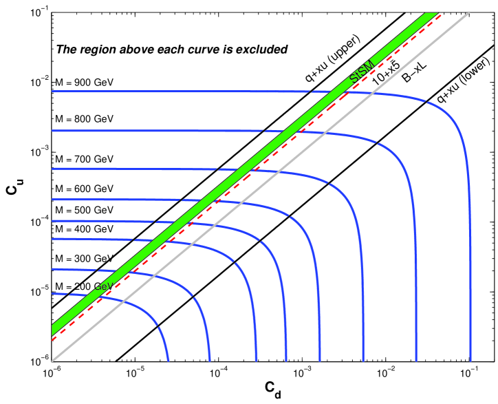
Figure 2: Excluded regions in the $C_{u}-C_{d}$ plane from the current 95% C.L. limit for $\sigma\cdot\mbox{Br}(Z^{\prime}\rightarrow l^{+}l^{-})$ given in [36] at 819 ${\rm pb}^{-1}$ for different $Z^{\prime}$ masses, labeled as $M$ in the figure. The shaded green band is the region where the StSM model lies and where $2.49C_{d}<C_{u}<3.37C_{d}$. The light straight line corresponds to $C_{u}$ and $C_{d}$ in the $B-xL$ model where $C_{u}=C_{d}$ (see [18]). The area between the two black straight lines is the region where the $q+xu$ model lies and where $(3-2\sqrt{2})C_{d}<C_{u}<(3+2\sqrt{2})C_{d}$. The $10+x\bar{5}$ model is constrained below the dashed red line which corresponds $C_{u}=2C_{d}$.

As discussed above the $C_{u}$-$C_{d}$ parametrization [18] provides a useful technique to explore the limits on new physics and allows one to distinguish among various classes of models. For instance, in the $C_{u}-C_{d}$ plane the $C_{u}$ and $C_{d}$ predicted in the StSM lie inside a band. The band structure for StSM arises since the ratio $C_{u}/C_{d}$ as given by Eq. (64) lies in the range 2.49 $\sim$ 3.37 for $M_{Z^{\prime}}$ lying in the range $200\sim 900$ GeV. Similarly, the $C_{u}$ and $C_{d}$ predicted in the $q+xu$ model [18] also lie in a band, while the $C_{u}$ and $C_{d}$ for the $B-xL$ model [18] live on a line. In Fig. (2) we give a numerical evaluation of the $C_{u}$ and $C_{d}$ using the most recent CDF data of 819 ${\rm pb}^{-1}$ in the dilepton channel [36]. The $C_{u}$-$C_{d}$ exclusion plots of Fig. (2) can be used to constrain $\epsilon$ for a given $M_{Z^{\prime}}$. These constraints are consistent with the constraints derived using a smaller data sample of approxomately 275 ${\rm pb}^{-1}$ which, however, uses the more sensitive DØ mode [37]. In addition to the above one also has constraints on the parameter space from the non-observation of the $Z^{\prime}$ from the CDF and DØ data [36, 37, 38, 39]. These constraints were shown to limit values of $(\epsilon,M_{Z^{\prime}})$ in [4], while still allowing for the possibility of a narrow StSM $Z^{\prime}$ which could even lie relatively close to the $Z$-pole.

7 Discovery Reach of LHC for StSM $Z^{\prime}$ Boson

7.1 $\sigma\cdot Br(Z^{\prime}\to l^{+}l^{-})$ at the LHC

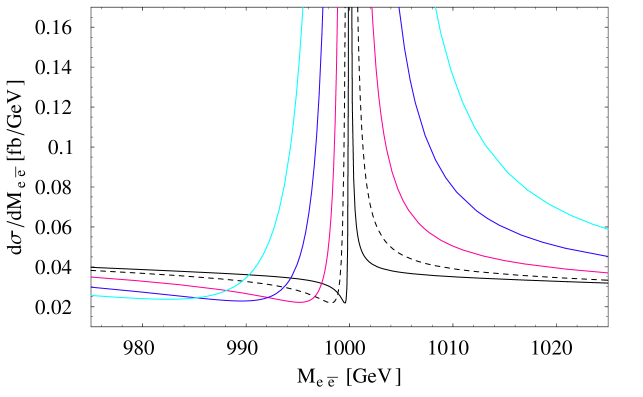
Figure 3: The invariant dilepton differential cross section, $d\sigma(pp\to Z^{\prime}\to l^{+}\l^{-})/dM$ as a function of the dilepton invariant mass for various $\epsilon$ values. The plot exhibits the narrow widths at the $Z^{\prime}$ pole. The dashed curve corresponds to $\epsilon=.06$. The shapes of these curves illustrate the exceptionally narrow resonance widths of the StSM $Z^{\prime}$ with distinct distributions.

Next we give an analysis for the exploration of the $Z^{\prime}$ boson at the LHC. Before proceeding further it is instructive to examine the shape of the $d\sigma/dM$ as a function of the invariant mass $M$. This is exhibited in Fig. (3) where the plots are given for an array of values of $\epsilon$ (ranging over the set $\{.03,.06,.1,.15,.2\}$ where the larger values of $\epsilon$ are taken only for illustrative purposes) for the case when $M_{1}=1$ TeV. One can appreciate the narrowness of the $Z^{\prime}$ pole from these plots. This type of shape and width is strikngly different from the ones encountered in the conventional $Z^{\prime}$ models [16] and also in Kaluza-Klein excitations of the $Z$ boson in large radius extra dimension models [40, 41].

The quantity that will be measured experimentally at the LHC is $\sigma_{pp}\cdot Br(X\to l^{+}l^{-})\equiv\sigma\cdot Br(X\to l^{+}l^{-})$ in the process $pp\to X\to l^{+}l^{-}$ where $X$ is a neutral resonant state produced in $pp$ collisions which can decay into a lepton pair. Here we give a theoretical analysis of this quantity for the case when $X=Z^{\prime}$, and in the next section we will consider the case when $X=G$, the spin 2 graviton of a warped geometry. In the analysis of $\sigma\cdot Br(Z^{\prime}\to l^{+}l^{-})$ we will discuss two regions: a low mass region with the dilepton invariant mass $M_{l\bar{l}}$ up to 800 GeV and a high mass region with $M_{l\bar{l}}$ extending from 800 GeV up to the maximum relevant mass reach of the LHC. The reason for this ordering is as follows: the region with $M_{l\bar{l}}$ up to 800 GeV has already begun to be explored at the Tevatron using up to about $1~{}\rm fb^{-1}$ of data, and the CDF and DØ data puts constraints on $\epsilon$ as a function of the dilepton invariant mass. Thus in the analysis of the low mass $M_{l\bar{l}}$ region at the LHC we can incorporate these constraints. However, one has no direct constraints in the dilepton invariant mass region above 800 GeV, which explains the separate analyses of $\sigma\cdot Br(Z^{\prime}\to l^{+}l^{-})$ for the low and high mass regions.

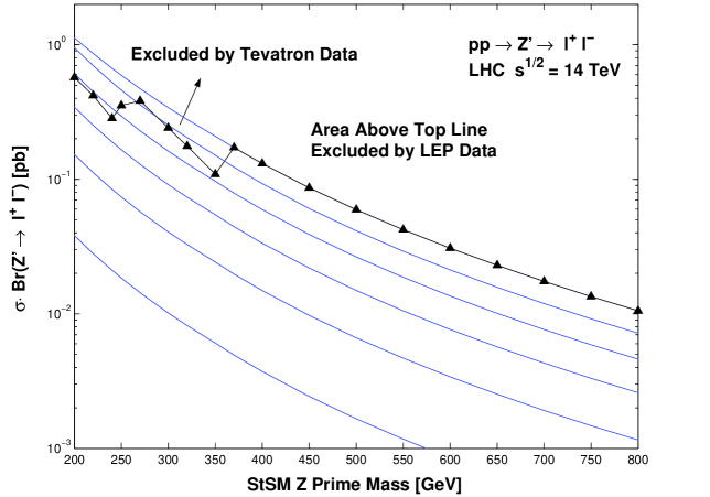
Figure 4: The production cross section $\sigma\cdot Br(Z^{\prime}\to l^{+}l^{-})$ [pb] in the StSM at the LHC in the low mass region with the inclusion of the LEP and Tevatron constraints. The curves in descending order correspond to values of $\epsilon$ from .06 to .01 in steps of .01.

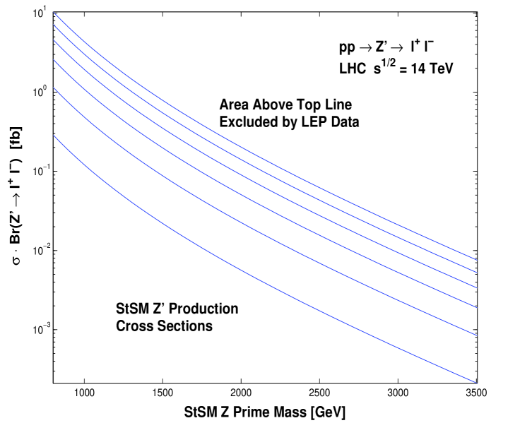
Figure 5: The production cross section $\sigma\cdot Br(Z^{\prime}\to l^{+}l^{-})$ [fb] in the StSM at the LHC in the $Z^{\prime}$ high mass region up to $Z^{\prime}$ mass of $\approx$ 3.5 TeV. The curves correspond to values of $\epsilon$ ranging from $.06$ to $.01$ in descending order in steps of .01. The StSM production cross sections sit several orders of magnitude below those of other $Z^{\prime}$ models.

We begin with an analysis of $\sigma\cdot Br(Z^{\prime}\to l^{+}l^{-})$ in the low mass region where we use the constraints on $(\epsilon,M_{Z^{\prime}})$ as obtained in Ref. [4] using the cross section limits from [37]. The results are displayed in Fig. (4). As expected one finds that the current data on $\sigma\cdot Br(Z^{\prime}\to l^{+}l^{-})$ constrains only the mass region of $Z^{\prime}$ for values $M_{Z^{\prime}}\lesssim 350$ GeV. We note that for $\epsilon$ as high as $\approx.04$ one may have an StSM $Z^{\prime}$ as low as 175 GeV, while with a $Z^{\prime}$ mass of 250 GeV, $\epsilon$ may be as high as $\approx.035$ within the current experimental limits. Next we discuss the high mass region for the StSM $Z^{\prime}$. As discussed above the high mass region of StSM $Z^{\prime}$ remains unconstrained by the CDF and DØ data, and thus in this region only the LEP electroweak constraints apply. The analysis of Fig. (5) gives a plot of $\sigma\cdot Br(Z^{\prime}\to l^{+}l^{-})$ as a function of $M_{Z^{\prime}}$ in the high mass region for values of $\epsilon$ ranging from $.01$ to $.06$ in ascending order in steps of $.01$. From Fig. (5) and from the analysis of Refs. [31, 42] for other $Z^{\prime}$ models one infers that the production cross section for StSM $Z^{\prime}$ lies orders of magnitude below those for the $Z^{\prime}$ production in E6 models and other $Z^{\prime}$ models. The size of $\sigma\cdot Br(Z^{\prime}\to l^{+}l^{-})$ thus provides a clear signature which differentiates the StSM $Z^{\prime}$ model from other $Z^{\prime}$ models.

7.2 Signal to Background Ratio

The dilepton channel will be analyzed at the LHC in the ATLAS [56] and CMS [57] detectors, and as is discussed below, both detectors have the ability to probe the narrow StSM $Z^{\prime}$ boson. Experimentally, the discovery of a narrow resonance depends to a significant degree on the bin size for data collection with the chance of detection increasing with a decreasing bin size. This is so because the integral over the bin is effectively independent of the bin size for the signal (assuming the narrow resonance falls within the bin). However, this integral is essentially linearly dependent on the bin size for the SM background. In the analysis of the SM background we have included the $Z,\gamma$, and $\gamma-Z$ interference terms in the Drell-Yan analysis, but have not included the backgrounds from other sources such as from $t\bar{t},b\bar{b},WW,WZ,ZZ$ etc. However, these backgrounds are known to be at best a few percent of the Drell-Yan background [63]. Regarding the bin size, it depends on the energy resolution $\sigma_{E}/E$ of the calorimeter. For an electromagnetic calorimeter the energy resolution is typically parameterized by $\sigma_{E}/E=a/\sqrt{E}\oplus b\oplus c/E$ where addition in quadrature is implied[67]. The term proportional to $1/\sqrt{E}$ is the so called stochastic term and arises from statistic related fluctuations. The term $b$ is due to detector non-uniformity and calibration errors, and the term $c$ is due mostly to noise. For the ATLAS detector (liquid Ar/Pb) the energy resolution is parameterized by [67] $\sigma_{E}=10\%/\sqrt{E}\oplus.4\%\oplus.3/E$ and for the CMS detector ($\rm PbWO_{4}$) it is parameterized by $\sigma_{E}=3\%/\sqrt{E}\oplus.5\%\oplus.2/E$ where $E$ is in units of GeV. From the above we find the following relations for the bin size B (taken to be 6$\sigma_{E}$) at the mass scale $M$ ($M$ is measured in units of TeV)

$${\rm B}_{\rm ATLAS}=24(.625M+M^{2}+.0056)^{1/2}{\rm GeV}$$

$${\rm B}_{\rm CMS}=30(.036M+M^{2}+.0016)^{1/2}{\rm GeV}.$$ (65)

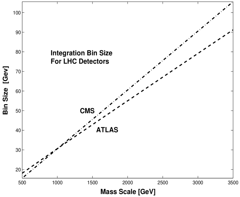
Figure 6: A plot of the mass window or bin size as a function of the mass scale for the ATLAS and CMS detectors.

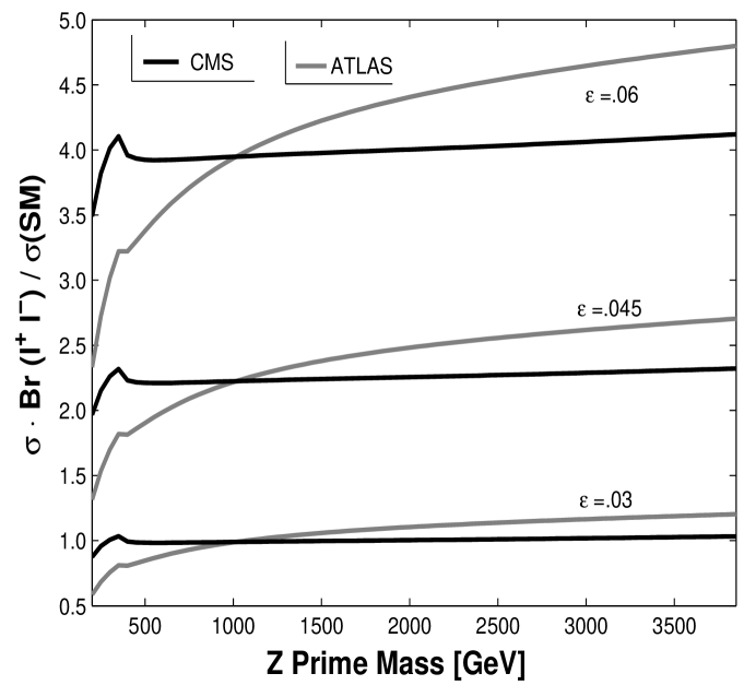
Figure 7: A plot of the ratio $\sigma\cdot Br(Z^{\prime}\to l^{+}l^{-})_{StSM}/\sigma_{SM}(Z,\gamma\to l^{+}l^{-})$ including the $\gamma-Z$ interference term in the SM as a function of the $Z^{\prime}$ mass for the ATLAS and CMS detectors assuming the bin sizes as in Fig.(6) for values of $\epsilon$ in the range .03-.06. The signal to background ratio is larger for the CMS detector at low mass scales while it is larger for the ATLAS detector at large mass scales with a cross over occuring at around 1 TeV.

For $M>3$ TeV, the $M^{2}$ term dominates in Eq.(65) and the bin size goes linearly in $M$, so ${\rm B}_{\rm ATLAS}\sim 24M$ GeV and ${\rm B}_{\rm CMS}\sim 30M$ GeV for large $M$. A plot of bin sizes as a function of the mass scale is given in Fig.(6) for the two LHC detectors. One finds that at low mass scales the CMS has a somewhat better energy resolution and thus a somewhat smaller bin sizes and at large mass scales ATLAS has a somewhat better energy resolution and thus a somewhat smaller bin size with a cross over at $M\sim 1$ TeV. However, on the whole the energy resolution and the bin size of the two detectors are comparable within about 10%. For the StSM $Z^{\prime}$ the analysis of Fig. (7) shows that the signal to background is greater than unity in significant parts of the parameter space, and in some cases greater than 4, thus illustrating that the LHC has the ability to detect a strong signal for a StSM $Z^{\prime}$.

7.3 How Large a $Z^{\prime}$ Mass and How Narrow a $Z^{\prime}$ Width Can LHC Probe?

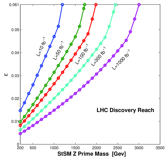
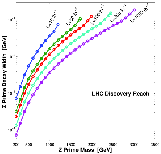
Figure 8: A plot of the discovery limits of $Z^{\prime}$ in StSM with the discovery limit defined by $5\sqrt{N_{SM}}$ or by 10 events, whichever is larger. The inflections, or kinks, in the plots are precisely the points of transitions between the two criteria. Regions to the left and above each curve can be probed by the LHC at a given luminosity. The top point on each curve corresponds to $\epsilon=.061$. The analysis is done for the ATLAS detector but similar results hold for the CMS detector.

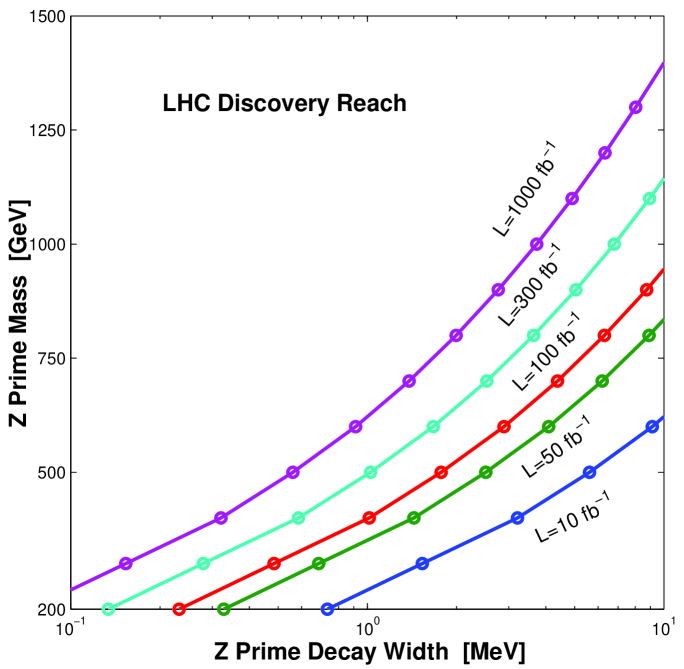
Figure 9: A plot of the discovery reach of the LHC for small StSM $Z^{\prime}$ widths. The allowed regions are to the right and below each curve for a given luminosity. This figure is a blown up version of the very low $Z^{\prime}$ width region of Fig (8).

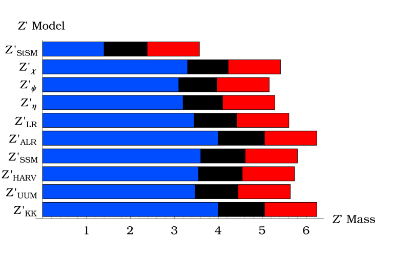
Figure 10: The discovery reach for $Z^{\prime}$ in StSM (without detector cuts) and several other $Z^{\prime}$ models at the LHC. The length of the bars indicate integrated luminosities of 10 ${\rm{fb}}^{-1}$ (blue), 100 ${\rm{fb}}^{-1}$ (black), and 1000 ${\rm{fb}}^{-1}$ (red) using 10 events as the criterion for discovery [43, 44]. The analysis indicates that the $Z^{\prime}$ of StSM can be probed up to $\approx$ 3.5 TeV at the LHC with 1000 ${\rm{fb}}^{-1}$ of integrated luminosity. With inclusion of detector cuts the discovery reach of the LHC for the StSM $Z^{\prime}$ comes down to about 3 TeV.

In Fig. (8) we give the discovery reach for finding the StSM $Z^{\prime}$ with various values of $\epsilon$ as a function of $M_{Z^{\prime}}$ for integrated luminosities in the range 10 ${\rm{fb}}^{-1}$ to 1000 ${\rm{fb}}^{-1}$. The criterion used for the discovery limit in the analysis given here is an assumption that $5\sqrt{N_{SM}}$ events or 10 events, whichever is larger, constitutes a signal where $N_{SM}$ is the SM background, and we have scaled the bin size with $M_{Z^{\prime}}$ appropriate for the ATLAS detector with a conservative lower limit of 20 GeV below .5 TeV. In this part of the analysis we have assumed that detector effects can lead to signal and background losses of 50 percent (see Section (8.2)). If better efficiency and acceptance cuts are available, the discovery reach of the LHC for finding a $Z^{\prime}$ will be even higher than what we have displayed. With an assumption of efficiencies as stated above, one finds that with 100 ${\rm{fb}}^{-1}$ of integrated luminosity, one can explore a $Z^{\prime}$ up to about 2 TeV with $\epsilon=0.06$, and this limit can be pushed to $\approx$ 3 TeV with 1000 ${\rm{fb}}^{-1}$ of integrated luminosity. Further, one finds that for 1000 ${\rm{fb}}^{-1}$ of integrated luminosity, one can explore a $Z^{\prime}$ up to about 2 TeV for $\epsilon$ as low as $\lesssim 0.02$. Also displayed in Fig. (8) are the discovery limits for different decay widths as a function of the $Z^{\prime}$ mass again for luminosities in the range 10 ${\rm{fb}}^{-1}$ and 1000 ${\rm{fb}}^{-1}$. Here one finds that the LHC can probe a 100 MeV $Z^{\prime}$ up to about 2.75 TeV and a 10 MeV width up to a $Z^{\prime}$ mass of about 1.5 TeV. A more detailed exhibition of the capability of the LHC to probe the StSM $Z^{\prime}$ model is given in Fig. (9). Here one finds that the StSM model with a $Z^{\prime}$ width even in the MeV and sub-MeV range will produce a detectable signal in the dilepton channel in the Drell-Yan process with luminosities accessible at the LHC. While the analysis above is for the specific StSM model, the general features of this analysis may hold for a wider class of models which support narrow resonances. In Fig. (10) we give a comparison of the LHC’s ability to probe the narrow StSM $Z^{\prime}$ relative to other $Z^{\prime}$ models [43, 44] to address the question of how the StSM $Z^{\prime}$ “stacks up” to these models. In order to make the appropriate comparisons of the discovery limits for the StSM with the other $Z$ prime models we do not impose detector cuts on the StSM $Z^{\prime}$ limits displayed in Fig. (10), since such cuts were not imposed for the discovery limits of other $Z^{\prime}$ models shown in Fig. (10). The analysis of Fig. (10) shows that the StSM $Z^{\prime}$, even with its exceptionally narrow width, may be probed on scales comparable with models that have resonance widths of the order of several GeV or higher.

8 Comparison of Stueckelberg $Z^{\prime}$ with a Massive Graviton of Warped Geometry at the LHC

As discussed above one finds that the Stueckelberg $Z^{\prime}$ boson is a very narrow resonance which sets it apart from all other $Z^{\prime}$ models. However, there is another class of models, i.e., models based on warped geometry [9, 10] (labeled RS models), which can mimic the Stueckelberg $Z^{\prime}$ in a certain part of the parameter space as far as the narrowness of the resonance is concerned. It was shown in the analysis of Ref. [4] that the signature spaces for these two models lie close to each other in certain regions of their respective parameter spaces, but the models are still distinguishable in the dilepton mass region accessible at the Tevatron. Here we extend the analysis of their relative signatures to the LHC energies. The geometry of RS models is a slice of $AdS_{5}$ described by the metric $ds^{2}$ =$exp(-2kr_{c}|\phi|)\eta_{\mu\nu}dx^{\mu}dx^{\nu}-r_{c}^{2}d\phi^{2}$, $0\leq\phi\leq\pi$, where $r_{c}$ is the radius of the extra dimension and $k$ is the curvature of $AdS_{5}$, which is taken to be the order of the Planck scale. We work in the regime where the SM particles are confined to the TeV scale brane, while gravity is propagating in the bulk [9, 45]. The effective scale that enters in the electroweak region is the scale $\Lambda_{\pi}=\bar{M}_{Pl}exp(-kr_{c}\pi)$, and for reasons of naturalness it is typically constrained by the condition $\Lambda_{\pi}<10$ TeV. Values of $k/{\bar{M}_{Pl}}$ over a wide range $10^{-5}-.1$ have been considered in the literature [47]. However, the range below $.01$ appears to be eliminated from the electroweak constraints. In this analysis we consider the lightest massive graviton mode .

8.1 Drell-Yan Cross Sections via a Massive Graviton of Warped Geometry

We consider the process $pp\to G\to f\bar{f}$ for the first massive graviton mode in the RS model. The partonic production cross section for this mode receives contributions both from quarks and gluons, and is given by [49, 50, 52, 54, 55]

$$\frac{{d\sigma_{q\bar{q}}^{G}}}{{dz}}+\frac{{d\sigma_{gg}^{G}}}{{dz}}=\frac{1}{2}\frac{{\kappa^{4}M^{6}}}{{320\pi^{2}}}\left[{\Delta_{q\bar{q}}(z)+\Delta_{gg}(z)}\right]\frac{1}{{(M^{2}-M_{G}^{2})^{2}+M^{2}\Gamma_{G}^{2}}}.$$ (66)

The total decay width that enters above is given by the sum of the partial widths which are [49, 51, 52]

$$\Gamma(G\to V\bar{V})=\delta\frac{\kappa^{2}M^{3}_{G}}{80\pi}(1-4{\delta}_{V})^{1/2}\left(\frac{13}{12}+\frac{14}{3}{\delta}_{V}+4{\delta}^{2}_{V}\right)\theta(M_{G}-2M_{V})$$ (67)

$$\Gamma(G\to f\bar{f})=N^{c}_{f}\frac{\kappa^{2}M^{3}_{G}}{320\pi}(1-4{\delta}_{f})^{3/2}(1+\frac{8}{3}{\delta}_{f})\theta(M_{G}-2m_{f})$$ (68)

$$\Gamma(G\to gg)=\frac{\kappa^{2}M^{3}_{G}}{20\pi}$$ (69)

$$\Gamma(G\to\gamma\gamma)=\frac{\kappa^{2}M^{3}_{G}}{160\pi}.$$ (70)

Here $\delta_{f}=m^{2}_{f}/M^{2}_{G}$, $\delta_{V}=M^{2}_{V}/M^{2}_{G}$, and $\delta=(1/2,1)$ for $(V=W,Z)$. For the first massive mode, $\kappa$ is given by [51, 52, 54]

$$\kappa=\sqrt{2}\frac{{x_{1}}}{{m_{G}}}\frac{k}{{\bar{M}_{Pl}}}$$ (71)

where $x_{1}=3.8317$ is the first root of the Bessel function of order 1, and $\bar{M}_{Pl}$ is the reduced Planck mass in four dimensions ($\bar{M}_{Pl}=M_{Pl}/\sqrt{8\pi}$). The leading order angular dependance is given in terms of [52, 54, 55]

$$\Delta_{q\bar{q}}(z)=\frac{\pi}{{8N_{c}}}\frac{5}{8}(1-3z^{2}+4z^{4}),\hskip 28.45274pt\Delta_{gg}(z)=\frac{\pi}{{2(N_{c}^{2}-1)}}\frac{5}{8}(1-z^{4}).$$ (72)

In the narrow width approximation we have to NLO

$$\frac{d\sigma^{G}_{pp}}{dz} = K^{G}(M_{G}^{2})\frac{1}{{2s}}\frac{{\kappa^{4}M_{G}^{6}}}{{320\pi^{2}}}\frac{\pi}{{M_{G}\Gamma_{G}}}\times$$

$$\hskip 14.22636pt\left[{\sum\limits_{q}{\Delta_{q\bar{q}}(z)}{\mathcal{W}}_{\left\{{pp(q\bar{q})}\right\}}(s,M_{G}^{2})+{\Delta_{gg}(z)}{\mathcal{W}}_{\left\{{pp(gg)}\right\}}(s,M_{G}^{2})}\right]$$

where ${\mathcal{W}}_{pp(q\bar{q})}$ is defined in Section 6 and ${\mathcal{W}}_{pp(gg)}$ is defined by

$$\mathcal{W}_{\left\{{pp}\left(gg\right)\right\}}(\tau)=\int_{0}^{1}\int_{0}^{1}dxdy\delta(\tau-xy)f_{g,p}(x)f_{g,p}(y),$$ (74)

and the more strongly mass dependant RS $K$ factor ($K^{G}$) is discussed in detail in Refs. [55]. The production cross section including the quark and gluon contributions is in the narrow width approximation given by

$$\hskip 14.22636pt\sigma\cdot Br(G\to l^{+}l^{-})=K^{G}(M_{G}^{2})\frac{1}{s}\frac{{\kappa^{4}M_{G}^{6}}}{{{\rm{15360}}}}\frac{1}{{M_{G}\Gamma_{G}}}\sum\limits_{q}{{\mathcal{W}}_{\left\{{pp(q\bar{q})}\right\}}}(s,M_{G}^{2})$$ (75)

$$\hskip 113.81102pt+K^{G}(M_{G}^{2})\frac{1}{s}\frac{{\kappa^{4}M_{G}^{6}}}{{{\rm{10240}}}}\frac{1}{{M_{G}\Gamma_{G}}}{\mathcal{W}}_{\left\{{pp(gg)}\right\}}(s,M_{G}^{2}).$$

8.2 Signature Spaces of StSM $Z^{\prime}$ and of the Warped Geometry Graviton

A relative comparison of the StSM and of the RS model is given in Table (3) where the decay width of the Stueckelberg $Z^{\prime}$ boson for the case $\epsilon=0.06$ is given as a function of the $Z^{\prime}$ mass in the range (1000-3000) GeV, and the corresponding $\sigma\cdot Br(G\to l^{+}l^{-})$ is exhibited. Also shown are the decay widths for an RS graviton in the same mass range for $k/{\bar{M}_{Pl}}=0.01$.

Quite remarkably, the spin 1 $Z^{\prime}$ of the StSM and the spin 2 massive graviton of the RS model have nearly identical signatures in terms of the decay widths and the production cross sections around a resonance mass of 2 TeV (with or without out detector cuts). In Table (4) we give an analysis of the number of events that can be observed in the ATLAS detector with 100 ${\rm{fb}}^{-1}$ of integrated luminosity. One finds that for high masses the number of events that one expects to see at the LHC for the StSM $Z^{\prime}$, with $\epsilon=0.06$, are similar to the number of events one expects for the RS model for $k/\bar{M}_{Pl}=0.01$. For the case of the RS model, simulations conducted by Ref. [51] show that overall detector losses range from (27-38) percent between (500-2200) GeV, and we have extrapolated these cuts to the 3 TeV mass region. For the case of $Z^{\prime}$, which has a different angular dependancy than the graviton due to spin, we have assumed a uniform 50 percent loss of events at in the range of $Z^{\prime}$ mass investigated. This reduction factor is consistent with the reduction factor used by Ref. [58], and is similar to the reduction factor used by other groups [59]. For the SM background, denoted as $N_{B}=N_{SM}$, the same detector loss is assumed, and it can be seen in Table (4) that this simulation is in good agreement with the analysis of Ref. [51]. Of course a slightly more realistic analysis of the number of events that may be observed requires simulating detector efficiencies more accurately, which in turn requires the implementation of the StSM couplings in event generation simulators [60, 61, 62, 63, 58].

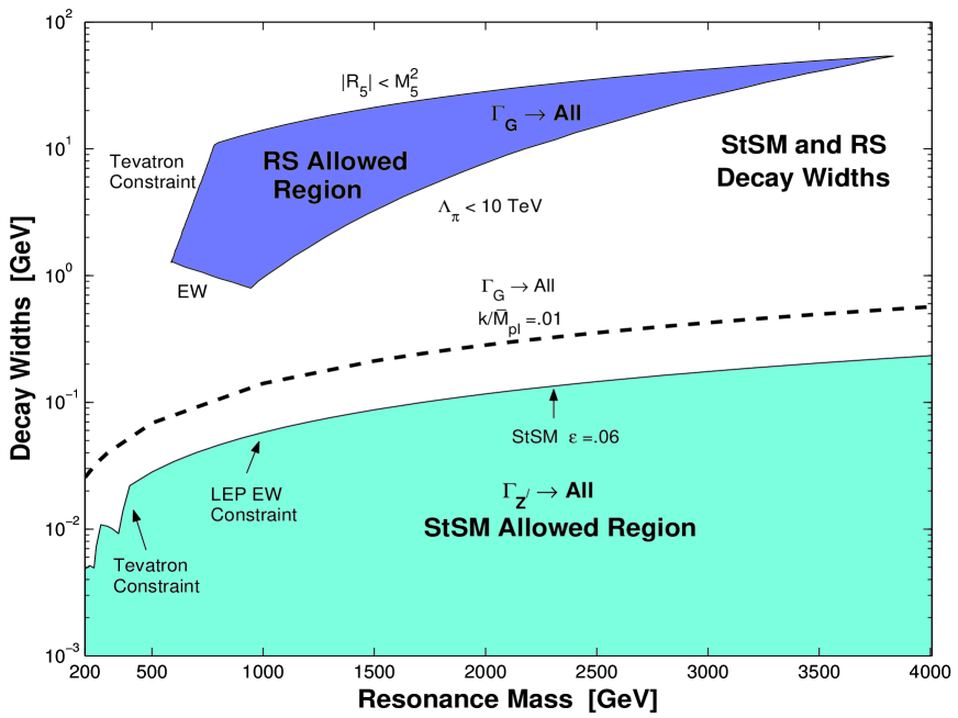
Figure 11: A comparison of the allowed region in resonance decay width - resonance mass plane for the $Z^{\prime}$ in the StSM and the first graviton mode in the RS model. The dashed line is for the RS case with $k/{\bar{M}}_{Pl}=.01$. The allowed (shaded) regions are constructed by utilizing the constrained parameter spaces of StSM [4] and the RS model [45, 46, 37].

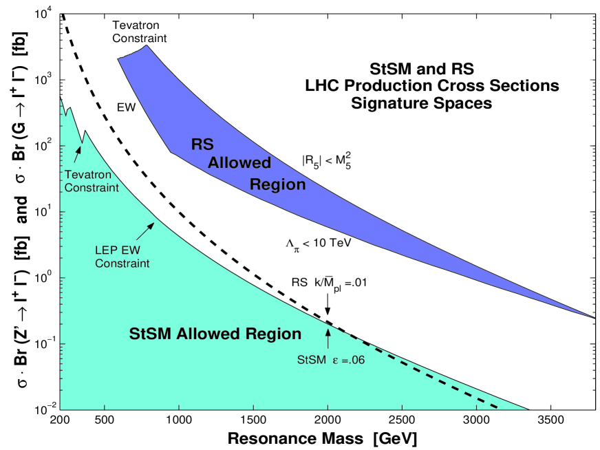
Figure 12: A comparison of the LHC signature spaces in the dilepton channel using $\sigma(pp\to Z^{\prime}\to l^{+}l^{-})$ for the $Z^{\prime}$ production and its decay into dileptons for the StSM and using $\sigma(pp\to G\to l^{+}l^{-})$ for the production of the graviton and its decay into dileptons for the RS model. The dashed line is for the RS case with $k/{\bar{M}}_{Pl}=.01$. The allowed regions are constructed by utilizing the constrained parameter spaces of StSM [4] and of the RS model [45, 46, 37].

In Fig. (11) we give a comparison of the signature spaces for the decay of the StSM $Z^{\prime}$ and of the RS graviton in the warped geometry model using the decay width-resonance mass plane. The allowed regions (shaded) for the two models are exhibited, where the unshaded regions correspond to constrained regions of the parameter spaces of the two models. One finds that although there is a region of the parameter space of the RS model where the decay widths can be narrow, the region of potential overlap with the StSM is avoided if one includes the constrains of the oblique parameters [64, 65]. Fig. (12) gives a more direct method for differentiating the two classes of models. Here one has plots of $\sigma\cdot Br(Z^{\prime}\to l^{+}l^{-})$ and $\sigma\cdot Br(G\to l^{+}l^{-})$ as a function of the resonance mass. One finds that the allowed regions of the signature space of the two models consistent with the parameter space constraints provides a clear differentiation between these two classes of models. Thus Fig. (12) provides an important tool for establishing the nature of the resonance once a narrow resonance is discovered. Thus, for example, the $\sigma\cdot Br(Z^{\prime}\to l^{+}l^{-})$ is an order of magnitude or more smaller than $\sigma\cdot Br(G\to l^{+}l^{-})$ over most of the dilepton invariant mass that will be probed by the Drell-Yan process at the LHC.

8.3 Angular Distributions in the Dilepton Channel in $pp\to(Z^{\prime},G)\to l^{+}l^{-}$

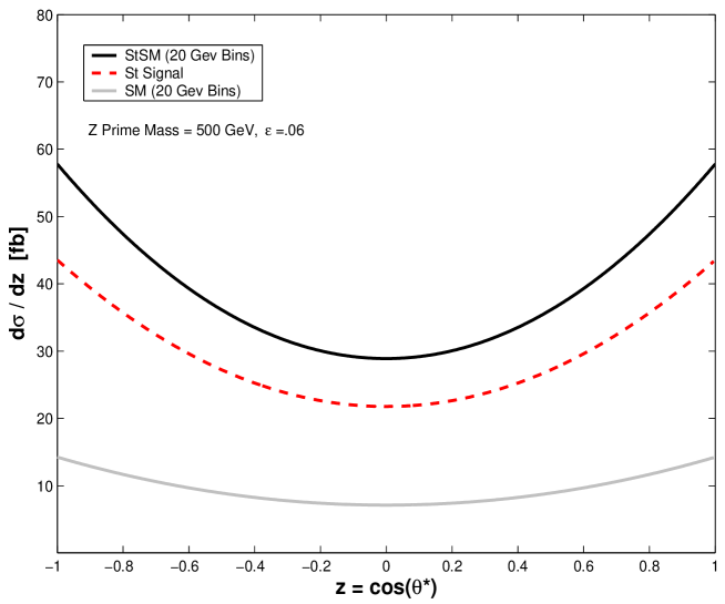
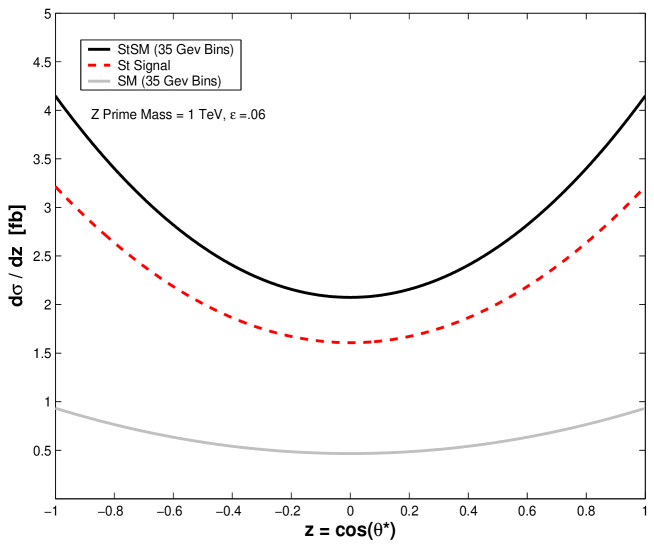
Figure 13: Angular distribution $d\sigma/dz$ vs $z=\cos(\theta^{*})$ in the dilepton center of mass frame in the decay $Z^{\prime}\to l^{+}l^{-}$ in StSM for $Z^{\prime}$ mass of 500 GeV (upper graph) and 1 TeV (lower graph). The SM background is also shown, and the StSM contribution sits high above it.

Angular distributions in the C-M frame of the final dilepton state give clear signatures of the spin of the produced particle in the Drell-Yan process (for recent works see, for example, Refs.[53, 66]). Thus angular distributions are a powerful tool in distinguishing the StSM $Z^{\prime}$, a spin 1 particle, from the massive graviton of warped geometry, a spin 2 particle. The CDF group has already carried out angular distribution analyses [39] using the cumulative data at the Tevatron and more detailed analyses are likely to follow. Similar analyses at the LHC would allow one to investigate the spin of an observed resonance with much more data. In the following we give a relative comparison of the angular distributions arising from the StSM $Z^{\prime}$ and from the massive gravtion of warped geometry. To this end we first examine the feasibility of distinguishing the StSM $Z^{\prime}$ signal from the Standard Model background. This is done in Fig. (13) for $Z^{\prime}$ masses of 500 GeV and as well as 1 TeV with a bin size of 20 GeV and 35 GeV respectively. Fig. (13) shows that the StSM $Z^{\prime}$ signal in this case is distinct from the $\gamma,Z$ background. Second, the StSM angular distribution sits high above the SM background and thus an observation of such a distribution can lead to an identification of new physics in the dilepton channel.

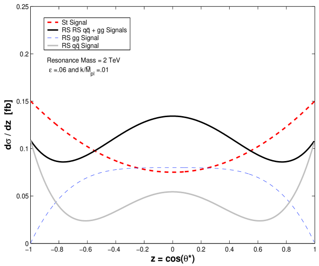
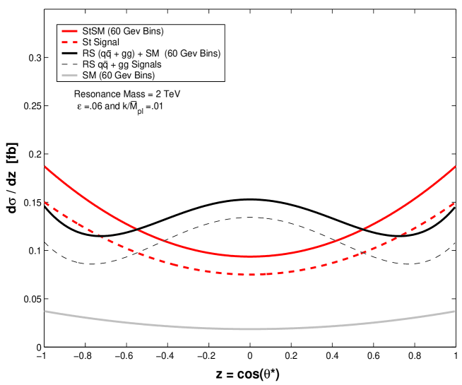
Figure 14: An exhibition of the angular distribution $d\sigma(pp\to Z^{\prime}\to l^{+}l^{-})/dz$ for the StSM model and $d\sigma(pp\to G\to l^{+}l^{-})/dz$ for the RS model in the dilepton center of mass system, as defined in Eqs. (61,8.1). For the StSM, $\epsilon$ is taken at .06 and $G$ is the first resonant mode of the RS model, with $(k/\bar{M}_{Pl})=.01$ and the resonance mass is 2 TeV in each case. For the RS model the parameter choice requires relaxing the oblique constraints and the constraint on $\Lambda_{\pi}$.

Next we give a relative comparison of the angular distribution in the dilepton channel arising from the StSM $Z^{\prime}$ and the massive graviton of warped geometry. This is done in Fig. (14) for a resonance mass of 2 TeV, the mass region where an overlap between the two models can occur if the constraints on the RS model are relaxed. The top graph in Fig. (14) gives the angular distributions arising for the $Z^{\prime}$ exchange but without the Standard Model background, i.e., what is plotted is the pure signal. Also plotted is the pure signal from the graviton exchange which consists of contributions from the quarks and the gluons which are separately exhibited. In the lower graph of Fig. (14) the angular distributions arising for the StSM $Z^{\prime}$ and for the massive graviton exchanges including the Standard Model background are exhibited. The graph shows that the signal plus the background lies significantly higher than the SM background, and further the sum of the $Z^{\prime}$ signal and the SM background is easily distinguishable from the sum of the massive graviton signal and the SM background. The angular distributions for the graviton exchange are sensitively dependent on the graviton mass, mainly due to the sensitivity of the PDF [33] for the gluon on the mass scale. Thus the angular distributions for the graviton will change with the mass scale and change significantly. However, the angular distributions for the $Z^{\prime}$ and for the graviton will continue to be identifiably distinct and allow one to distinguish between these two classes of narrow resonance models.

9 Conclusions

In this paper we have carried out an investigation of narrow resonances with specific focus on two classes of models which have recently emerged where narrow resonances arise quite naturally. The first of these are the Higgless extensions of the Standard Model gauge group, and of the Left-Right symmetric model gauge group where the extra gauge boson becomes massive via the Stueckelberg mechanism. A narrow $Z^{\prime}$ naturally arises in these models. The second class of models are those based on warped geometry which give rise to a narrow graviton resonance for $k/\bar{M}_{Pl}\sim.01$. The main focus of this paper was to investigate the capability of the LHC to discover narrow resonances specifically belonging to these classes of models and to discriminate between them by examining their signature spaces. For the Stueckelberg model we discussed the constraints on the parameters space of the model using the LEP data and the CDF and DØ data. These constraints were then utilized to explore the narrow Stueckelberg $Z^{\prime}$ at the LHC. The analysis using the dilepton production in the Drell-Yan process via the $Z^{\prime}$ boson shows that one will be able to explore a narrow $Z^{\prime}$ resonance of Stueckelberg origin up to about 2 TeV with 100 ${\rm{fb}}^{-1}$ of integrated luminosity and further up to 2.5 TeV with 300 ${\rm{fb}}^{-1}$ of integrated luminosity. With 1000 ${\rm{fb}}^{-1}$ of integrated luminosity one could even explore a Stueckelberg $Z^{\prime}$ beyond 3 TeV. The results of this analysis are summarized in Fig. (8) and Fig. (10).

We carried out a similar analysis for the dilepton production in the warped geometry RS model which also has the potential of supporting a narrow resonance. It is then interesting to ask how a Stueckelberg type narrow resonance could be distinguished from a narrow massive graviton of warped geometry. Indeed there is a range of the parameter space where an overlap exists between the two models with the width of the massive graviton of the warped geometry being similar to the width of the $Z^{\prime}$ arising from the Stueckelberg model. We have shown that one of the clear distinguishing features between them is $\sigma\cdot Br(l^{+}l^{-})$ for dilepton production in the Drell-Yan process which proceeds through the interaction $pp\to Z^{\prime}\to l^{+}l^{-}$ for the Stueckelberg model and via $pp\to G\to l^{+}l^{-}$ for the case of the RS model. The analysis of Fig. (12) shows that for any resonance mass the signature spaces of the StSM and of the RS model are distinct and one can discriminate between them using the $\sigma\cdot Br(l^{+}l^{-})$ criterion. In addition, the angular distributions in the dilepton center of mass system provide a clear discrimination between the two models. Here one finds that the angular distributions from the StSM $Z^{\prime}$ and from the massive graviton lie well above the Standard Model background and further are distinctly dissimilar as exhibited in the analysis of Fig. (14).

Some general features of the searches for narrow resonances were also discussed. The bin size used in data collection has a direct bearing on the signal to background ratio as shown in Fig. (7). The analysis presented in this paper reveals the remarkable phenomenon that the models considered here can be tested even when the resonance widths are small and the resonance masses are large. Specifically one finds that the StSM model can produce observable cross section signals with a $Z^{\prime}$ width lying in the MeV or even in the sub-MeV range while the $Z^{\prime}$ mass may be in hundreds of GeV to TeV range. This phenomenon is exhibited in Fig. (9). While the result of Fig. (9) is presented for the specific case of StSM $Z^{\prime}$ model, similar considerations may apply to a wider class of models which support a narrow resonance. The evidence for a narrow resonance will be an important hint for an altogether new type of physics beyond the Standard Model and possibly a hint of a string origin.

Quantity	Value (Exp.)	StSM	$\Delta$Pull
$\Gamma_{Z}$ [GeV]	2.4952 $\pm$ 0.0023	(2.4952-2.4942)	(0.2, 0.6)
$\sigma_{had}$ [nb]	41.541 $\pm$ 0.037	(41.547-41.568)	(-0.3, -0.9)
$R_{e}$	20.804 $\pm$ 0.050	(20.753-20.761)	(-0.1, -0.2)
$R_{\mu}$	20.785 $\pm$ 0.033	(20.800-20.761)	(-0.1, -0.4)
$R_{\tau}$	20.764 $\pm$ 0.045	(20.791-20.807)	(-0.1, -0.3)
$R_{b}$	0.21643 $\pm$ 0.00072	(0.21575-0.21573)	(0.0, 0.0)
$R_{c}$	0.1686 $\pm$ 0.0047	(0.1711-0.1712)	(0.0, 0.0)
$A^{(0,e)}_{FB}$	0.0145 $\pm$ 0.0025	(0.0168-0.0175)	(-0.2, -0.5)
$A^{(0,\mu)}_{FB}$	0.0169 $\pm$ 0.0013	(0.0168-0.0175)	(-0.3, -0.9)
$A^{(0,\tau)}_{FB}$	0.0188 $\pm$ 0.0017	(0.0168-0.0175)	(-0.2, -0.7)
$A^{(0,b)}_{FB}$	0.0991 $\pm$ 0.0016	(0.1045-0.1070)	(-0.8, -2.3)
$A^{(0,c)}_{FB}$	0.0708 $\pm$ 0.0035	(0.0748-0.0766)	(-0.3, -0.8)
$A^{(0,s)}_{FB}$	0.098 $\pm$ 0.011	0.105-0.107)	(-0.1, -0.3)
$A_{e}$	0.1515 $\pm$ 0.0019	(0.1491-0.1524)	(-1.0, -2.8)
$A_{\mu}$	0.142 $\pm$ 0.015	(0.149-0.152)	(-0.1, -0.4)
$A_{\tau}$	0.143 $\pm$ 0.004	(0.149-0.152)	(-0.5, -1.3)
$A_{b}$	0.923 $\pm$ 0.020	(0.935-0.935)	(0.0, 0.0)
$A_{c}$	0.671 $\pm$ 0.027	(0.669-0.670)	(0.0, 0.1)
$A_{s}$	0.895 $\pm$ 0.091	(0.936-0.936)	(0.0, 0.0)

Table 1: Results of the StSM fit to a standard set of electroweak observables at the $Z$ pole for $\epsilon$ in the range $(.035-.059)$ for $M_{1}=350$ GeV. The Pulls are calculated as shifts from the SM fit via $\Delta{\rm Pull}=({\rm SM-StSM})/\delta{\rm Exp}$ and Pull(StSM)=Pull(SM)+ $\Delta$Pull. The data in column 2 is taken from Ref. [67].

Quantity	StSM	StLR
$\epsilon=M_{2}/M_{1}$	.060	.071
$M_{Z^{\prime}}$ [GeV]	500	500
($v^{\prime}_{\nu}$ , $a^{\prime}_{\nu}$)	(0.014638, 0.014638)	(0.014615, 0.014621)
($v^{\prime}_{e}$ , $a^{\prime}_{e}$)	(0.042401, -0.014638)	(0.042352, -0.014621)
($v^{\prime}_{u}$ , $a^{\prime}_{u}$)	(-0.023388, 0.014638)	(-0.023363, 0.014621)
($v^{\prime}_{d}$ , $a^{\prime}_{d}$ )	(0.004375, -0.014638)	(0.004374, -0.014621)
$\Gamma_{Z}$ [GeV]	0.0297	0.0299
$Br(\nu_{e}\bar{\nu}_{e})$	2.36%	2.60%
$Br(e^{+}e^{-})$	12.33%	12.33%
$Br(u\bar{u})$	14.52%	14.42%
$Br(d\bar{d})$	4.45%	4.42%
$Br(t\bar{t})$	10.93%	10.85%
$Br(W^{+}W^{-})$	2.60%	2.56%

Table 2: Comparison of the $Z^{\prime}$ branching ratios in StSM and StLR model at $M_{Z^{\prime}}=500$ GeV for the maximum allowed value of $\epsilon$ consistent with the analysis of Sec. (4.1). The couplings and branching ratios for the $Z^{\prime}$ in the two models turn out be remarkably close.

$(M_{Z^{\prime}},M_{G})$	$\Gamma_{Z^{\prime}}$ (GeV)	$\Gamma_{G}$ (GeV)	$\sigma_{Z^{\prime}}\cdot Br$ (fb)	$\sigma_{G}\cdot Br$ (fb)
1000	0.058	0.141	4.29	9.98
1250	0.073	0.176	1.72	3.11
1500	0.087	0.212	0.779	1.15
1750	0.102	0.247	0.384	0.475
2000	0.117	0.283	0.200	0.215
2250	0.131	0.318	0.109	0.104
2500	0.146	0.354	0.061	0.053
2750	0.160	0.389	0.035	0.028
3000	0.175	0.425	0.021	0.015

Table 3: A comparison of the narrow resonance widths and $\sigma.Br(l^{+}l^{-})$ in StSM for $\epsilon=.06$ and in the RS warped geometry with $k/{\bar{M}}_{Pl}=.01$ as a function of the resonance mass in GeV.

$(M_{Z^{\prime}},M_{G})$	Bin (GeV)	$N_{SM}$	$N_{S}=(N_{St},N_{RS})$	$N^{min}_{S}$
1000	30.65	54.45	(214.33,716.96)	36.90
1250	36.79	20.95	(85.90,216.96)	22.89
1500	42.89	9.22	(38.94,77.73)	15.18
1750	48.96	4.44	(19.18,31.30)	10.53
2000	55.02	2.27	(10.01,13.72)	10
2250	61.07	1.22	(5.46,6.41)	10
2500	67.11	0.68	(3.07,3.15)	10
2750	73.14	0.39	(1.77,1.60)	10
3000	79.17	0.22	(1.04,0.84)	10

Table 4: A comparison of the signal events with integrated luminosity of $\mathcal{L}=$ 100 $\rm fb^{-1}$ in the StSM for the case $\epsilon=.06$ with the signal in the RS warped geometry for $k/{\bar{M}}_{Pl}=.01$ including ATLAS detector effects as a function of the resonance mass in GeV. Acceptance($A$) and efficiency($\varepsilon$) for the RS case is as in Ref. [51], while for the StSM we use the spin 1 detector losses given in Ref. [58] $\approx$ 50 % as discussed in the text. For $X=(Z^{\prime},G)$ of Table 3, $N_{S}=(\sigma\cdot Br)\varepsilon A\mathcal{L}$, $N_{B}=N_{SM}$ (background integrated over the bin), $N_{S}^{min}=5\sqrt{N_{B}}$ or 10, whichever is larger. The minimum signal cross section is $(\sigma\cdot Br)^{\mathrm{min}}=(\varepsilon A\mathcal{L})^{-1}N_{S}^{min}$ for each model.

References

- [1] B. Kors and P. Nath, “A Stueckelberg extension of the standard model,” Phys. Lett. B 586, 366 (2004); [arXiv:hep-ph/0402047];
- [2] B. Kors and P. Nath, “A supersymmetric Stueckelberg U(1) extension of the MSSM,” JHEP 0412, 005 (2004); [arXiv:hep-ph/0406167];
- [3] B. Kors and P. Nath, “Aspects of the Stueckelberg extension,” JHEP 0507, 069 (2005). [arXiv:hep-ph/0503208].
- [4] D. Feldman, Z. Liu and P. Nath, Probing a very narrow Z’ boson with CDF and DØ data, [arXiv:hep-ph/0603039] (Accepted for publication in Phys. Rev. Lett.).
- [5] I. Antoniadis, E. Kiritsis and T. N. Tomaras, Phys. Lett. B 486, 186 (2000) [arXiv:hep-ph/0004214]; L. E. Ibanez, F. Marchesano and R. Rabadan, JHEP 0111 (2001) 002; R. Blumenhagen, V. Braun, B. Körs and D. Lüst, hep-th/0210083; I. Antoniadis, E. Kiritsis, J. Rizos and T. N. Tomaras, Nucl. Phys. B 660, 81 (2003);
- [6] D. M. Ghilencea, L. E. Ibanez, N. Irges and F. Quevedo, TeV-scale Z′ Bosons from D-branes, JHEP 0208 (2002) 016, D. M. Ghilencea, U(1) Masses in Intersecting D-brane SM-like Models, Nucl. Phys. B 648 (2003) 215.
- [7] C. Coriano’, N. Irges and E. Kiritsis, Nucl. Phys. B 746, 77 (2006) [arXiv:hep-ph/0510332]; P. Anastasopoulos, T. P. T. Dijkstra, E. Kiritsis and A. N. Schellekens, arXiv:hep-th/0605226; P. Anastasopoulos, M. Bianchi, E. Dudas and E. Kiritsis, arXiv:hep-th/0605225.
- [8] B. Kors and P. Nath, “How Stueckelberg extends the standard model and the MSSM,” arXiv:hep-ph/0411406., published in Boston 2004, Particles, strings and cosmology, edited by G. Alverson et.al., World Scientific. p. 437-447
- [9] L. Randall and R. Sundrum, Phys. Rev. Lett. 83, 3370 (1999).
- [10] M. Gogberashvili, Int. J. Mod. Phys. D 11, 1635 (2002) [arXiv:hep-ph/9812296].
- [11] D. London and J. L. Rosner, Phys. Rev. D 34, 1530 (1986).
- [12] J. L. Hewett and T. G. Rizzo, Phys. Rept. 183, 193 (1989).
- [13] M. Cvetic and P. Langacker, Phys. Rev. D 54, 3570 (1996).
- [14] K. S. Babu, C. F. Kolda and J. March-Russell, Phys. Rev. D 57, 6788 (1998) [arXiv:hep-ph/9710441].
- [15] G. C. Cho, K. Hagiwara and Y. Umeda, Nucl. Phys. B 531, 65 (1998) [Erratum-ibid. B 555, 651 (1999)] [arXiv:hep-ph/9805448].
- [16] A. Leike, Phys. Rept. 317, 143 (1999).
- [17] C. T. Hill and E. H. Simmons, Phys. Rept. 381, 235 (2003) [Erratum-ibid. 390, 553 (2004)] [arXiv:hep-ph/0203079].
- [18] M. Carena, A. Daleo, B. A. Dobrescu and T. M. P. Tait, Phys. Rev. D 70, 093009 (2004).
- [19] V. Barger, P. Langacker, H. S. Lee and G. Shaughnessy, arXiv:hep-ph/0603247.
- [20] V. D. Barger and K. Whisnant, Phys. Rev. D 36, 3429 (1987).
- [21] B. Dutta and S. Nandi, Phys. Lett. B 315, 134 (1993).
- [22] R. N. Mohapatra and J. C. Pati, Phys. Rev. D 11, 2558 (1975); R. N. Mohapatra and G. Senjanovic, Phys. Rev. Lett. 44, 912 (1980).
- [23] R. Arnowitt and P. Nath, Phys. Rev. D 46, 3981 (1992); T. Ibrahim and P. Nath, Phys. Rev. D 63, 035009 (2001) [arXiv:hep-ph/0008237].
- [24] P. Nath and M. Yamaguchi, Phys. Rev. D 60, 116004 (1999); M. Masip and A. Pomarol, Phys. Rev. D 60, 096005 (1999);R. Casalbuoni, S. De Curtis, D. Dominici and R. Gatto, Phys. Lett. B 462, 48 (1999);T. G. Rizzo and J. D. Wells, Phys. Rev. D 61, 016007 (2000); C. D. Carone, Phys. Rev. D 61, 015008 (2000).
- [25] W. J. Marciano, Phys. Rev. D 60, 093006 (1999).
- [26] W. J. Marciano and A. Sirlin, Phys. Rev. D 29, 945 (1984).
- [27] [ALEPH Collaboration], [arXiv:hep-ex/0509008].
- [28] U. Baur, O. Brein, W. Hollik, C. Schappacher and D. Wackeroth, Phys. Rev. D 65, 033007 (2002).
- [29] D. Y. Bardin,M. Grunewald and G. Passarino, [arXiv:hep-ph/9902452].
- [30] J. Erler and P. Langacker, [arXiv:hep-ph/0407097].
- [31] J. Kang and P. Langacker, Phys. Rev. D 71, 035014 (2005) [arXiv:hep-ph/0412190].
- [32] R. Hamberg, W. L. van Neerven and T. Matsuura,’ Nucl. Phys. B 359, 343 (1991).
- [33] J. Pumplin, D. R. Stump, J. Huston, H. L. Lai, P. Nadolsky and W. K. Tung, JHEP 0207, 012 (2002).
- [34] M. C. Kumar, P. Mathews and V. Ravindran, arXiv:hep-ph/0604135.
- [35] N. Arkani-Hamed, G. L. Kane, J. Thaler and L. T. Wang, arXiv:hep-ph/0512190.
- [36] Information is available at http://www-cdf.fnal.gov/harper/diEleAna.html .
- [37] V. M. Abazov et al. [DØ Collaboration], Phys. Rev. Lett. 95, 091801 (2005) [arXiv:hep-ex/0505018].
- [38] A. Abulencia et al. [CDF Collaboration], Phys. Rev. Lett. 95, 252001 (2005) [arXiv:hep-ex/0507104].
- [39] A. Abulencia et al. [CDF Collaboration], Phys. Rev. Lett. 96, 211801 (2006) [arXiv:hep-ex/0602045].
- [40] I. Antoniadis, K. Benakli and M. Quiros, Phys. Lett. B 460, 176 (1999) [arXiv:hep-ph/9905311].
- [41] P. Nath, Y. Yamada and M. Yamaguchi, Phys. Lett. B 466, 100 (1999) [arXiv:hep-ph/9905415].
- [42] M. Dittmar, A. S. Nicollerat and A. Djouadi, Phys. Lett. B 583, 111 (2004) [arXiv:hep-ph/0307020].
- [43] S. Godfrey, in Proc. of the APS/DPF/DPB Summer Study on the Future of Particle Physics (Snowmass 2001) ed. N. Graf, eConf C010630, P344 (2001) [arXiv:hep-ph/0201093].
- [44] M. Cvetic and S. Godfrey, arXiv:hep-ph/9504216.
- [45] H. Davoudiasl, J. L. Hewett and T. G. Rizzo, Phys. Rev. Lett. 84, 2080 (2000).
- [46] H. Davoudiasl, J. L. Hewett and T. G. Rizzo, Phys. Rev. D 63, 075004 (2001) [arXiv:hep-ph/0006041].
- [47] A. V. Kisselev, Phys. Rev. D 73, 024007 (2006) [arXiv:hep-th/0507145].
- [48] G. Weiglein et al. [LHC/LC Study Group], arXiv:hep-ph/0410364.
- [49] T. Han, J. D. Lykken and R. J. Zhang, Phys. Rev. D 59, 105006 (1999) [arXiv:hep-ph/9811350].
- [50] G. F. Giudice, R. Rattazzi and J. D. Wells, Nucl. Phys. B 544, 3 (1999) [arXiv:hep-ph/9811291].
- [51] B. C. Allanach, K. Odagiri, M. A. Parker and B. R. Webber, “Searching for narrow graviton resonances with the ATLAS detector at the Large Hadron Collider,” JHEP 0009, 019 (2000) [arXiv:hep-ph/0006114].
- [52] J. Bijnens, P. Eerola, M. Maul, A. Mansson and T. Sjostrand, Phys. Lett. B 503, 341 (2001) [arXiv:hep-ph/0101316].
- [53] B. C. Allanach, K. Odagiri, M. J. Palmer, M. A. Parker, A. Sabetfakhri and B. R. Webber, JHEP 0212, 039 (2002) [arXiv:hep-ph/0211205].
-
[54]
E. Dvergsnes, P. Osland and N. Ozturk,
Phys. Rev. D 67, 074003 (2003)
[arXiv:hep-ph/0207221]
T. Buanes, E. W. Dvergsnes and P. Osland, Eur. Phys. J. C 35, 555 (2004) [arXiv:hep-ph/0403267]. -
[55]
P. Mathews, V. Ravindran, K. Sridhar and W. L. van Neerven,
Nucl. Phys. B 713, 333 (2005)
[arXiv:hep-ph/0411018]
P. Mathews, V. Ravindran and K. Sridhar, JHEP 0510, 031 (2005) [arXiv:hep-ph/0506158]
P. Mathews and V. Ravindran, arXiv:hep-ph/0507250. -
[56]
“ATLAS: Detector and physics performance technical design report.
Volume
1,” CERN-LHCC-99-14
“ATLAS detector and physics performance. Technical design report. Vol. 2,” CERN-LHCC-99-15 -
[57]
CMS Collaboration, “The CMS Physics Technical Design Report, Volume
1,”
CERN/LHCC 2006-001 (2006). CMS TDR 8.1
CMS Collaboration, “The CMS Physics Technical Design Report, Volume 2,” CERN/LHCC 2006-021 (2006). CMS TDR 8.2 - [58] M. Schafer, F, Ledroit, and B. Tracome, “ studies in full simulation (DCI)”, ATL-PHYS-PUB-2005-010.
- [59] T. G. Rizzo, “Extended gauge sectors at future colliders: Report of the new gauge boson subgroup”, eConf C960625, NEW136 (1996) [arXiv:hep-ph/9612440].
- [60] P. Traczyk and G. Wrochna, arXiv:hep-ex/0207061.
- [61] C. Collard and M. C. Lemaire, Eur. Phys. J. C 40N5, 15 (2005).
- [62] M.-C. Lemaire , V. Litvin , H. Newman “Search for Randall-Sundrum excitations of gravitons decaying into two photons for CMS at LHC” CMS Note 2006/051
- [63] R. Cousins, J. Mumford, V. Valuev, “Detection of gauge bosons in the dimuon decay mode” in CMS, CMS Note 2005/002.
- [64] M. E. Peskin and T. Takeuchi, Phys. Rev. D 46, 381 (1992).
- [65] G. Altarelli, R. Barbieri and S. Jadach, Nucl. Phys. B 369, 3 (1992) [Erratum-ibid. B 376, 444 (1992)].
- [66] R. Cousins, J. Mumford, J. Tucker and V. Valuev, JHEP 0511, 046 (2005).
- [67] S. Eidelman et al. [Particle Data Group], Phys. Lett. B 592, 1 (2004).