A Positive-Weight Next-to-Leading-Order Monte Carlo for $Z$ Pair Hadroproduction

Abstract:

We present a first application of a previously published method for the computation of QCD processes that is accurate at next-to-leading order, and that can be interfaced consistently to standard shower Monte Carlo programs. We have considered $Z$ pair production in hadron-hadron collisions, a process whose complexity is sufficient to test the general applicability of the method. We have interfaced our result to the HERWIG and PYTHIA shower Monte Carlo programs. Previous work on next-to-leading order corrections in a shower Monte Carlo (the MC@NLO program) may involve the generation of events with negative weights, that are avoided with the present method. We have compared our results with those obtained with MC@NLO, and found remarkable consistency. Our method can also be used as a standalone, alternative implementation of QCD corrections, with the advantage of positivity, improved convergence, and next-to-leading logarithmic accuracy in the region of small transverse momentum of the radiated parton.

1 Introduction

Next-to-leading order (NLO) QCD calculations have by now become the standard for the study of processes relevant to collider physics. It is well known that the inclusion of NLO terms are important for a reliable estimate of cross sections. One finds corrections of the order of 30 to 100% for typical production processes. Until recently, the results of NLO computations were not included in shower Monte Carlo (SMC) models, since their inclusion is highly non trivial. In ref. [1] a method (referred to as MC@NLO) was proposed to include the results of NLO calculations in a parton shower Monte Carlo, and it was applied to several processes [2, 3] in connection with the HERWIG implementation [4]. The MC@NLO method in general must be adapted to the SMC algorithm being used. Furthermore, the event generation is not strictly positive, i.e. negative weighted events are generated.

In ref. [5] a novel method was proposed, that overcomes these problems, and allows one to compute the generation of the hardest radiation (i.e. the radiation with the largest transverse momentum) independently of the particular SMC employed for the subsequent shower. It was found there that, in the framework of angular ordered SMC’s, in order to preserve the correctness of the soft radiation spectrum, it is necessary to include the soft radiation coherently emitted from the partons produced in the hardest splitting. Such coherent radiation was named “truncated shower”, since it is a shower that stops when the angular variable approaches the angle of the hardest emission.

In ref. [5], only the general strategy was discussed, while the path to follow for a practical implementation was not studied. The generation of the hardest event was only sketched there, and no indication was given on how to actually perform it in practice. Furthermore, the implementation of the truncated shower in a SMC program was left to future work. This last problem should not however be overemphasized. It is relevant only to angular ordered SMC’s that fully enforce soft coherence. At present, only the HERWIG program does this. Other SMC’s implementations do not care to enforce coherence at the same level of accuracy. Furthermore, it may be possible to perform the generation of the truncated shower independently of the particular SMC used.

The problem of interfacing NLO calculations to SMC’s can thus be split into three independent issues:

1. Generation of the hardest emission: one constructs an algorithm to generate the hardest emission with NLO accuracy. The resulting events can be put in a standard form, such as the “Les Houches Interface for User Processes” (LHI) [8].

2. Generation of the truncated shower: given the hardest event, on the LHI, one can add the truncated shower and put the event back in the LHI. This step is only required if one wants to maintain the correct soft emission pattern, and is using an angular ordered SMC.

3. Showering, hadronization, decays: any SMC that complies with the LHI requirements can now perform the rest of the showering, provided it also implements a $p_{\scriptscriptstyle\rm T}$ veto. Today’s most popular SMC’s satisfy these requirements.

Following the above strategy, the problem becomes more manageable, since it no longer requires to modify or rewrite a full SMC implementation. Furthermore, several independent solutions to each of the above points may be pursued by independent researchers. In the present work, we tackle item 1 of the above list, in the specific case of $Z$ boson pair production in hadronic collisions. We have chosen this process for the following reasons:

• It is an important process for LHC physics.

• It involves initial state radiation, which is more difficult than final state radiation.

• It is readily extended to the similar $WZ$ and $WW$ production processes.

• It should be easily generalizable to other important processes, like, for instance, single boson, Higgs and heavy flavour production.

We will now recall the basic formulae for the generation of the hardest emission given in ref. [5], and illustrate in brief the most relevant features of the method that we have developed.

In ref. [5], it was required that the phase space kinematics is factorized in terms of Born ($v$) and radiation ($r$) variables. In the case of $ZZ$ production the Born variables can be chosen as the pair invariant mass $M_{\scriptscriptstyle ZZ}$ and rapidity $Y_{\scriptscriptstyle ZZ}$, and the cosine of a polar angle $\theta_{1}$. In the case of two-body subprocesses, $\theta_{1}$ is the angle formed by the direction of one of the outgoing $Z$’s and the beam axis, in the rest frame of the $ZZ$ system. In the case of ${\cal O}(\alpha_{s})$ real-emission corrections, the $ZZ$ system has non-zero transverse momentum. In this case we define a three-dimensional frame in the $ZZ$ rest system, and define $\theta_{1}$ as the angle of one of the $Z$’s relative to its third axis. There is some arbitrariness in the choice of this frame. The only important requirement is that in the limit of zero transverse momentum of the $ZZ$ pair, its third axis should become parallel to the collision axis. A specific choice is described in detail in ref. [9]. The radiation variables $(r)$ are chosen to be $x=M_{\scriptscriptstyle ZZ}^{2}/s$, where $s$ is the invariant mass of the incoming partonic system, a variable $-1<y<1$, equal to the cosine of the scattering angle of the emitted parton in the rest frame of the incoming parton system, and an azimuthal variable $\theta_{2}$ which parametrizes the relative azimuthal angle of the $ZZ$ system with respect to the radiated parton. With these definitions, when the $r$ variables approach the soft ($x\to 1$) or collinear ($y\to\pm 1$) limits, the kinematics of the $ZZ$ system approaches the corresponding Born kinematics with the given $v$ variables. We denote by

$$B(v)d\Phi_{v},\quad V(v)d\Phi_{v},\quad R(v,r)\,d\Phi_{v}\,d\Phi_{r},\quad C(v,r)\,d\Phi_{v}\,d\Phi_{r}$$ (1)

the Born, soft-virtual, real and counterterm contributions to the cross section, respectively. The differential cross section for the hardest emission can be written schematically as

$$d\sigma={\bar{B}}(v)d\Phi_{v}\left[\Delta(v,0)+\Delta(v,k_{\scriptscriptstyle\rm T}(v,r)){R(v,r)\over B(v)}d\Phi_{r}\right]\,,$$ (2)

where

$${\bar{B}}(v) = B(v)+V(v)+\int d\Phi_{r}\,\left[R(v,r)-C(v,r)\right]$$ (3)

$$\Delta(v,p_{\scriptscriptstyle\rm T}) = \exp\left[-\int{R(v,r)\over B(v)}\theta(k_{\scriptscriptstyle\rm T}(v,r)-p_{\scriptscriptstyle\rm T})\,d\Phi_{r}\right]\,,$$ (4)

and $k_{\scriptscriptstyle\rm T}(v,r)$ is the transverse momentum of the emitted parton. As written above the calculation of the probability of the hardest emission would seem computationally intensive. In particular, the computation of ${\bar{B}}(v)$ requires one three-dimensional integral for each $v$. In order to circumvent this problem, we introduce the function

$${\tilde{B}}(v,r)=N[B(v)+V(v)]+R(v,r)-C(v,r)$$ (5)

where

$$N={1\over\int d\Phi_{r}}\;.$$ (6)

so that

$${\bar{B}}(v)=\int{\tilde{B}}(v,r)d\Phi_{r}\;.$$ (7)

Standard procedures are available to generate unweighted $v,r$ events from the distribution ${\tilde{B}}(v,r)d\Phi_{r}\,d\Phi_{v}\;$. This is exactly what we need: we generate $v,r$ values in this way, and we ignore the $r$ value, which amounts to integrating over the $r$ variables. Thus, the generation of unweighted events distributed according to ${\bar{B}}(v)$ is no more expensive, from a computational point of view, than generating unweighted events for the real emission matrix elements. The generation of the radiation variables $r$ also looks computationally intensive, but it can be performed in an efficient way by using the veto method.

In the following, we will illustrate all the details of the implementation of the procedure outlined above. In Section 2 we collect the kinematics and cross section formulae for the $ZZ$ production process. In Section 3 we write down in full detail eq. (2). In Section 4 we discuss important issues having to do with the choice of scales, and the accuracy in the Sudakov form factors for the generation of the hardest event. In Section 5 we first describe how one would perform a straightforward implementation of unweighted event generation using the given hard cross section. In Subsections 5.1 and 5.2 we illustrate in detail our method for the generation of the Born variables $v$ and of the radiation variables $r$. Explanations of the Monte Carlo techniques that we have used are reported in detail in the appendices, for ease of reference.

2 Kinematics and cross section

The differential cross section for the production of $Z$ boson pairs in hadronic collisions was computed in ref. [9] up to order $\alpha_{s}$. The effects of spin correlations of the decay products of the two vector bosons have been computed in refs. [10, 11], but will not be included here for simplicity. In this section, we formulate the result of ref. [9] in a form which is suitable for the generation of the hardest event using the procedure proposed in ref. [5].

The order-$\alpha_{s}$ cross section for the process $H_{1}H_{2}\rightarrow ZZ+X$ can be written as the sum of four terms:

$$d\sigma=d\sigma^{\rm(b)}+d\sigma^{\rm(sv)}+d\sigma^{\rm(f)}+d\sigma^{\rm(c)}.$$ (8)

Here $d\sigma^{\rm(b)}$ is the leading-order (Born) cross section. The term $d\sigma^{\rm(sv)}$ collects order-$\alpha_{s}$ contributions with the same two-body kinematics as the Born term, namely one-loop corrections and real-emission contributions in the soft limit. Finally, $d\sigma^{\rm(f)}$ represents the cross section for real emission in a generic configuration, while $d\sigma^{\rm(c)}$ is a remnant of the subtraction of collinear singularities, and describes real emission in the collinear limit.

At leading order, the only relevant parton subprocess is

$$q(p_{1})+\bar{q}(p_{2})\rightarrow Z(k_{1})+Z(k_{2}),$$ (9)

where $q$ is a quark or antiquark of any flavour, and $\bar{q}$ the corresponding antiparticle. Particle four-momenta are displayed in brackets; we have $p_{1}^{2}=p_{2}^{2}=0$, $k_{1}^{2}=k_{2}^{2}=m_{\scriptscriptstyle Z}^{2}$, where $m_{\scriptscriptstyle Z}$ is the $Z$ boson mass. We introduce the usual Mandelstam invariants

$$s=(p_{1}+p_{2})^{2},\qquad t=(p_{1}-k_{1})^{2},\qquad u=(p_{1}-k_{2})^{2},$$ (10)

related by $s+t+u=2m_{\scriptscriptstyle Z}^{2}$.

Event generation is conveniently performed in terms of the invariant mass $M_{\scriptscriptstyle ZZ}$ and the rapidity $Y_{\scriptscriptstyle ZZ}$ of the $Z$ boson pair in the laboratory frame. They are given by

$$M_{\scriptscriptstyle ZZ}^{2}=(k_{1}+k_{2})^{2}=x_{1}\,x_{2}\,S$$ (11)

$$Y_{\scriptscriptstyle ZZ}={1\over 2}\log{(p_{1}+p_{2})^{0}+(p_{1}+p_{2})^{3}\over(p_{1}+p_{2})^{0}-(p_{1}+p_{2})^{3}}={1\over 2}\log{x_{1}\over x_{2}},$$ (12)

where $S$ is the squared center-of-mass total energy of the colliding hadrons, $x_{1}$ and $x_{2}$ are the fractions of longitudinal momenta carried by the incoming partons, and we have used the fact that the $ZZ$ pair has zero rapidity in the center-of-mass frame of the colliding partons. It follows that

$$x_{1}=\sqrt{{M_{\scriptscriptstyle ZZ}^{2}\over S}}\,e^{Y_{\scriptscriptstyle ZZ}}\equiv x_{b1};\quad x_{2}=\sqrt{{M_{\scriptscriptstyle ZZ}^{2}\over S}}\,e^{-Y_{\scriptscriptstyle ZZ}}\equiv x_{b2};\quad dx_{1}dx_{2}={1\over S}\,dY_{\scriptscriptstyle ZZ}dM_{\scriptscriptstyle ZZ}.$$ (13)

We adopt as two-body kinematic variables the set $v=\{M_{\scriptscriptstyle ZZ},Y_{\scriptscriptstyle ZZ},\cos\theta_{1}\}$ (which we will call the Born variables henceforth), where $\theta_{1}$ is the angle between $\vec{p}_{1}$ and $\vec{k}_{1}$ in the partonic center-of-mass frame, so that

$$t=m_{\scriptscriptstyle Z}^{2}-{M_{\scriptscriptstyle ZZ}^{2}\over 2}(1-\beta\cos\theta_{1})\,,$$ (14)

where

$$\beta=\sqrt{1-\rho};\qquad\rho={4m_{\scriptscriptstyle Z}^{2}\over M_{\scriptscriptstyle ZZ}^{2}}\,.$$ (15)

Using eq. (13) and the usual expression of the two-body phase space measure $d\Phi_{2}$, it is immediate to check that

$$d\Phi_{2}\,dx_{1}\,dx_{2}={\beta\over 16\pi S}\,d\cos\theta_{1}\,dM_{\scriptscriptstyle ZZ}^{2}\,dY_{\scriptscriptstyle ZZ}\,.$$ (16)

In order to keep our notation similar to that of ref. [5], we define

$$d\Phi_{v}=d\cos\theta_{1}\,dM_{\scriptscriptstyle ZZ}^{2}\,dY_{\scriptscriptstyle ZZ}.$$ (17)

The appropriate integration region for the variables $v$ is

$$4m_{\scriptscriptstyle Z}^{2}\leq M_{\scriptscriptstyle ZZ}^{2}\leq S\,,\quad{1\over 2}\log{M_{\scriptscriptstyle ZZ}^{2}\over S}\leq Y_{\scriptscriptstyle ZZ}\leq-{1\over 2}\log{M_{\scriptscriptstyle ZZ}^{2}\over S}\,,\quad-1\leq\cos\theta_{1}\leq 1.$$ (18)

The Born cross section is given by

$$d\sigma^{\rm(b)}=d\Phi_{v}\,\sum_{q}B_{q}(v,\mu),$$ (19)

where

$$B_{q}(v,\mu)={\beta\over 16\pi S}\,f_{q}^{H_{1}}(x_{b1},\mu)\,f_{\bar{q}}^{H_{2}}(x_{b2},\mu)\,{\cal M}_{q\bar{q}}^{\rm(b)}(M_{\scriptscriptstyle ZZ}^{2},t).$$ (20)

The index $q$ runs over all quarks and antiquarks; $f_{q}^{H}(x,\mu)$ denotes the distribution function of parton $q$ in the hadron $H$, and $\mu$ is a factorization scale. The function ${\cal M}_{q\bar{q}}^{\rm(b)}(s,t)$ is the squared invariant amplitude, summed over final-state polarizations and averaged over initial-state polarizations and colors, divided by the relevant flux factor:

$${\cal M}_{q\bar{q}}^{\rm(b)}(s,t)={1\over 2s}{g_{q,V}^{4}+g_{q,A}^{4}+6g_{q,A}^{2}g_{q,V}^{2}\over N_{C}}\,\left[{t\over u}+{u\over t}+{4m_{\scriptscriptstyle Z}^{2}s\over tu}-m_{\scriptscriptstyle Z}^{4}\left({1\over t^{2}}+{1\over u^{2}}\right)\right]$$ (21)

where $g_{q,V}$ and $g_{q,A}$ denote the vector and axial-vector couplings of the quark $q$ to the $Z$ boson, and $N_{C}=3$ is the number of colours.

Order-$\alpha_{s}$ contributions to the cross section arise from one-loop corrections to the two-body process eq. (9), and from real-emission subprocesses at tree level. The contribution of one-loop diagrams must be summed to the one-gluon emission cross section in the soft limit, in order to obtain an infrared-finite result. The resulting contribution has the same kinematic structure as the leading-order term:

$$d\sigma^{\rm(sv)}=d\Phi_{v}\sum_{q}V_{q}(v,\mu),$$ (22)

where

$$V_{q}(v,\mu) = {\beta\over 16\pi S}\,f_{q}^{H_{1}}(x_{b1},\mu)\,f_{\bar{q}}^{H_{2}}(x_{b2},\mu)\Bigg{\{}{\cal M}_{q\overline{q}}^{(v,{\rm reg})}(M_{\scriptscriptstyle ZZ}^{2},t)$$

$$+{C_{F}\alpha_{s}(\mu^{2})\over 4\pi}\left[\log{M_{\scriptscriptstyle ZZ}^{2}\over\mu^{2}}(6+16\log\beta)+32\log^{2}\beta-{4\over 3}\pi^{2}\right]{\cal M}_{q\overline{q}}^{\rm(b)}(M_{\scriptscriptstyle ZZ}^{2},t,\mu)\Bigg{\}},$$

and $C_{F}=4/3$. The explicit expression of ${\cal M}_{q\overline{q}}^{(v,{\rm reg})}(s,t,\mu)$ is given in Appendix B of ref. [9]. The $\mu$ dependence in ${\cal M}_{q\overline{q}}^{(v,{\rm reg})}$ is implicit through its dependence upon $\alpha_{s}$. Notice also that the explicit $\mu$ dependence in eq. (2) is due to the collinear subtraction. For simplicity, we have chosen the same value for the renormalization and factorization scales. Since the Born process is of order $0$ in $\alpha_{s}$, there is no explicit $\mu$ dependence due to renormalization, and therefore the renormalization scale only appears as the argument of $\alpha_{s}$.

Next, we consider the real-emission subprocesses

$$q(p_{1})+\bar{q}(p_{2}) \rightarrow Z(k_{1})+Z(k_{2})+g(k)$$ (24)

$$q(p_{1})+g(p_{2}) \rightarrow Z(k_{1})+Z(k_{2})+q(k)$$ (25)

$$g(p_{1})+\bar{q}(p_{2}) \rightarrow Z(k_{1})+Z(k_{2})+\bar{q}(k)$$ (26)

in a generic kinematical configuration. The processes (24-26) are characterized by five independent scalar quantities, which we choose to be

$$s=(p_{1}+p_{2})^{2},\quad t_{k}=(p_{1}-k)^{2},\quad u_{k}=(p_{2}-k)^{2},\quad q_{1}=(p_{1}-k_{1})^{2},\quad q_{2}=(p_{2}-k_{2})^{2},$$ (27)

as in ref. [9]. We introduce the variables

$$x={M_{\scriptscriptstyle ZZ}^{2}\over s};\qquad y=\cos\theta,$$ (28)

where $\theta$ is the scattering angle of the emitted parton in the partonic center-of-mass system. With these definitions,

$$t_{k}=-{s\over 2}(1-x)(1-y);\qquad u_{k}=-{s\over 2}(1-x)(1+y).$$ (29)

It is easy to show that in the case of the subprocesses (24-26) one has

$$Y_{\scriptscriptstyle ZZ}={1\over 2}\log{x_{1}\over x_{2}}{s+u_{k}\over s+t_{k}}={1\over 2}\log{x_{1}\over x_{2}}{2-(1-x)(1+y)\over 2-(1-x)(1-y)};\qquad M_{\scriptscriptstyle ZZ}^{2}=x\,x_{1}x_{2}\,S,$$ (30)

and therefore

$$x_{1}={x_{b1}\over\sqrt{x}}\,\sqrt{{2-(1-x)(1-y)\over 2-(1-x)(1+y)}};\qquad x_{2}={x_{b2}\over\sqrt{x}}\,\sqrt{{2-(1-x)(1+y)\over 2-(1-x)(1-y)}}$$ (31)

and

$$dx_{1}\,dx_{2}={1\over xS}\,dM_{\scriptscriptstyle ZZ}^{2}\,dY_{\scriptscriptstyle ZZ}.$$ (32)

The range for the variable $x$ is restricted by the requirement that both $x_{1}$ and $x_{2}$ be less than 1; this gives

$$x_{\rm min}\leq x\leq 1,$$ (33)

with

$$x_{\rm min} = {\rm max}\left({2(1+y)\,x_{b1}^{2}\over\sqrt{(1+x_{b1}^{2})^{2}(1-y)^{2}+16yx_{b1}^{2}}+(1-y)(1-x_{b1}^{2})},\right.$$ (34)

$$\phantom{aaaaa}\left.{2(1-y)\,x_{b2}^{2}\over\sqrt{(1+x_{b2}^{2})^{2}(1+y)^{2}-16yx_{b2}^{2}}+(1+y)(1-x_{b2}^{2})}\right).$$

Note that $x_{\rm min}$ depends explicitly on $y$, and implicitly on $M_{\scriptscriptstyle ZZ}^{2}$ and $Y_{\scriptscriptstyle ZZ}$ through $x_{b1},x_{b2}$. It can be checked that $x_{\rm min}$ is always larger that $M_{\scriptscriptstyle ZZ}^{2}/S$, as required by the definition of $x$.

In the center-of-mass frame of the $ZZ$ system, the four-momenta of the produced $Z$ bosons can be parametrized in terms of two angles $\theta_{1},\theta_{2}$:

$$k_{1} = {M_{\scriptscriptstyle ZZ}\over 2}\;(1,\beta\sin\theta_{2}\sin\theta_{1},\beta\cos\theta_{2}\sin\theta_{1},\beta\cos\theta_{1})$$

$$k_{2} = {M_{\scriptscriptstyle ZZ}\over 2}\;(1,-\beta\sin\theta_{2}\sin\theta_{1},-\beta\cos\theta_{2}\sin\theta_{1},-\beta\cos\theta_{1}),$$ (35)

with $\beta$ given in eq. (15). Both $\theta_{1}$ and $\theta_{2}$ range between $0$ and $\pi$. Thus, in addition to the Born variables $v$, we have now the three radiation variables $r=\{x,y,\theta_{2}\}$, with

$$x_{\rm min}\leq x\leq 1\,,\quad-1\leq y\leq 1\,,\quad 0\leq\theta_{2}\leq\pi\,.$$ (36)

Following ref. [5] we define the corresponding integration measure

$$d\Phi_{r}=dx\,dy\,d\theta_{2}.$$ (37)

From the computation of ref. [9] we obtain

$$d\sigma^{\rm(f)}=d\Phi_{v}\,d\Phi_{r}\,\sum_{q}\left[R_{q\bar{q}}(v,r,\mu)+R_{qg}(v,r,\mu)+R_{g\bar{q}}(v,r,\mu)\right],$$ (38)

where

$$R_{q\bar{q}}(v,r,\mu) = {1\over(4\pi)^{2}}{\beta\over 64\pi^{2}M_{\scriptscriptstyle ZZ}^{2}S}\,\left({1\over 1-x}\right)_{\rho}\left[\left({1\over 1-y}\right)_{+}+\left({1\over 1+y}\right)_{+}\right]$$

$$f_{q}^{H_{1}}(x_{1},\mu)\,f_{\bar{q}}^{H_{2}}(x_{2},\mu)\,f_{q\overline{q}}(x,y,\theta_{1},\theta_{2},\mu)$$

$$R_{qg}(v,r,\mu) = {1\over(4\pi)^{2}}{\beta\over 32\pi^{2}M_{\scriptscriptstyle ZZ}^{2}S}\left({1\over 1+y}\right)_{+}f_{q}^{H_{1}}(x_{1},\mu)\,f_{g}^{H_{2}}(x_{2},\mu)\,f_{qg}(x,y,\theta_{1},\theta_{2},\mu)$$

$$R_{g\bar{q}}(v,r,\mu) = {1\over(4\pi)^{2}}{\beta\over 32\pi^{2}M_{\scriptscriptstyle ZZ}^{2}S}\left({1\over 1-y}\right)_{+}f_{g}^{H_{1}}(x_{1},\mu)\,f_{\bar{q}}^{H_{2}}(x_{2},\mu)\,f_{qg}(x,-y,\theta_{1},\theta_{2},\mu).$$

The functions $R_{q\bar{q}}$, $R_{qg}$, $R_{g\bar{q}}$ denote the regularized real emission cross sections for the different subprocesses. The functions $f_{q\overline{q}}$ and $f_{qg}$ are regular in the limits of soft ($x=1$) or collinear ($y=\pm 1$) emission; they are given explicitly in eqs. (2.26,2.66) and Appendix C of ref. [9]. The distributions $1/(1-x)_{\rho}$ and $1/(1\pm y)_{+}$ are defined by

$$\int_{\rho}^{1}dx\,g(x)\,\left({1\over 1-x}\right)_{\rho}=\int_{\rho}^{1}dx\,{g(x)-g(1)\over 1-x}$$ (40)

$$\int_{-1}^{1}dy\,h(y)\,\left({1\over 1\pm y}\right)_{+}=\int_{-1}^{1}dy\,{h(y)-h(\mp 1)\over 1\pm y}.$$ (41)

As shown in ref. [9], the remnants of the collinear subtraction must also be added to get the full cross section. This contribution has the form

$$d\sigma^{\rm(c)} = d\Phi_{v}\,dx\,dy\,\sum_{q}\Big{[}\left(L^{+}_{q\bar{q}}(v,x,\mu)+L_{g\bar{q}}(v,x,\mu)\right)\,\delta(1-y)$$ (42)

$$+\left(L^{-}_{q\bar{q}}(v,x,\mu)+L_{qg}(v,x,\mu)\right)\,\delta(1+y)\Big{]}\,,$$

where

$$L^{+}_{q\bar{q}}(v,x,\mu) = {C_{F}\alpha_{s}\over 2\pi}{\beta\over 16\pi S}\left\{\left[\log{M_{\scriptscriptstyle ZZ}^{2}\over x\mu^{2}}\left({1\over 1-x}\right)_{\rho}+2\left({\log(1-x)\over 1-x}\right)_{\rho}\right](1+x^{2})+(1-x)\right\}$$ (43)

$$\times {\cal M}_{q\overline{q}}^{\rm(b)}(M_{\scriptscriptstyle ZZ}^{2},t)\,f_{q}^{H_{1}}(x_{b1}/x,\mu)\,f_{\bar{q}}^{H_{2}}(x_{b2},\mu)$$

$$L^{-}_{q\bar{q}}(v,x,\mu) = {C_{F}\alpha_{s}\over 2\pi}{\beta\over 16\pi S}\left\{\left[\log{M_{\scriptscriptstyle ZZ}^{2}\over x\mu^{2}}\left({1\over 1-x}\right)_{\rho}+2\left({\log(1-x)\over 1-x}\right)_{\rho}\right](1+x^{2})+(1-x)\right\}$$ (44)

$$\times {\cal M}_{q\overline{q}}^{\rm(b)}(M_{\scriptscriptstyle ZZ}^{2},t)\,f_{q}^{H_{1}}(x_{b1},\mu)\,f_{\bar{q}}^{H_{2}}(x_{b2}/x,\mu)$$

$$L_{g\bar{q}}(v,x,\mu) = {T_{F}\alpha_{s}\over 2\pi}{\beta\over 16\pi S}\left[\left(\log{M_{\scriptscriptstyle ZZ}^{2}\over x\mu^{2}}+2\log(1-x)\right)(x^{2}+(1-x)^{2})+2x(1-x)\right]$$ (45)

$$\times {\cal M}_{q\overline{q}}^{\rm(b)}(M_{\scriptscriptstyle ZZ}^{2},t)\,f_{g}^{H_{1}}(x_{b1}/x,\mu)\,f_{\bar{q}}^{H_{2}}(x_{b2},\mu)$$

$$L_{qg}(v,x,\mu) = {T_{F}\alpha_{s}\over 2\pi}{\beta\over 16\pi S}\left[\left(\log{M_{\scriptscriptstyle ZZ}^{2}\over x\mu^{2}}+2\log(1-x)\right)(x^{2}+(1-x)^{2})+2x(1-x)\right]$$ (46)

$$\times {\cal M}_{q\overline{q}}^{\rm(b)}(M_{\scriptscriptstyle ZZ}^{2},t)\,f_{q}^{H_{1}}(x_{b1},\mu)\,f_{g}^{H_{2}}(x_{b2}/x,\mu),$$

and $t$ is given in eq. (14). From eq. (34) we see that the integration range becomes $x_{b1}<x<1$ for eqs. (43,45) and $x_{b2}<x<1$ for eqs. (44,46).

3 Hardest event cross section

In this section, we will write eq. (2) for the case at hand in full detail. The method of ref. [5], when applied to a generic process, may require a separated treatment of each singular region. In this case this is not needed. Our choice of variables $v,r$ is adequate for both collinear regions at the same time, the only difference being the sign of $y$. We have instead to pay attention to the flavour structure of the process. In ordinary SMC codes, the flavour structure of the Born subprocess is not altered by subsequent radiation. On the other hand, if the hardest radiation is produced in the context of a NLO calculation, the association of the NLO process to a Born subprocess is not always obvious. A given real-emission contribution must be associated to the Born process in which it factorizes in the collinear limit. In the present case, the collinear regions for the $q\bar{q}$ subprocess always factorize in terms of the $q\bar{q}$ Born process, and the same holds for the collinear regions of the $g\bar{q}$ and $qg$ subprocesses, as shown in fig. 1.

Figure 1: NLO subprocesses that share the same elementary flavour structure.

Thus, for a given flavour $q$, we lump together the $q\bar{q}$, the $qg$ and the $g\bar{q}$ real-emission subprocesses.

Following ref. [5], we write the cross section for the hardest event as

$$d\sigma=\sum_{q}{\bar{B}}_{q}(v,\mu_{v})d\Phi_{v}\left[\Delta_{q}(0)+\Delta_{q}(k_{\scriptscriptstyle\rm T}){{\hat{R}}_{q\bar{q}}(v,r,\mu_{r})+{\hat{R}}_{qg}(v,r,\mu_{r})+{\hat{R}}_{g\bar{q}}(v,r,\mu_{r})\over B_{q}(v,\mu_{r})}d\Phi_{r}\right]\,,$$ (47)

where the $\hat{\phantom{R}}$ on top of $R$ means that we drop the $+$ prescriptions that regularize the $x$ and $y$ singularities. The $\hat{R}$ are thus the unregularized real emission cross sections (corresponding to $R$ in the notation of ref. [5]). Furthermore,

$${\bar{B}}_{q}(v,\mu) = B_{q}(v,\mu)+V_{q}(v,\mu)+\int d\Phi_{r}\,\left[R_{q\bar{q}}(v,r,\mu)+R_{qg}(v,r,\mu)+R_{g\bar{q}}(v,r,\mu)\right]$$ (48)

$$+\int_{-1}^{1}dy\int_{x_{\rm min}}^{1}dx\,\left[L^{+}_{q\bar{q}}(v,x,\mu)+L_{g\bar{q}}(v,x,\mu)\right]\,\delta(1-y)$$

$$+\int_{-1}^{1}dy\int_{x_{\rm min}}^{1}dx\,\left[L^{-}_{q\bar{q}}(v,x,\mu)+L_{qg}(v,x,\mu)\right]\,\delta(1+y),$$

$$\Delta_{q}(p_{\scriptscriptstyle\rm T})=\exp\left[-\int{{\hat{R}}_{q\bar{q}}(v,r,\mu_{r})+{\hat{R}}_{qg}(v,r,\mu_{r})+{\hat{R}}_{g\bar{q}}(v,r,\mu_{r})\over B_{q}(v,\mu_{r})}\theta(k_{\scriptscriptstyle\rm T}(v,r)-p_{\scriptscriptstyle\rm T})d\Phi_{r}\right]\,,$$ (49)

and $k_{\scriptscriptstyle\rm T}(v,r)$ is the transverse momentum of the radiated parton,

$$k_{\scriptscriptstyle\rm T}(v,r)=\sqrt{{M_{\scriptscriptstyle ZZ}^{2}\over 4x}(1-x)^{2}\,(1-y^{2})}\;.$$ (50)

Equation (47) is the analogue of eq. (5.10) of ref. [5]. The function $\Delta_{q}(p_{\scriptscriptstyle\rm T})$ corresponds to $\Delta_{R}^{(\rm NLO)}(p_{\scriptscriptstyle\rm T})$ in the notation of ref. [5].

4 Scale choices and Sudakov form factor

The scale choices in eqs. (47-49) deserve particular attention. We denote by $\mu_{v}$ a scale that depends only upon the Born variables, and by $\mu_{r}$ a scale that is appropriate to the radiation process, that is to say, of order $k_{\scriptscriptstyle\rm T}$. Appropriate choices are, for example, $\mu_{v}=M_{\scriptscriptstyle ZZ}$ and $\mu_{r}=k_{\scriptscriptstyle\rm T}(v,r)$. Thus, the distinction between these two scales becomes particularly important when $k_{\scriptscriptstyle\rm T}(v,r)\ll M_{\scriptscriptstyle ZZ}$, which is in fact the region where most radiation is produced. The correct scale choice is important here to maintain leading log (LL) accuracy in the Sudakov form factor, eq. (49).

We now remind the reader how the log counting is done in the Sudakov exponent. We call $L$ the large logarithm $\log(Q^{2}/p_{\scriptscriptstyle\rm T}^{2})$, where $Q$ is a scale of the order of the upper limit for $k_{\scriptscriptstyle\rm T}$. The dominant terms in the exponent have the structure $L(\alpha_{s}(Q^{2})L)^{k}$, $k=1,\ldots,\infty$. We call these the LL terms. The NLL terms are of order $(\alpha_{s}L)^{k}$, the NNLL terms $\alpha_{s}(\alpha_{s}L)^{k}$, and so on. Roughly speaking, in the Sudakov exponent, the $dx/(1-x)$ singularity and the $dy/(1-y^{2})$ singularity both contribute a factor of $L$. Expanding $\alpha_{s}(k_{\scriptscriptstyle\rm T})$ as

$$\alpha_{s}(k_{\scriptscriptstyle\rm T}^{2})=\alpha_{s}(Q^{2})\left[1+\sum_{k=1}^{\infty}\left(b_{0}\alpha_{s}(Q^{2})\log{Q^{2}\over k_{\scriptscriptstyle\rm T}^{2}}\right)^{k}\right]$$ (51)

we see that LL terms are generated when both the $x$ and $y$ singularities are present, and NLL terms are generated when only one of them is present. Terms with no singularities are of NNLL importance.

We now show how, by a suitable slight modification of $\alpha_{s}$, we can achieve next-to-leading (NLL) accuracy in the Sudakov form factor. To see this, we isolate the singular part in the integrand of the Sudakov exponent

$${{\hat{R}}_{q\bar{q}}(v,r,\mu_{r})+{\hat{R}}_{qg}(v,r,\mu_{r})+{\hat{R}}_{g\bar{q}}(v,r,\mu_{r})\over B_{q}(v,\mu_{r})}={C_{\scriptscriptstyle\rm F}\alpha_{s}\over 2\pi}{1\over\pi}{1+x^{2}\over(1-y)(1-x)}{f^{H_{1}}_{q}(x_{b1}/x,\mu_{r})\over x\,f^{H_{1}}_{q}(x_{b1},\mu_{r})}$$

$$+{T_{\scriptscriptstyle\rm F}\alpha_{s}\over 2\pi}{1\over\pi}{x^{2}+(1-x^{2})\over 1-y}{f^{H_{1}}_{g}(x_{b1}/x,\mu_{r})\over x\,f^{H_{1}}_{q}(x_{b1},\mu_{r})}+\bigg{\{}{\begin{array}[]{c}\scriptstyle 1\leftrightarrow 2\\[-6.0pt] \scriptstyle q\leftrightarrow\bar{q}\\[-6.0pt] \scriptstyle y\leftrightarrow-y\end{array}}\bigg{\}}+\mbox{regular terms}\;.$$ (55)

The above equation is a consequence of collinear and soft factorization, and can be easily obtained from eqs. (2.26), (2.42), (2.61) and (2.66) of ref. [9], together with the definitions of $B$ and $R$, eqs. (20) and (2) in this paper. We now replace

$${f_{q}^{H_{1}}(x_{b1}/x,\mu_{r})\over xf_{q}^{H_{1}}(x_{b1},\mu_{r})}=\left[{f_{q}^{H_{1}}(x_{b1}/x,\mu_{r})\over xf_{q}^{H_{1}}(x_{b1},\mu_{r})}-1\right]+1$$ (56)

so that the term in square bracket vanishes for $x\to 1$. Then we perform a change of variable, trading $y$ for $k_{\scriptscriptstyle\rm T}$, according to the formula

$${dk_{\scriptscriptstyle\rm T}^{2}\over k_{\scriptscriptstyle\rm T}^{2}}={2ydy\over 1-y^{2}}\,,\qquad y=\pm\sqrt{1-{4xk_{\scriptscriptstyle\rm T}^{2}\over(1-x)^{2}M_{\scriptscriptstyle ZZ}^{2}}}\,,$$ (57)

and work out the Sudakov exponent up to NLL accuracy. We obtain

$$\log\Delta_{q}(p_{\scriptscriptstyle\rm T}) \simeq -\int_{p_{\scriptscriptstyle\rm T}^{2}}^{Q^{2}}{dk_{\scriptscriptstyle\rm T}^{2}\over k_{\scriptscriptstyle\rm T}^{2}}{C_{\scriptscriptstyle\rm F}\alpha_{s}(k_{\scriptscriptstyle\rm T}^{2})\over 2\pi}\int_{0}^{1}dx\,{1+x^{2}\over 1-x}\left[{f_{q}^{H_{1}}(x_{b1}/x,k_{\scriptscriptstyle\rm T})\over xf_{q}^{H_{1}}(x_{b1},k_{\scriptscriptstyle\rm T})}-1\right]+\bigg{\{}{\begin{array}[]{c}\scriptstyle 1\leftrightarrow 2\\[-6.0pt] \scriptstyle q\leftrightarrow\bar{q}\\[-6.0pt] \scriptstyle y\leftrightarrow-y\end{array}}\bigg{\}}$$ (66)

$$-\int_{p_{\scriptscriptstyle\rm T}^{2}}^{Q^{2}}{dk_{\scriptscriptstyle\rm T}^{2}\over k_{\scriptscriptstyle\rm T}^{2}}{T_{\scriptscriptstyle\rm F}\alpha_{s}(k_{\scriptscriptstyle\rm T}^{2})\over 2\pi}\int_{0}^{1}dx\,[x^{2}+(1-x)^{2}]\,{f_{g}^{H_{1}}(x_{b1}/x,k_{\scriptscriptstyle\rm T})\over xf_{q}^{H_{1}}(x_{b1},k_{\scriptscriptstyle\rm T})}+\bigg{\{}{\begin{array}[]{c}\scriptstyle 1\leftrightarrow 2\\[-6.0pt] \scriptstyle q\leftrightarrow\bar{q}\\[-6.0pt] \scriptstyle y\leftrightarrow-y\end{array}}\bigg{\}}$$

$$-\int_{p_{\scriptscriptstyle\rm T}^{2}}^{Q^{2}}{dk_{\scriptscriptstyle\rm T}^{2}\over k_{\scriptscriptstyle\rm T}^{2}}{C_{\scriptscriptstyle\rm F}\alpha_{s}(k_{\scriptscriptstyle\rm T}^{2})\over\pi}\int_{0}^{1-{2k_{\scriptscriptstyle\rm T}\over M_{\scriptscriptstyle ZZ}}}{dx\over\sqrt{1-{4k_{\scriptscriptstyle\rm T}^{2}\over(1-x)^{2}M_{\scriptscriptstyle ZZ}^{2}}}}{1+x^{2}\over 1-x}$$

$$\simeq -\int_{p_{\scriptscriptstyle\rm T}^{2}}^{Q^{2}}{dk_{\scriptscriptstyle\rm T}^{2}\over k_{\scriptscriptstyle\rm T}^{2}}{d\log f_{q}^{H_{1}}(x_{b1},k_{\scriptscriptstyle\rm T})\over d\log k_{\scriptscriptstyle\rm T}^{2}}-\int_{p_{\scriptscriptstyle\rm T}^{2}}^{Q^{2}}{dk_{\scriptscriptstyle\rm T}^{2}\over k_{\scriptscriptstyle\rm T}^{2}}{d\log f_{\bar{q}}^{H_{2}}(x_{b2},k_{\scriptscriptstyle\rm T})\over d\log k_{\scriptscriptstyle\rm T}^{2}}$$

$$-\int_{p_{\scriptscriptstyle\rm T}^{2}}^{Q^{2}}{dk_{\scriptscriptstyle\rm T}^{2}\over k_{\scriptscriptstyle\rm T}^{2}}{C_{\scriptscriptstyle\rm F}\alpha_{s}(k_{\scriptscriptstyle\rm T}^{2})\over\pi}\left[\log{M_{\scriptscriptstyle ZZ}^{2}\over k_{\scriptscriptstyle\rm T}^{2}}-{3\over 2}\right]\;.$$

The above formula has been obtained with the following assumptions

• The scale $Q$ is a scale of the order of the upper limit for $k_{\scriptscriptstyle\rm T}$. Its precise value affects the result only by terms of order $\alpha_{s}$, i.e. next-to-next-to leading logarithmic (NNLL) terms.

• We assume an implicit theta function associated to the pdf’s, that sets them to zero when the parton momentum fraction is greater than 1.

• We replace

  $${dk_{\scriptscriptstyle\rm T}^{2}\over k_{\scriptscriptstyle\rm T}^{2}}={2ydy\over 1-y^{2}}\to{dy\over 1\pm y}$$ (67)

  in the terms with no singularities in the $x$ integration, and $y$ singularities in the $y=\pm 1$ regions, the error for the replacement being of NNLL order.

• The upper limit of the $x$ integration can be set to 1 in the integrals that do not have an $x\to 1$ singularity. In the terms singular for $x\to 1$, we replace

  $$\sqrt{1-{4xk_{\scriptscriptstyle\rm T}^{2}\over(1-x)^{2}M_{\scriptscriptstyle ZZ}^{2}}}\to\sqrt{1-{4k_{\scriptscriptstyle\rm T}^{2}\over(1-x)^{2}M_{\scriptscriptstyle ZZ}^{2}}}\,,$$ (68)

  and thus set the upper limit of integration in $x$ to $1-2k_{\scriptscriptstyle\rm T}/M_{\scriptscriptstyle ZZ}$, since this change makes only subleading differences.

• We have used the leading order Altarelli-Parisi equations. Subleading corrections to the evolution yield NNLL correction to the exponent.

We obtain

$$\Delta_{q}(p_{\scriptscriptstyle\rm T})\simeq{f^{H_{1}}_{q}(x_{b1},p_{\scriptscriptstyle\rm T})\over f^{H_{1}}_{q}(x_{b1},Q)}{f^{H_{2}}_{\bar{q}}(x_{b2},p_{\scriptscriptstyle\rm T})\over f^{H_{2}}_{\bar{q}}(x_{b2},Q)}\exp\left\{-\int_{p_{\scriptscriptstyle\rm T}^{2}}^{Q^{2}}{dk_{\scriptscriptstyle\rm T}^{2}\over k_{\scriptscriptstyle\rm T}^{2}}{C_{\scriptscriptstyle\rm F}\alpha_{s}(k_{\scriptscriptstyle\rm T}^{2})\over\pi}\left[\log{M_{\scriptscriptstyle ZZ}^{2}\over k_{\scriptscriptstyle\rm T}^{2}}-{3\over 2}\right]\right\}\;.$$ (69)

Equation (69) corresponds to the NLL expression of the Sudakov form factor in the DDT formulation [12]. In fact, $\Delta_{q}$ multiplies the Born term, that includes parton density functions evaluated at a scale of the order of $Q$. The double ratio of parton density functions in eq. (69) thus replaces the parton density functions included in the Born term with those evaluated at the scale $p_{\scriptscriptstyle\rm T}$, as required in the DDT formulation. The exponent in eq. (69) corresponds to the DDT exponent. It is easy to check that, by replacing

$$\alpha_{s}(k_{\scriptscriptstyle\rm T}^{2})\to\alpha_{s}(k_{\scriptscriptstyle\rm T}^{2})+{1\over 4\pi}\left({67\over 3}-\pi^{2}-{10\over 9}n_{\rm f}\right)\,\alpha_{s}^{2}(k_{\scriptscriptstyle\rm T}^{2})$$ (70)

in eq. (69) we automatically achieve NLL accuracy in our Sudakov form factor [13, 14]. In fact, we may as well perform the replacement eq. (70) in our initial expression for $R$ in eq. (49). The remaining effects of such replacements in the derivation carried above are in fact at the NNLL level.

The replacement eq. (70) was also advocated in ref. [15], in the equivalent form of an effective $\Lambda$ to be use in shower Monte Carlo programs, $\Lambda_{\rm MC}=1.569\Lambda_{\scriptscriptstyle\overline{\rm MS}}$, in the framework of the resummation of large $\log(1-x)$ effects in the threshold region.

5 Hardest event generation

A straightforward implementation of the hardest event generation based upon the hardest event cross section eq. (47) and standard Monte Carlo techniques would not be very practical. In fact, the prefactor $\bar{B}_{q}$ in eq. (47), as well as the Sudakov exponent, already require a three dimensional integration over the radiation variables. This may not be a severe problem in the case of $Z$ pair production, since the production formulae are relatively simple, but may become prohibitive for more complex processes. In the following, we will illustrate a method for generating hardest events with high efficiency. This method is quite non-trivial, and it demonstrates the applicability of the approach of ref. [5] in the most problematic case when initial state radiation is present.

For ease of presentation, we first illustrate how the generation of hard events according to eq. (47) would proceed with standard Monte Carlo techniques. The sequence is as follows:

1. The total cross section $\sigma_{\rm tot}$ is computed as

   $$\sigma_{\rm tot}=\sum_{q}\int d\Phi_{v}\,\bar{B}_{q}(v,\mu_{v})\;.$$ (71)

2. Random values of $v$ and of the flavour label $q$ are generated with probability distribution $\bar{B}_{q}(v,\mu_{v})$, using standard hit-and-miss techniques, schematically described in Appendix A (see also ref. [16]).

3. The radiation variables are generated as follows: a real random number $0<n<1$ is generated uniformly, and the equation

   $$n=\Delta_{q}(p_{\scriptscriptstyle\rm T})$$ (72)

   is solved for $p_{\scriptscriptstyle\rm T}$. If there is no solution (i.e., if the resulting $p_{\scriptscriptstyle\rm T}$ is below the infrared threshold) no radiation is generated, and the event is produced as is. Otherwise, radiation variables $r$ are generated with a distribution proportional to

   $$\delta(k_{\scriptscriptstyle\rm T}-p_{\scriptscriptstyle\rm T})\,{R_{p}(v,r,\mu_{r})\over B_{q}(v,\mu_{r})}\;,$$ (73)

   where $p$ (for “process”) stands for $q\bar{q}$, $qg$, or $g\bar{q}$. To be more specific one can use the $\delta$ function to eliminate one variable, for example $x$, compute

   $$D_{p}(v,y,\theta_{2})\equiv\int dx\,\delta(k_{\scriptscriptstyle\rm T}-p_{\scriptscriptstyle\rm T})\,{R_{p}(v,r,\mu_{r})\over B_{q}(v,\mu_{r})}=\left.{R_{p}(v,r,\mu_{r})\over{\partial k_{\scriptscriptstyle\rm T}\over\partial x}B_{q}(v,\mu_{r})}\right|_{x=\bar{x}}\;,$$ (74)

   where $\bar{x}$ is such that $k_{\scriptscriptstyle\rm T}(\bar{x},y,v)=p_{\scriptscriptstyle\rm T}$, and then generate $y$, $\theta_{2}$, and $p$ values distributed with a probability proportional to $D_{p}(v,y,\theta_{2})$ with hit-and-miss techniques.

The events generated according to the above prescription have uniform weights, given by the total cross section computed at step 1 divided by the total number of generated events.

The procedure outlined above is computationally intensive, both in the generation of the Born variables, which requires one or more three-dimensional integrations per generated point, and in the generation of the radiation variables, where the computation of the Sudakov exponent also requires a three-dimensional integration. We shall now illustrate our method. We shall discuss separately the generation of Born variables and the generation of radiation variables.

5.1 Generation of the Born variables

We first replace the radiation variable $x$ by a rescaled variable $\hat{x}$ ranging between 0 and 1:

$$\hat{x}={x-x_{\rm min}\over 1-x_{\rm min}};\qquad x=x_{\rm min}+\hat{x}(1-x_{\rm min}),$$ (75)

where $x_{\rm min}=x_{\rm min}(y,v)$ is given by eq. (34). In the two collinear regions $y=\pm 1$ we have, respectively, $x_{\rm min}(1,v)=x_{b1}$ and $x_{\rm min}(-1,v)=x_{b2}$. Therefore, we also define

$$x^{+}=x_{b1}+\hat{x}(1-x_{b1})\,,\quad x^{-}=x_{b2}+\hat{x}(1-x_{b2})\,.$$ (76)

The new radiation variables ${\hat{r}}\equiv\{{\hat{x}},y,\theta_{2}\}$ have now fixed integration ranges

$$0<{\hat{x}}<1\,,\quad-1<y<1\,,\quad 0<\theta_{2}<\pi\,.$$ (77)

We rewrite ${\bar{B}}_{q}(v,\mu)$ as

$${\bar{B}}_{q}(v,\mu) = B_{q}(v,\mu)+V_{q}(v,\mu)$$ (78)

$$+\int dy\,d\theta_{2}\,d\hat{x}\,(1-x_{\rm min})\,\left[R_{q\bar{q}}(v,r,\mu)+R_{qg}(v,r,\mu)+R_{g\bar{q}}(v,r,\mu)\right]$$

$$+\int d\hat{x}\,(1-x_{b1})\left[L^{+}_{q\bar{q}}(v,x^{+},\mu)+L_{g\bar{q}}(v,x^{+},\mu)\right]$$

$$+\int d\hat{x}\,(1-x_{b2})\left[L^{-}_{q\bar{q}}(v,x^{-},\mu)+L_{qg}(v,x^{-},\mu)\right]$$

$$= \int dy\,d\theta_{2}\,d{\hat{x}}\,{\tilde{B}}_{q}(v,\hat{r},\mu)\,,$$

where

$${\tilde{B}}_{q}(v,\hat{r},\mu) = {1\over 2\pi}\left[B_{q}(v,\mu)+V_{q}(v,\mu)\right]$$ (79)

$$+(1-x_{\rm min})\,\left[R_{q\bar{q}}(v,r,\mu)+R_{qg}(v,r,\mu)+R_{g\bar{q}}(v,r,\mu)\right]$$

$$+{1\over 2\pi}(1-x_{b1})\left[L^{+}_{q\bar{q}}(v,x^{+},\mu)+L_{g\bar{q}}(v,x^{+},\mu)\right]$$

$$+{1\over 2\pi}(1-x_{b2})\left[L^{-}_{q\bar{q}}(v,x^{-},\mu)+L_{qg}(v,x^{-},\mu)\right],$$

and we define

$${\tilde{B}}(v,\hat{r},\mu)=\sum_{q}{\tilde{B}}_{q}(v,\hat{r},\mu)\;,$$ (80)

so that

$$\sigma_{\rm tot}=\int d\Phi_{\hat{r}}\,d\Phi_{v}\,{\tilde{B}}(v,\hat{r},\mu_{v})\,,$$ (81)

where $d\Phi_{\hat{r}}=dy\,d\theta_{2}\,d{\hat{x}}$.

We now observe that the integrand in eq. (81) is, in general, positive. It is in fact the sum of a positive term of order 0 in $\alpha_{s}$ and terms of order $\alpha_{s}$. Negative terms are not totally forbidden, but they clearly disappear in the perturbative (i.e. $\alpha_{s}\to 0$) limit. It will be thus necessary, when performing the numerical integration, to check that the contribution of negative terms is negligible.

It is possible to store certain intermediate results of the numerical integration procedure, that can be subsequently used to generate efficiently the variables $v,{\hat{r}}$ with a distribution proportional to ${\tilde{B}}(v,\hat{r},\mu_{v})$. We give in appendix B an elementary description of such a procedure. In practice, computer programs are available that implement and optimize this procedure. We have used the BASES/SPRING [17] package. The adaptive Monte Carlo integration routine BASES performs the integration and stores the necessary intermediate results. The routine SPRING uses this information to generate unweighted events according to the distribution ${\tilde{B}}(v,{\hat{r}},\mu_{v})$. In this way, both $v$ and $\hat{r}$ variables are generated, and then the flavour $q$ of the event is generated with a probability proportional to ${\tilde{B}}_{q}(v,\hat{r},\mu_{v})$. The values of the radiation variables ${\hat{r}}$ are then ignored, since we are only interested in the distribution of the Born variables $v$. This precisely amounts to integrating away the ${\hat{r}}$ variables, so that we are left with a uniform generation of $v$ and $q$ values according to the ${\bar{B}}_{q}(v,\mu)$ distribution.

5.2 Generation of the radiation variables

Having generated the Born variables $v$ and the flavour $q$, the next step is the generation of the radiation variables according to the probability distribution

$$\Delta_{q}(v,k_{\scriptscriptstyle\rm T}(v,r))\,W_{q}(v,r)\,d\Phi_{r}\;,$$ (82)

where

$$W_{q}(v,r)={{\hat{R}}_{q\bar{q}}(v,r,\mu_{r})+{\hat{R}}_{qg}(v,r,\mu_{r})+{\hat{R}}_{g\bar{q}}(v,r,\mu_{r})\over B_{q}(v,\mu_{r})}$$ (83)

$$\Delta_{q}(p_{\scriptscriptstyle\rm T},v)=\exp\left[-\int W_{q}(v,r^{\prime})\,\theta(k_{\scriptscriptstyle\rm T}(v,r^{\prime})-p_{\scriptscriptstyle\rm T})\,d\Phi_{r^{\prime}}\right]\;.$$ (84)

We do this by means of the veto technique, described in some detail in appendix C. We find a function $U_{q}(v,r)$ such that

$$U_{q}(v,r)\geq W_{q}(v,r)\;,$$ (85)

and we generate radiation variables $r$ according to the distribution

$$\Delta_{q}^{(U)}(v,k_{\scriptscriptstyle\rm T}(v,r))\,U_{q}(v,r)\,d\Phi_{r}$$ (86)

where

$$\Delta_{q}^{(U)}(v,p_{\scriptscriptstyle\rm T})=\exp\left[-\int U_{q}(v,r^{\prime})\,\theta(k_{\scriptscriptstyle\rm T}(v,r^{\prime})-p_{\scriptscriptstyle\rm T})\,d\Phi_{r^{\prime}}\right]\,.$$ (87)

The generation of the event is then performed by the following steps:

1. Set $p_{\rm max}=\infty$.

2. Generate a random number $n$ between 0 and 1, and solve the equation

   $$n={\Delta_{q}^{(U)}(v,p_{\scriptscriptstyle\rm T})\over\Delta_{q}^{(U)}(v,p_{\rm max})}$$ (88)

   for $p_{\scriptscriptstyle\rm T}$.

3. Generate the variables $r$ according to the distribution

   $$U_{q}(v,r)\,\delta(k_{\scriptscriptstyle\rm T}(v,r)-p_{\scriptscriptstyle\rm T})\;.$$ (89)

4. Accept the generated value with a probability $W_{q}(v,r)/U_{q}(v,r)$. If the event is rejected, set $p_{\rm max}=p_{\scriptscriptstyle\rm T}$, and go to step 2.

It is obvious that an efficient generation is achieved if the chosen functional form for $U_{q}$ is such that the solution of eq. (88) and the generation of $r$ variables at step 3 are simple, and that the ratio $W_{q}(v,r)/U_{q}(v,r)$ is not too far below 1 in most of the integration range. We find that the choice

$$U_{q}(v,r)=N_{q}\,{\alpha_{s}(k_{\scriptscriptstyle\rm T}^{2}(v,r))\over(1-x)\,(1-y^{2})}\,,$$ (90)

with a suitable choice of the constant $N_{q}$, fulfills both requirements. The generation of events according to the distribution in eq. (86), with $U_{q}(v,r)$ given by eq. (90), is not entirely trivial; we describe it in Appendix D.

The choice in eq. (90) is suggested by the structure of the function $W_{q}$ in eq. (83) near the collinear limit, as we now show. Let us consider first the $q\bar{q}$ contribution. In the positive collinear direction ($y\to 1$) we have (see eq. (55))

$${{\hat{R}}_{q\bar{q}}(v,r,\mu_{r})\over B_{q}(v,\mu_{r})}\rightarrow{1\over\pi}{1\over 1-y}{C_{F}\alpha_{s}\over 2\pi}{1+x^{2}\over 1-x}\;{f^{H_{1}}_{q}(x_{b1}/x,\mu_{r})\over x\,f^{H_{1}}_{q}(x_{b1},\mu_{r})}\;.$$ (91)

A similar relation holds for $y\to-1$. It is now reasonable to assume that the parton density ratio in eq. (91) is bounded by a number of order one, since parton densities, in general, are never fast growing functions of $x$. A bounding function of the form of eq. (90) therefore arises in a natural way. We now consider the $g{\bar{q}}$ contribution. In the $y\to 1$ limit we have

$${{\hat{R}}_{g\bar{q}}(v,r,\mu_{r})\over B_{q}(v,\mu_{r})}\rightarrow{1\over\pi}{1\over 1-y}{T_{F}\alpha_{s}\over 2\pi}\left[(1-x)^{2}+x^{2}\right]\;{f^{H_{1}}_{g}(x_{b1}/x,\mu_{r})\over x\,f^{H_{1}}_{q}(x_{b1},\mu_{r})}\;.$$ (92)

In this case, the ratio of parton densities is between different parton species, and must be discussed with care. First of all, we notice that

$$f^{H_{1}}_{g}(x_{b1}/x,\mu_{r})\lesssim f^{H_{1}}_{g}(x_{b1},\mu_{r})\,,$$ (93)

so that we only need a bound for

$${f^{H_{1}}_{g}(x_{b1},\mu_{r})\over f^{H_{1}}_{q}(x_{b1},\mu_{r})}\,.$$ (94)

At small values of $x_{b1}$, this ratio is always bounded, because the gluon and quark densities have similar behaviour in the small-$x$ limit. For large $x_{b1}$, if $q$ is a valence quark, the ratio is also bounded, since the gluon is generated by valence quarks through evolution. In case $q$ is a sea quark, the corresponding density may be softer than the gluon density. In the worst case, however, the sea quark is generated by the gluon through evolution. Assuming that parton densities behave as a power of $1-x$ at large $x$,

$$f_{g}(x,\mu)\sim(1-x)^{\delta}$$ (95)

the Altarelli-Parisi equation in the large $x$ limit yields

$$\mu^{2}{df_{q}(x,\mu)\over d\mu^{2}}\sim{T_{F}\alpha_{s}\over 2\pi}\int_{x}^{1}{dz\over z}\,(1-z)^{\delta}\sim{T_{F}\alpha_{s}\over 2\pi}(1-x)^{\delta+1}\;,$$ (96)

and therefore

$${f^{H_{1}}_{g}(x_{b1},\mu_{r})\over f^{H_{1}}_{q}(x_{b1},\mu_{r})}\lesssim{1\over 1-x_{b1}}\,.$$ (97)

Since

$${1\over 1-x_{b1}}<{1\over 1-x}\;,$$ (98)

we conclude that the choice eq. (90) is adequate also in this case.

The normalization factor $N_{q}$ can be obtained numerically, using SPRING to generate $v,r$ and $q$ values, and then computing the maximum of the ratio $U_{q}(v,r)/W_{q}(v,r)$.

5.3 Colour assignement

The NLO calculation of a generic production process may specify also the detailed colour structure of the produced particles. SMC generators use the colour information for the subsequent shower, and also at the hadronization stage, for the formation of colour singlet hadrons. In general, only the colour flow structure in the limit of a large $N_{c}$ (where $N_{c}$ is the number of colours) is needed, and, in fact, in the Les Houches Interface one can only specify the colour connections of the intervening partons. In the case of $ZZ$ production, the large $N_{c}$ colour assignment is the same in all real emission graphs, corresponding to the quark and antiquark colour line merging into the gluon double line. This is thus the colour structure that must be passed to the LHI.

In the general case, several colour configurations are possible, and one should specify which one to choose after the radiation has been generated. If the contribution to the real emission cross section is available for each (large $N_{c}$) colour component, one simply chooses the colour component with a probability proportional to it.

6 Results and comparisons

We now illustrate some numerical results obtained by the hardest event generation prescription presented in the previous Sections. We will refer to this method as as the POWHEG (for Positive weight Hardest event Generator). Our results are obtained with the following default choices:

• We use the CTEQ6M [18] parton density set.

• We fix the factorization and renormalization scales in the computation of $\bar{B}_{q}$ to the invariant mass of the $Z$ boson pair, $\mu_{v}=M_{\scriptscriptstyle ZZ}$.

• We fix the factorization and renormalization scales for radiation to the $k_{\scriptscriptstyle\rm T}$ of the radiated parton, eq. (50).

• We use the value of $\Lambda_{\scriptscriptstyle\overline{\rm MS}}$ appropriate to the PDF set we have chosen. This value is corrected according to the prescription given in Section 3 when generating radiation variables.

• We consider two experimental configurations of interest: $p\bar{p}$ collisions at $\sqrt{S}=1920\;$GeV, corresponding to the Tevatron, and $pp$ collisions at $\sqrt{S}=14\;$TeV, corresponding to the LHC.

• We use a fixed number of flavours $n_{\rm f}=5$. In principle this choice is not completely consistent. One should instead reduce $n_{\rm f}$ when generating radiation below the bottom and charm scales. This has however a minor impact on the final results, and we have chosen not to take it into account at this stage.

• The $Z$ bosons are treated as stable particles, with $m_{\scriptscriptstyle Z}=91.2\;$GeV. We have forced, whenever possible, the same assumption on standard Monte Carlo predictions, when comparing them to our results.

• We have used the following values for the electroweak parameters: $\sin^{2}\theta_{\scriptscriptstyle W}=0.23113$ and $\alpha_{\rm em}=\alpha_{\rm em}(m_{\scriptscriptstyle Z}^{2})\simeq 1/128$.

We begin by comparing the POWHEG results with the fixed order QCD calculation [9], performed with the same scale choice adopted for $\bar{B}_{q}$, $\mu=M_{\scriptscriptstyle ZZ}$. We have considered distributions in the following variables: the transverse momentum and rapidity of one $Z$ boson, the rapidity and pseudorapidity differences $\Delta y$ and $\Delta\eta$ between the two $Z$’s, the pair invariant mass $M_{\scriptscriptstyle ZZ}$, the transverse momentum and rapidity of the $ZZ$ pair, the azimuthal distance $\Delta\phi$ between the two $Z$’s, and $\Delta R=\sqrt{\Delta\phi^{2}+\Delta\eta^{2}}$. Among the distributions we have considered, the $\Delta\phi$ and $p^{\rm\scriptscriptstyle T}_{\rm\scriptscriptstyle ZZ}$ distributions are strongly affected by light parton emission, since they are trivial in the case of no emission. The $\Delta R$ distribution is an intermediate case, since it depends upon $\Delta\phi$. All other variables are non-trivial already at the Born level. We find that the NLO calculation and POWHEG give equivalent results for this last group of observables, while in the case of $\Delta\phi$ and $p^{\rm\scriptscriptstyle T}_{\rm\scriptscriptstyle ZZ}$, and, to a lesser extent, of $\Delta R$, we find important differences. This is illustrated in fig. 2, where the $\Delta\phi$, $p^{\rm\scriptscriptstyle T}_{\rm\scriptscriptstyle ZZ}$ and $\Delta R$ distributions are shown, together with the invariant mass distribution, which is taken as a representative example of all the remaining observables.

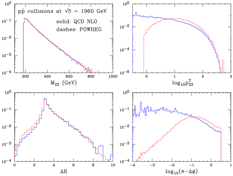
Figure 2: Comparison of four distributions computed according to the fixed order calculation and the POWHEG. On the vertical axes we report the cross sections in picobarns per bin. Energies are expressed in GeV.

We first notice that in the case of the invariant mass distributions the two calculations give identical results. On the contrary, the $\Delta\phi$ and $p^{\rm\scriptscriptstyle T}_{\rm\scriptscriptstyle ZZ}$ distributions are strongly affected by light parton emission, and indeed they display a sizable difference in the two calculations. In the fixed order calculation the divergences in the limit of soft/collinear light parton emissions are canceled when virtual corrections, that have strictly $p^{\rm\scriptscriptstyle T}_{\rm\scriptscriptstyle ZZ}=0$ and $\Delta\phi=\pi$, are included. However, the effect of virtual corrections is not seen in the $\Delta\phi$ and $p^{\rm\scriptscriptstyle T}_{\rm\scriptscriptstyle ZZ}$ plots, so that the fixed order calculation appears to yield logarithmically divergent integrals for $p^{\rm\scriptscriptstyle T}_{\rm\scriptscriptstyle ZZ}\to 0$ and $\Delta\phi\to\pi$. On the other hand, the POWHEG result is well behaved also in this region, since the no-radiation region is effectively suppressed by the form factor $\Delta_{q}(k_{\scriptscriptstyle\rm T})$ (see eq. (47)).

Our next task is to compare our full result with the only existing implementation of Monte Carlo generation of vector boson pairs with NLO accuracy, namely the MC@NLO program. The relevant plots are collected in figs. 3, 4, 5 for the Tevatron, and in figs. 6, 7, 8 for the LHC. The MC@NLO results are compared with POWHEG interfaced with HERWIG. According to the Les Houches interface prescription, the showering in the Monte Carlo is vetoed by assigning the $k_{\scriptscriptstyle\rm T}$ of the event generated by POWHEG to the variable SCALUP in the Les Houches common block. We find that the inclusion of the HERWIG shower determines only tiny changes with respect to the pure POWHEG output. It is easy to comment upon the outcome of this comparison: the two algorithms yield identical results. Minor differences are only seen in the $p^{\rm\scriptscriptstyle T}_{\rm\scriptscriptstyle ZZ}$ distribution; these can be easily attributed to the presence of a $k_{\scriptscriptstyle\rm T}$ hard cutoff, set at 0.8 GeV in the POWHEG.

It should be noted that the MC@NLO results have been computed using the scale choice suggested by the authors, namely

$$\mu^{2}={1\over 2}\left(\sqrt{p_{T1}^{2}+m_{\scriptscriptstyle Z}^{2}}+\sqrt{p_{T2}^{2}+m_{\scriptscriptstyle Z}^{2}}\right),$$ (99)

while the POWHEG results are obtained with the scale choices described at the beginning of this section. This difference has a negligible impact on the total cross section, but may affect some of the distributions.

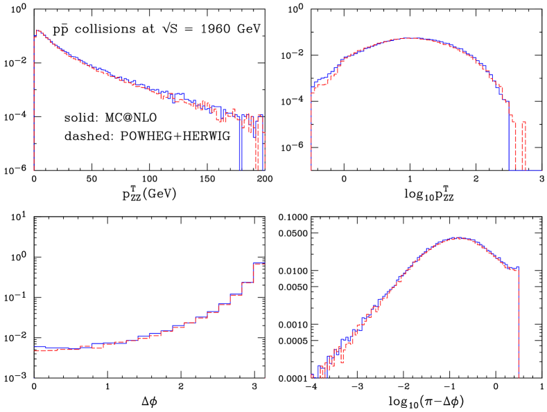
Figure 3: Comparison of four distributions computed according to MC@NLO and the POWHEG. On the vertical axes we report the cross sections in picobarns per bin. Energies are expressed in GeV.

The agreement between the two methods in the region of large transverse momentum radiation is expected, since both methods are in good agreement with the fixed-order calculation in this region. The region of soft radiation in the MC@NLO implementation is controlled by the HERWIG shower. We therefore conclude that our treatment of the soft region is consistent with the HERWIG implementation. We point out that HERWIG fully implements the procedure discussed at the end of Section 3 for the treatment of the strong coupling constant in the shower emission, as we also do.

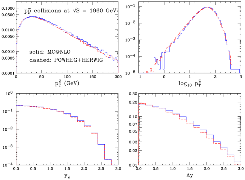
Figure 4: Comparison of four distributions computed according to MC@NLO and the POWHEG. On the vertical axes we report the cross sections in picobarns per bin. Energies are expressed in GeV.

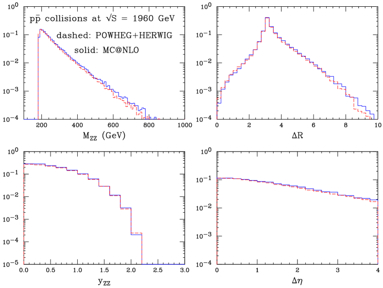
Figure 5: Comparison of four distributions computed according to MC@NLO and the POWHEG. On the vertical axes we report the cross sections in picobarns per bin. Energies are expressed in GeV.

Figure 6: Same as fig. 3 for the LHC.

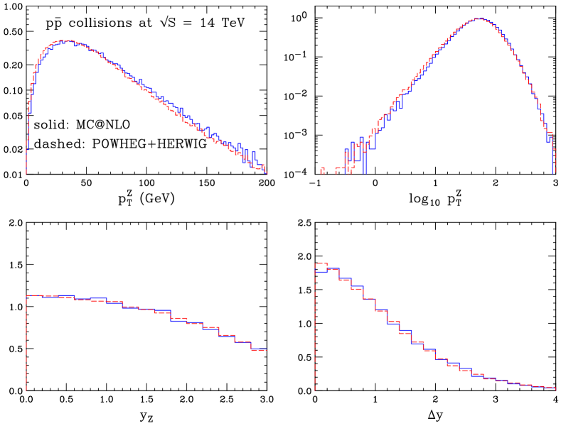
Figure 7: Same as fig. 4 for the LHC.

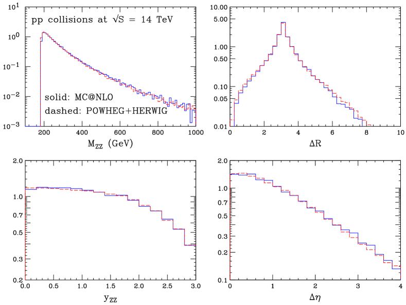
Figure 8: Same as fig. 5 for the LHC.

One of the main features of the POWHEG method is the possibility of interfacing its output to any shower Monte Carlo that implements the Les Houches interface for user-provided processes. This is possible with the popular Monte Carlo PYTHIA [19] since its version 6.3, which is based upon a $p_{\scriptscriptstyle\rm T}$-ordered shower algorithm. We thus interfaced POWHEG to PYTHIA and compared the results to the pure PYTHIA output, normalized to the POWHEG cross section. By inspection of fig. 9, relevant to the Tevatron configuration,

Figure 9: Comparison of four distributions computed according to PYTHIA and the POWHEG interfaced to PYTHIA.

we see that the POWHEG result appears to have a harder $p^{\rm\scriptscriptstyle T}_{\rm\scriptscriptstyle ZZ}$ spectrum, especially in the low $p^{\rm\scriptscriptstyle T}_{\rm\scriptscriptstyle ZZ}$ region. Correspondingly, the $\Delta\phi$ distribution obtained by POWHEG is also shifted away from the region $\Delta\phi\sim\pi$ with respect to the PYTHIA result. A detailed view of the small-$p^{\rm\scriptscriptstyle T}_{\rm\scriptscriptstyle ZZ}$ region is shown in fig. 10 for both the Tevatron and the LHC.

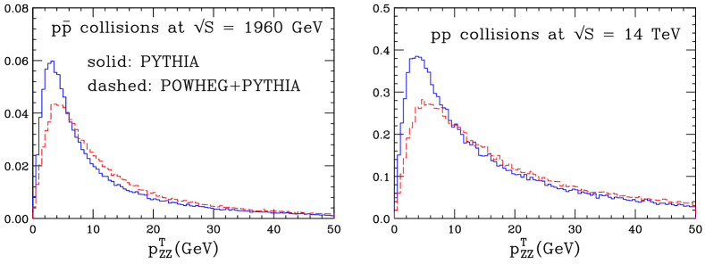
Figure 10: Comparison of the $p^{\rm\scriptscriptstyle T}_{\rm\scriptscriptstyle ZZ}$ distribution computed according to PYTHIA and the POWHEG interfaced to PYTHIA, for both the Tevatron and the LHC.

We see that the position of the peak in the $p^{\rm\scriptscriptstyle T}_{\rm\scriptscriptstyle ZZ}$ distribution is rather different in the two approaches. We have verified that also in this case, the effect of the PYTHIA showering in the POWHEG$+$PYTHIA result is negligible in the distributions we are considering. We thus infer that the same differences should appear when comparing PYTHIA with MC@NLO. This issue deserves further investigations, that are however beyond the purposes of the present work.

7 Conclusions

We have presented an explicit implementation of the method presented in ref. [5] for the construction of a Monte Carlo event generator with matrix elements accurate to next-to-leading order, and positive weights. The process we have considered is $Z$ pair production in hadron collisions, which is a process of intermediate complexity that involves initial-state radiation, and thus is a good testing ground for the applicability of the method to hadron collision processes.

One of the main achievements of the present work is the development of numerical techniques that are necessary for the practical implementation of the method proposed in ref. [5]. We have given here a full, detailed description of these techniques, so that all our results can in principle be reproduced by the interested reader.

The output of our generator is cast in the form of the Les Houches Interface for user provided processes [8], and thus easily interfaced to both the HERWIG and the PYTHIA shower Monte Carlo programs.

We have compared our result to the only existing program that can compute NLO corrected Shower Monte Carlo output in hadronic collisions, for a large set of observables, both for the Tevatron and the LHC. We have found an excellent agreement.

Our method can also be used as a standalone, alternative implementation of QCD corrections. As discussed in section 6, the interfacing to the SMC has negligible effects on the POWHEG distributions involving $ZZ$ observables. It may thus becomes convenient to compute these observable by using POWHEG as a standalone program. This has several advantages over the standard, fixed order QCD calculation, like positivity, and next-to-leading logarithmic accuracy in the small $k_{\scriptscriptstyle\rm T}$ region.

The extension of the present work to $WZ$ and $WW$ pair production is straightforward. Furthermore, the choice of kinematic variables adopted here can be easily extended to processes of Drell-Yan type, like single $W$ and $Z$ production, and Higgs production. We also believe that the method can be applied without major modifications to the case of heavy flavour production, where final state soft radiation is also present. The treatment of collinear final state radiation with the method of ref. [5] presents no difficulties, being in fact easier than the initial state radiation case. The formulation of the application of the method to general processes is under study.

In order to fully preserve double logarithmic accuracy in the POWHEG context, the Shower Monte Carlo to which the program is interfaced should generate consistently the needed soft radiation pattern. When using an angular ordered shower program, one needs to include additional soft radiation, that was named “truncated showers” in ref. [5]. Programs that generate soft radiation using dipole type formalisms [6, 7] may not require any further correction. At present, however, no such program is available that handles initial state radiation. These problems are left for future studies.

Acknowledgments: We thank Stefano Frixione for helpful discussions and suggestions, and Carlo Oleari for carefully reading the manuscript. We also thank Torbjörn Sjöstrand for clarifications on the use of PYTHIA.

Appendix A The hit-and-miss technique

In order to generate a set of continuous variables $x$ and an index $j=1,\ldots,m$, with a probability distribution proportional to $F_{j}(x)$, one first computes

$$F_{\rm tot}=\sum_{j}\int dx\,F_{j}(x)\,,\quad\quad F_{\rm max}=\max_{x}\sum_{j}F_{j}(x)\;.$$ (100)

Then, one generates a random value $x={\bar{x}}$ and a random number $0<n<1$ with flat distributions, and finds the smallest value $k$ such that

$$\sum_{j=1}^{k}F_{j}({\bar{x}})>n\,F_{\rm max}\;.$$ (101)

If such $k$ does not exist, the event is rejected; otherwise the set $j=k,x={\bar{x}}$ is accepted.

Appendix B From Monte Carlo integration to uniform generation

We want to to generate a set of values for the variables $x$ in a domain ${\cal D}$ with a distribution proportional to $F(x)$. We divide the integration range ${\cal D}$ into a set of hypercubes ${\cal D}_{i}$, with $i=1,\ldots,m$. For each hypercube we compute

$$F_{\rm tot}^{(i)}=\int_{{\cal D}_{i}}dx\,F(x)\,,\quad\quad F_{\rm max}^{(i)}=\max_{x\in{\cal D}_{i}}F(x)\,,\quad\quad F_{\rm tot}=\sum_{i=1}^{m}F_{\rm tot}^{(i)}\;.$$ (102)

In order to generate the $x$ values, we first choose the hypercube according to its probability: given a random number $0<n<1$ we find the minimum value $k$ such that

$$\sum_{j=1}^{k}F^{(j)}_{\rm tot}>n\,F_{\rm tot}\;.$$ (103)

Next we generate $x$ in the ${\cal D}_{k}$ hypercube using the hit-and-miss technique. It is clear that the efficiency of the generation improves by reducing the size (and thus increasing the number) of the hypercubes. Thus there will be a trade-off between speed and storage requirement in the computer implementation of this technique.

Appendix C The veto technique

Assume we want to generate values for a set of variables $x$, according to a distribution

$$P(x)=R(x)\,\exp\left[-\int d^{d}x^{\prime}\,R(x^{\prime})\,\theta(p(x^{\prime})-p(x))\right]\,,$$ (104)

where $p(x)\geq 0$. We assume that $R(x)$ is non-negative, and that the unconstrained integral is divergent. We observe that the probability distribution of $p(x)$ is an exact differential. Indeed,

$$\int d^{d}x\,P(x)\,\delta(p(x)-p) = \int d^{d}x\,R(x)\,\delta(p(x)-p)\,\exp\left[-\int d^{d}x^{\prime}\,R(x^{\prime})\,\theta(p(x^{\prime})-p)\right]$$ (105)

$$= {d\over dp}\Delta(p)\;,$$

where we have defined

$$\Delta(p)=\exp\left[-\int d^{d}x^{\prime}\,R(x^{\prime})\,\theta(p(x^{\prime})-p)\right]\;.$$ (106)

The function $\Delta(p)$ ranges between 0 and 1, because the integral in the exponent vanishes for $p\to+\infty$ and diverges to $+\infty$ for $p=0$. Hence, eq. (105) also shows that $P(x)$ is normalized to 1:

$$\int d^{d}x\,P(x)=\int_{0}^{+\infty}dp\int d^{d}x\,P(x)\,\delta(p(x)-p)=\Delta(\infty)-\Delta(0)=1\;.$$ (107)

In principle, the uniform generation of events is therefore straightforward: one generates a uniform random number $r$ between 0 and 1, solves the equation $\Delta(p)=r$ for $p$, and then generates values of $x$ on the surface $\delta(p(x)-p)$ with a distribution proportional to $R(x)\,\delta(p(x)-p)$.

In practice, however, the solution of the equation $\Delta(p)=r$ is in most cases very heavy from the numerical point of view. This difficulty can be overcome by means of the so-called vetoing method, which we now describe. We assume that there is a function $H(x)\geq R(x)$ for all $x$ values, and that

$$\Delta_{H}(p)=\exp\left[-\int d^{d}x^{\prime}\,H(x^{\prime})\,\theta(p(x^{\prime})-p)\right]\;$$ (108)

has a simple form, so that the solution of the equation $\Delta_{H}(p)=r$ and the generation of the distribution $H(x)\,\delta(p(x)-p)$ are reasonably simple. Then, we implement the following procedure:

1. Set $p_{\rm max}=\infty$.

2. Generate a flat random number $0<n<1$.

3. Solve the equation

   $${\Delta_{H}(p)\over\Delta_{H}(p_{\rm max})}=n$$ (109)

   for $p$ (a solution with $0<p<p_{\rm max}$ always exists for $0<n<1$).

4. Generate $x$ according to $H(x)\,\delta(p(x)-p)$.

5. Generate a new random number $n^{\prime}$.

6. If $n^{\prime}>R(x)/H(x)$ then the event is vetoed, we set $p_{\rm max}=p$, go to step 3 and continue; otherwise the event is accepted, and the procedure stops.

The resulting events are distributed according to eq. (104). The proof of this statement is simple but non-trivial. At the end of the vetoing procedure, the event distribution will be given by the sum of the distribution for the case in which there is no veto, there is one veto applied, two vetoes, etc.. The probability distribution of events generated with no veto applied is given by

$$P_{0}(x)=\int_{0}^{p_{\rm max}}dp_{1}\,{\Delta_{H}(p_{1})\over\Delta_{H}(p_{\rm max})}\,H(x)\,\delta(p(x)-p_{1}))\,{R(x)\over H(x)}\\ =R(x)\,\Delta_{H}(p(x))\,.$$

We have used the fact that $\Delta_{H}(p_{\rm max})=\Delta_{H}(\infty)=1$, and we have inserted a factor of $R(x)/H(x)$, corresponding to the acceptance probability.

When one veto is applied, we have

$$P_{1}(x) = \int_{0}^{p_{\rm max}}dp_{1}\,{\Delta_{H}(p_{1})\over\Delta_{H}(p_{\rm max})}\,\int d^{d}x_{1}\,H(x_{1})\,\delta(p(x_{1})-p_{1})\,\left(1-{R(x_{1})\over H(x_{1})}\right)\,$$ (110)

$$\int_{0}^{p_{1}}dp_{2}\,{\Delta_{H}(p_{2})\over\Delta_{H}(p_{1})}\,H(x)\,\delta(p(x)-p_{2}))\,{R(x)\over H(x)}$$

$$= R(x)\,\Delta_{H}(p(x))\,\int_{p(x)}^{+\infty}dp_{1}\,h(p_{1})\,,$$

where we have defined

$$h(p_{1})=\int d^{d}x_{1}\,H(x_{1})\,\delta(p(x_{1})-p_{1})\,\left(1-{R(x_{1})\over H(x_{1})}\right)\,.$$ (111)

The factor $1-R(x_{1})/H(x_{1})$ is the rejection probability, which must be inserted at each vetoed step. Note that the result is nonzero only for $p_{1}\geq p(x)$, because of the $\delta$ function in the $p_{2}$ integration. It will be useful to perform one more step explicitly; for two vetoes, we find

$$P_{2}(x) = \int_{0}^{p_{\rm max}}dp_{1}\,{\Delta_{H}(p_{1})\over\Delta_{H}(p_{\rm max})}\,h(p_{1})\int_{0}^{p_{1}}dp_{2}\,{\Delta_{H}(p_{2})\over\Delta_{H}(p_{1})}\,h(p_{2})$$ (112)

$$\int_{0}^{p_{2}}dp_{3}\,{\Delta_{H}(p_{3})\over\Delta_{H}(p_{2})}\,H(x)\,\delta(p(x)-p_{3}))\,{R(x)\over H(x)}$$

$$= R(x)\,\Delta_{H}(p(x))\,{1\over 2}\left[\int_{p(x)}^{+\infty}dp\,h(p)\right]^{2}\,,$$

where we have used symmetric integration. It is now easy to obtain the generic term of this infinite sum, namely the term with $n$ vetoes applied. We get

$$P_{n}(x)=\Delta_{H}(p(x))\,R(x)\,{1\over n!}\left[\int_{p(x)}^{+\infty}dp\,h(p)\right]^{n}\,.$$ (113)

The sum over $n$ yields

$$\sum_{n=0}^{\infty}P_{n}(x) = R(x)\,\Delta_{H}(p(x))\,\exp\left[\int_{p(x)}^{+\infty}dp\,h(p)\right]$$ (114)

$$= R(x)\,\Delta_{H}(p(x))\,\exp\left[\int d^{d}x^{\prime}\,[H(x^{\prime})-R(x^{\prime})]\,\theta(p(x^{\prime})-p(x))\right]$$

$$= R(x)\,\exp\left[-\int d^{d}x^{\prime}\,R(x^{\prime})\,\theta(p(x^{\prime})-p(x))\right]\,,$$

which is the announced result.

Appendix D Generation of events according to $\Delta_{q}^{(U)}$

The veto technique described in the previous Appendix can be employed to find the solution of eq. (88), which we reproduce here:

$$n={\Delta_{q}^{(U)}(v,p_{\scriptscriptstyle\rm T})\over\Delta_{q}^{(U)}(v,p_{\rm max})}$$ (115)

where $n$ is a random number between 0 and 1,

$$\Delta_{q}^{(U)}(v,p_{\scriptscriptstyle\rm T})=\exp\left[-\int U_{q}(v,r)\,\theta(k_{\scriptscriptstyle\rm T}(v,r)-p_{\scriptscriptstyle\rm T})\,d\Phi_{r}\right]\,;\qquad r=\{x,y,\theta_{2}\}$$ (116)

and

$$U_{q}(v,r)=N_{q}\,{\alpha_{s}(k_{\scriptscriptstyle\rm T}^{2}(v,r))\over(1-x)\,(1-y^{2})}\,.$$ (117)

Trading the variable $y$ for

$$k_{\scriptscriptstyle\rm T}^{2}=k_{\scriptscriptstyle\rm T}^{2}(v,r)={M_{\scriptscriptstyle ZZ}^{2}\over 4x}\,(1-x)^{2}(1-y^{2}),\qquad\left|y\right|=\sqrt{1-{4x\over(1-x)^{2}}{k_{\scriptscriptstyle\rm T}^{2}\over M_{\scriptscriptstyle ZZ}^{2}}}$$ (118)

we find

$$\int U_{q}(v,r)\,\theta(k_{\scriptscriptstyle\rm T}(v,r)-p_{\scriptscriptstyle\rm T})\,d\Phi_{r} = \int_{\rho}^{1}dx\int_{-1}^{1}dy\int_{0}^{\pi}d\theta_{2}\,U_{q}(v,r)\,\theta(k_{\scriptscriptstyle\rm T}(v,r)-p_{\scriptscriptstyle\rm T})$$ (119)

$$= \pi N_{q}\,\int_{\rho}^{x_{-}}dx\,\int_{p_{\scriptscriptstyle\rm T}^{2}}^{{k_{\scriptscriptstyle\rm T}^{2}}_{\rm max}}{dk_{\scriptscriptstyle\rm T}^{2}\over k_{\scriptscriptstyle\rm T}^{2}}\,{\alpha_{s}(k_{\scriptscriptstyle\rm T}^{2})\over\sqrt{(x_{+}-x)(x_{-}-x)}}\,,$$

where

$$\rho={M_{\scriptscriptstyle ZZ}^{2}\over S};\qquad{k_{\scriptscriptstyle\rm T}^{2}}_{\rm max}={S\over 4}(1-\rho)^{2};\qquad x_{\pm}=\left(\sqrt{1+{k_{\scriptscriptstyle\rm T}^{2}\over M_{\scriptscriptstyle ZZ}^{2}}}\pm{k_{\scriptscriptstyle\rm T}\over M_{\scriptscriptstyle ZZ}}\right)^{2}.$$ (120)

We have supplied an extra factor of 2 to account for the fact that each value of $k_{\scriptscriptstyle\rm T}^{2}$ corresponds to two values of $y$. The integration range for $x$ is limited by the definition $x=M_{\scriptscriptstyle ZZ}^{2}/s$, and by the condition $s\leq S$. The $x$ integration can be performed with the variable change $\xi=\sqrt{x_{+}-x}+\sqrt{x_{-}-x}$. We get

$$\int U_{q}(v,r)\,\theta(k_{\scriptscriptstyle\rm T}(v,r)-p_{\scriptscriptstyle\rm T})\,d\Phi_{r}=\int_{p_{\scriptscriptstyle\rm T}^{2}}^{{k_{\scriptscriptstyle\rm T}^{2}}_{\rm max}}{dk_{\scriptscriptstyle\rm T}^{2}\over k_{\scriptscriptstyle\rm T}^{2}}\,V(k_{\scriptscriptstyle\rm T}^{2})\,,$$ (121)

where

$$V(k_{\scriptscriptstyle\rm T}^{2})=\pi N_{q}\,\alpha_{s}(k_{\scriptscriptstyle\rm T}^{2})\,\log{\sqrt{x_{+}-\rho}+\sqrt{x_{-}-\rho}\over\sqrt{x_{+}-\rho}-\sqrt{x_{-}-\rho}}\,.$$ (122)

We now observe that

$$\log{\sqrt{x_{+}-\rho}+\sqrt{x_{-}-\rho}\over\sqrt{x_{+}-\rho}-\sqrt{x_{-}-\rho}}\leq\log{\sqrt{x_{+}}+\sqrt{x_{-}}\over\sqrt{x_{+}}-\sqrt{x_{-}}}={1\over 2}\log{k_{\scriptscriptstyle\rm T}^{2}+M_{\scriptscriptstyle ZZ}^{2}\over k_{\scriptscriptstyle\rm T}^{2}}\leq{1\over 2}\log{q^{2}\over k_{\scriptscriptstyle\rm T}^{2}}\,$$ (123)

where

$$q^{2}={k_{\scriptscriptstyle\rm T}^{2}}_{\rm max}+M_{\scriptscriptstyle ZZ}^{2}={S\over 4}(1+\rho)^{2}.$$ (124)

Furthermore,

$$\alpha_{s}(k_{\scriptscriptstyle\rm T}^{2})={\alpha_{s}(k_{\scriptscriptstyle\rm T}^{2})\over\alpha_{s}^{0}(k_{\scriptscriptstyle\rm T}^{2})}\,\alpha_{s}^{0}(k_{\scriptscriptstyle\rm T}^{2})\leq\alpha_{s}^{0}(k_{\scriptscriptstyle\rm T}^{2})\,,$$ (125)

where $\alpha_{s}^{0}(k_{\scriptscriptstyle\rm T}^{2})$ is the leading-log expression of the running coupling,

$$\alpha_{s}^{0}(k_{\scriptscriptstyle\rm T}^{2})={1\over\beta_{0}\,\log{k_{\scriptscriptstyle\rm T}^{2}\over\Lambda^{2}}}\,.$$ (126)

Hence

$$V(k_{\scriptscriptstyle\rm T}^{2})\leq\tilde{V}(k_{\scriptscriptstyle\rm T}^{2})={\pi N_{q}\over 2\beta_{0}}\,{1\over\log{k_{\scriptscriptstyle\rm T}^{2}\over\Lambda^{2}}}\,\log\log{q^{2}\over k_{\scriptscriptstyle\rm T}^{2}}\,.$$ (127)

The $k_{\scriptscriptstyle\rm T}^{2}$ integral of $\tilde{V}$ can be performed analytically:

$$\int_{p_{\scriptscriptstyle\rm T}^{2}}^{{k_{\scriptscriptstyle\rm T}^{2}}_{\rm max}}{dk_{\scriptscriptstyle\rm T}^{2}\over k_{\scriptscriptstyle\rm T}^{2}}\,\tilde{V}(k_{\scriptscriptstyle\rm T}^{2})={\pi N_{q}\over 2\beta_{0}}\left[\log{q^{2}\over\Lambda^{2}}\log{\log{{k_{\scriptscriptstyle\rm T}^{2}}_{\rm max}\over\Lambda^{2}}\over\log{p_{\scriptscriptstyle\rm T}^{2}\over\Lambda^{2}}}-\log{{k_{\scriptscriptstyle\rm T}^{2}}_{\rm max}\over p_{\scriptscriptstyle\rm T}^{2}}\right].$$ (128)

We now proceed as follows:

1. We set $p_{\rm max}={k_{\scriptscriptstyle\rm T}}_{\rm max}$.

2. We generate uniformly a random number $n$, $0\leq n\leq 1$, and we solve numerically the equation

   $$n={\Delta^{(\tilde{V})}(p_{\scriptscriptstyle\rm T})\over\Delta^{(\tilde{V})}(p_{\rm max})};\qquad{\Delta^{(\tilde{V})}(p_{\scriptscriptstyle\rm T})}=\exp\left[-\int_{p_{\scriptscriptstyle\rm T}^{2}}^{{k_{\scriptscriptstyle\rm T}^{2}}_{\rm max}}{dk_{\scriptscriptstyle\rm T}^{2}\over k_{\scriptscriptstyle\rm T}^{2}}\,\tilde{V}(k_{\scriptscriptstyle\rm T}^{2})\right]$$ (129)

   for $p_{\scriptscriptstyle\rm T}$.

3. We generate a second random number $n^{\prime}$ between 0 and 1; if $n^{\prime}<V(p_{\scriptscriptstyle\rm T}^{2})/\tilde{V}(p_{\scriptscriptstyle\rm T}^{2})$ we accept the event, otherwise we set $p_{\rm max}=p_{\scriptscriptstyle\rm T}$ and we return to step 2.

References

• [1] S. Frixione and B. R. Webber, JHEP 0206 (2002) 029, hep-ph/0204244;
S. Frixione and B. R. Webber, hep-ph/0207182.
• [2] S. Frixione, P. Nason and B. R. Webber, JHEP 0308 (2003) 007, hep-ph/0305252.
• [3] S. Frixione, E. Laenen, P. Motylinski and B. R. Webber, hep-ph/0512250.
• [4] HERWIG 6.5, G. Corcella etal, JHEP 0101 (2001) 010, hep-ph/0011363; hep-ph/0210213.
• [5] P. Nason, JHEP 0411 (2004) 040, hep-ph/0409146.
• [6] G. Gustafson and U. Pettersson, Nucl. Phys. B306 (1988) 746.
• [7] U. Pettersson, LU TP 88-5 (1988);
L. Lönnblad and U. Pettersson, LU TP 88-15 (1988);
L. Lönnblad, Computer Physics Commun. 71 (1992) 15.
• [8] E. Boos et al., hep-ph/0109068.
• [9] B. Mele, P. Nason and G. Ridolfi, Nucl. Phys. B 357 (1991) 409.
• [10] L. J. Dixon, Z. Kunszt and A. Signer, Phys. Rev. D 60 (1999) 114037, hep-ph/9907305.
• [11] J. M. Campbell and R. K. Ellis, Phys. Rev. D 60 (1999) 113006, hep-ph/9905386.
• [12] Y. L. Dokshitzer, D. Diakonov and S. I. Troian, Phys. Rept.  58 (1980) 269.
• [13] R. K. Ellis and S. Veseli, Nucl. Phys. B 511 (1998) 649, hep-ph/9706526.
• [14] S. Frixione, P. Nason and G. Ridolfi, Nucl. Phys. B 542 (1999) 311, hep-ph/9809367.
• [15] S. Catani, B. R. Webber and G. Marchesini, Nucl. Phys. B 349 (1991) 635.
• [16] M. A. Dobbs et al., hep-ph/0403045.
• [17] S. Kawabata, Comput. Phys. Commun.  88 (1995) 309.
• [18] J. Pumplin, A. Belyaev, J. Huston, D. Stump and W. K. Tung, JHEP 0602 (2006) 032, hep-ph/0512167.
• [19] T. Sjostrand, S. Mrenna and P. Skands, JHEP 05 (2006) 026, hep-ph/0603175.
• [20] Z. Nagy and D. E. Soper, JHEP 0510 (2005) 024, hep-ph/0503053.