Once again about the reaction $\phi(1020)\to\gamma\pi\pi$

Abstract

Gauge invariance constraints and analytical properties of the amplitudes $e^{+}e^{-}\to\gamma\pi\pi$ and $\phi(1020)\to\gamma\pi\pi$ are discussed in line with the criticism of N.N. Achasov in hep-ph/0606003. I show that the formulae of our paper (Yad. Fiz. 68 1614 (2005) [PAN 68 1554 (2005)], hep-ph/0403123) have nothing common with those N.N. Achasov claims to be ours - his criticism is therefore misplaced.

PACS numbers: 12.39.-x , 13.40.Hq , 13.65.+i

In the paper [1], we investigated the reactions $e^{+}e^{-}\to\gamma\pi\pi$, $\phi(1020)\to\gamma\pi\pi$ and came to the conclusion that available experimental data do not contradict the assumed $q\bar{q}$ structure of $f_{0}(980)$. This paper was recently criticized by N.N. Achasov in [2]. He wrote that ”the realization of gauge invariance as a concequent of cancellation between the $\phi(1020)\to\gamma f_{0}(980)\to\gamma\pi^{0}\pi^{0}$ resonance contribution and background one, suggested in Ref. [1], is misleading.”

In this short note, I would like to remind the logic of reasoning in Ref. [1] and, comparing it with that of N.N. Achasov [2], to argue in which points the logic of N.N. Achasov is incorrect.

1 The logic of paper [1]

Let us start with the general formula for the transition amplitude $e^{+}e^{-}\to\gamma\pi\pi$ assuming that the $e^{+}e^{-}$ system is in the $1^{--}(V)$ state, $\pi\pi$ system in the $I=0,0^{++}(S)$ state and the photon is real (eq. (20) in [1]):

$$A_{\mu\alpha}^{(V\to\gamma S)}(s_{V},s_{S},q^{2}=0)\,=\,\left(g_{\mu\alpha}-\frac{2q_{\mu}P_{V\alpha}}{s_{V}-s_{S}}\right)A_{V\to\gamma S}(s_{V},s_{S},0)\ .$$ (1)

The indices $\mu$ and $\alpha$ refer to the initial vector state (total momentum $P_{V}$ and $P_{V}^{2}=s_{V}$) and photon (momentum $q$ and $q^{2}=0$). We have $(P_{V}-q)^{2}=s_{S}$ and $(P_{V}q)=(s_{V}-s_{S})/2$. The spin operator $[g_{\mu\alpha}-2q_{\mu}P_{V\alpha}/(s_{V}-s_{S})]$ is gauge invariant:

$$[g_{\mu\alpha}-2q_{\mu}P_{V\alpha}/(s_{V}-s_{S})]q_{\alpha}=0,\quad P_{V\mu}[g_{\mu\alpha}-2q_{\mu}P_{V\alpha}/(s_{V}-s_{S})]=0.$$

The requirement of analyticity (absence of the pole at $s_{V}=s_{S}$) leads to the condition (eq. (21) in [1]):

$$\bigg{[}A_{V\to\gamma S}(s_{V},s_{S},0)\bigg{]}_{s_{V}\to s_{S}}\ \sim\ (s_{V}-s_{S})\,,$$ (2)

that is the threshold theorem for the transition amplitude $V\to\gamma S$.

It should be now emphasized that the form of the spin operator in eq.(1), $[g_{\mu\alpha}-2q_{\mu}P_{V\alpha}/(s_{V}-s_{S})]$, is not unique. Alternatively, one can write the spin factor as a metric tensor $g^{\perp\perp}_{\mu\alpha}$ which works in the space orthogonal to $P_{V}$ and $q$, i.e. $P_{V\mu}g^{\perp\perp}_{\mu\alpha}=0$ and $g^{\perp\perp}_{\mu\alpha}\,q_{\alpha}=0$. Ambiguities in choice of the spin operator for the process $V\to\gamma S$ are due to the fact that the difference

$$g^{\perp\perp}_{\mu\alpha}-[g_{\mu\alpha}-2q_{\mu}P_{V\alpha}/(s_{V}-s_{S})]$$

is the nilpotent operator, for the detail see [3, 4] and eqs. (22)-(25) in [1]. (Note that the use of the operator $g^{\perp\perp}_{\mu\alpha}$ was also criticized by N.N. Achasov [5] but he did not pay attention to the presence of nilpotent operators).

Figure 1: Process $e^{+}e^{-}\to\gamma\pi\pi$: residues in the $e^{+}e^{-}$ and $\pi\pi$ channels determine the $\phi\to\gamma f_{0}$ amplitude.

1.1 Transitions $e^{+}e^{-}\to\gamma\pi\pi$ , $\phi\to\gamma f_{0}$ and $\phi\to\gamma\pi\pi$ .

The amplitude of the transition $e^{+}e^{-}\to\gamma\pi\pi$ determines the amplitudes $\phi\to\gamma f_{0}$ and $\phi\to\gamma\pi\pi$ as corresponding residues of the pole terms.

1.1.1 The amplitude $e^{+}e^{-}\to\gamma\pi\pi$: the pole and background terms

The $A_{\phi\to\gamma f_{0}}$ amplitude is defined as the amplitude residue of the corresponding double-pole term in the amplitude $e^{+}e^{-}\to\gamma\pi\pi$. For $e^{+}e^{-}\to\gamma\pi\pi$, see Fig. 1, the amplitude with singled out double-pole term reads (eq. (26) in [1]):

$$A^{(e^{+}e^{-}\to\gamma\pi\pi)}_{\mu\alpha}(s_{V},s_{S},0)\ =\left(g_{\mu\alpha}-\frac{2q_{\mu}P_{V\alpha}}{s_{V}-s_{S}}\right)\times$$

$$\times\left[G_{e^{+}e^{-}\to\phi}\ \frac{A_{\phi\to\gamma f_{0}}(m^{2}_{\phi},m^{2}_{f_{0}},0)}{(s_{V}-m^{2}_{\phi})(s_{S}-m^{2}_{f_{0}})}\ g_{f_{0}\to\pi\pi}+B(s_{V},s_{S},0)\right].$$ (3)

Here, $A(m^{2}_{\phi},m^{2}_{f_{0}},0)$, up to the factors $G_{e^{+}e^{-}\to\phi}$ and $g_{f_{0}\to\pi\pi}$, is the residue in the amplitude poles $s_{V}=m^{2}_{\phi}$ and $s_{S}=m^{2}_{f_{0}}$: just this value supplies us with the transition amplitude for the reaction with bound states, $\phi\to\gamma f_{0}$.

In eq. (3), we deal with the double-pole term only. The amplitude $B(s_{V},s_{S},0)$ may contain single-pole terms too. Writing down all pole terms, one has:

$$A^{(e^{+}e^{-}\to\gamma\pi\pi)}_{\mu\alpha}(s_{V},s_{S},0)\ =\left(g_{\mu\alpha}-\frac{2q_{\mu}P_{V\alpha}}{s_{V}-s_{S}}\right)\left[G_{e^{+}e^{-}\to\phi}\ \frac{A_{\phi\to\gamma f_{0}}(m^{2}_{\phi},m^{2}_{f_{0}},0)}{(s_{V}-m^{2}_{\phi})(s_{S}-m^{2}_{f_{0}})}\ g_{f_{0}\to\pi\pi}+\right.$$

$$\left.+G_{e^{+}e^{-}\to\phi}\ \frac{B_{\phi}(m^{2}_{\phi},s_{S},0)}{s_{V}-m^{2}_{\phi}}+\frac{B_{f_{0}}(s_{V},m^{2}_{f_{0}},0)}{s_{S}-m^{2}_{f_{0}}}\ g_{f_{0}\to\pi\pi}+B_{0}(s_{V},s_{S},0)\right].$$ (4)

The threshold theorem (2) for the amplitude (4) reads:

$$\left[G_{e^{+}e^{-}\to\phi}\ \frac{A_{\phi\to\gamma f_{0}}(m^{2}_{\phi},m^{2}_{f_{0}},0)}{(s_{V}-m^{2}_{\phi})(s_{V}-m^{2}_{f_{0}})}\ g_{f_{0}\to\pi\pi}+\right.$$

$$\left.+G_{e^{+}e^{-}\to\phi}\ \frac{B_{\phi}(m^{2}_{\phi},s_{V},0)}{s_{V}-m^{2}_{\phi}}+\frac{B_{f_{0}}(s_{V},m^{2}_{f_{0}},0)}{s_{V}-m^{2}_{f_{0}}}\ g_{f_{0}\to\pi\pi}+B_{0}(s_{V},s_{V},0)\right]=0\,.$$ (5)

1.1.2 The $\phi\to\gamma f_{0}$ amplitude

If we deal with stable composite particles, in other words, if $\phi$ and $f_{0}$ can be included into the set of fields $|in\rangle$ and $\langle out|$, the transition amplitude $\phi\to\gamma f_{0}$ can be written in the form similar to (1) (see eq. (27) in [1]):

$$A^{(\phi\to\gamma f_{0})}_{\mu\alpha}(m^{2}_{\phi},m^{2}_{f_{0}},0)\ =\left(g_{\mu\alpha}-\frac{2q_{\mu}P_{\phi\alpha}}{m^{2}_{\phi}-m^{2}_{f_{0}}}\right)A_{\phi\to\gamma f_{0}}\left(m^{2}_{\phi},m^{2}_{f_{0}},0\right).$$ (6)

Here, we have substituted $P_{V}\to P_{\phi}$ where

$$P_{\phi}^{2}=m^{2}_{\phi},\quad(P_{\phi}-q)^{2}=m^{2}_{f_{0}},\quad q^{2}=0.$$

For $A_{\phi\to\gamma f_{0}}\left(m^{2}_{\phi},m^{2}_{f_{0}},0\right)$, the threshold theorem reads (eq. (28) in [1]):

$$\left[A_{\phi\to\gamma f_{0}}(m^{2}_{\phi},m^{2}_{f_{0}},0)\right]_{m^{2}_{\phi}\to m^{2}_{f_{0}}}\ \sim\ (m^{2}_{\phi}-m^{2}_{f_{0}})\ ,$$ (7)

that means that the threshold theorem of eq. (7) reveals itself as a requirement of analyticity of the amplitude (6).

1.1.3 The $\phi\to\gamma\pi\pi$ amplitude

To describe the reaction $\phi\to\gamma\pi\pi$ considering $\phi$ as a stable particle, one needs to separate from (4) the pole factors: $\sim(s_{V}-m^{2}_{\phi})^{-1}$. The amplitude $\phi\to\gamma\pi\pi$ is the residue in the pole $s_{V}=m^{2}_{\phi}$:

$$A^{(\phi\to\gamma\pi\pi)}_{\mu\alpha}(m^{2}_{\phi},s_{S},0)\ =\left(g_{\mu\alpha}-\frac{2q_{\mu}P_{\phi\alpha}}{m^{2}_{\phi}-s_{S}}\right)\left[\frac{A_{\phi\to\gamma f_{0}}(m^{2}_{\phi},m^{2}_{f_{0}},0)}{s_{S}-m^{2}_{f_{0}}}\ g_{f_{0}\to\pi\pi}+B_{\phi}(m^{2}_{\phi},s_{S},0)\right],$$ (8)

where

$$P_{\phi}^{2}=m^{2}_{\phi},\quad(P_{\phi}-q)^{2}=s_{S},\quad q^{2}=0.$$

Let us emphasize once more that $B_{\phi}(m^{2}_{\phi},s_{S},0)$ does not contain pole terms and $m_{\phi}$ is fixed ($m_{\phi}=1020$ MeV).

The analyticity condition reads:

$$\left[\frac{A_{\phi\to\gamma f_{0}}(m^{2}_{\phi},m^{2}_{f_{0}},0)}{s_{S}-m^{2}_{f_{0}}}\ g_{f_{0}\to\pi\pi}+B_{\phi}(m^{2}_{\phi},s_{S},0)\right]_{s_{S}\to m^{2}_{\phi}}\sim(s_{S}-m^{2}_{\phi}).$$ (9)

1.2 Example of idealistic description of $\phi(1020)\to\gamma\pi\pi$

To make clear our way of calculations, let us consider the idealistic case: the $f_{0}$ is a standard Breit-Wigner resonance, while $K\bar{K}$ channel is stongly supressed in the region under consideration and may be neglected. The $\phi$ is considered as a stable particle (the width of $\phi(1020)$ is small).

In this case, the $\phi\to\gamma\pi\pi$ amplitude is given by eq. (8), with

$$m_{f_{0}}^{2}=M_{0}^{2}-i\Gamma M_{0}\ .$$ (10)

To be illustrative, let us rewrite (8) extracting the Breit-Wigner resonance pole explicitly:

$$A^{(\phi\to\gamma\pi\pi)}_{\mu\alpha}(m^{2}_{\phi},s_{S},0)\ =\left(g_{\mu\alpha}-\frac{2q_{\mu}P_{\phi\alpha}}{m^{2}_{\phi}-s_{S}}\right)\left[\frac{A_{\phi\to\gamma f_{0}}(m^{2}_{\phi},m_{f_{0}}^{2},0)}{s_{S}-M_{0}^{2}+i\Gamma M_{0}}\ g_{f_{0}\to\pi\pi}+B_{\phi}(m^{2}_{\phi},s_{S},0)\right],$$ (11)

Recall that $B_{\phi}(m^{2}_{\phi},s_{S},0)$ is the background contribution, i.e. it does not contain the pole term related to $f_{0}(980)$ and $m_{\phi}$ is fixed, $m_{\phi}=1020$ MeV. In the fitting procedure, $B_{\phi}(m^{2}_{\phi},s_{S},0)$ can be approximated by a smooth term or as a contribution of other poles (for example, such as $\sigma$). The fitting to the parameters of $B_{\phi}(m^{2}_{\phi},s_{S},0)$ should be carried out under two constraints:

$$\left(\frac{A_{\phi\to\gamma f_{0}}(m^{2}_{\phi},m^{2}_{f_{0}},0)}{s_{S}-M_{0}^{2}+i\Gamma M_{0}}\ g_{f_{0}\to\pi\pi}+B_{\phi}(m^{2}_{\phi},s_{S},0)\right)=$$

$$=\left|\frac{A_{\phi\to\gamma f_{0}}(m^{2}_{\phi},m^{2}_{f_{0}},0)}{s_{S}-M_{0}^{2}+i\Gamma M_{0}}\ g_{f_{0}\to\pi\pi}+B_{\phi}(m^{2}_{\phi},s_{S},0)\right|\exp{\left(i\delta_{0}^{0}(s_{S})\right)}$$ (12)

and

$$\frac{A_{\phi\to\gamma f_{0}}(m^{2}_{\phi},m^{2}_{f_{0}},0)}{m^{2}_{\phi}-M_{0}^{2}+i\Gamma M_{0}}\ g_{f_{0}\to\pi\pi}+B_{\phi}(m^{2}_{\phi},m^{2}_{\phi},0)=0\ .$$ (13)

The factor $\exp{\left(i\delta_{0}^{0}(s_{S})\right)}$, where $\delta_{0}^{0}(s_{S})$ is the $\pi\pi$ scattering phase shift, appears in (12) because of the final state interactions of pions, while the condition (13) results from the threshold theorem (9).

1.3 Description of the reaction $\phi(1020)\to\gamma\pi\pi$ in paper [1]

The vector meson $\phi(1020)$ has rather small decay width, $\Gamma_{\phi(1020)}\simeq 4.5\,$MeV; from this point of view there is no doubt that treating $\phi(1020)$ as a stable particle is reasonable. As to $f_{0}(980)$, the picture is not so determinate. In the PDG compilation [6], the $f_{0}(980)$ width is given in the interval $40\leq\Gamma_{f_{0}(980)}\leq 100\,$MeV, and the width uncertainty is related not to the data unaccuracy (experimental data are rather good) but is due to a vague definition of the width.

Figure 2: Complex-$M$ plane and location of the poles corresponding to $f_{0}(980)$; the cut related to the $K\bar{K}$ threshold is shown as a broken solid line (here we denote $M=\sqrt{s_{S}}$).

The definition of the $f_{0}(980)$ width is aggravated by the $K\bar{K}$ threshold singularity that leads to the existence of two, not one, poles. According to the $K$-matrix analyses [8, 9], there are two poles in the $(IJ^{PC}=00^{++})$-wave at $s\sim 1.0$ GeV²,

$$M_{I}\simeq 1.020-i0.040\mbox{ GeV },\quad M_{II}\simeq 0.960-i0.200\mbox{ GeV },$$ (14)

which are located on different complex-$M$ sheets related to the $K\bar{K}$-threshold, see Fig. 2.

A significant trait of the $K$-matrix analysis is that it also gives us, along with the characteristics of real resonances, the positions of levels before the onset of the decay channels, i.e. it determines the bare states. In addition, the $K$-matrix analysis allows us to observe the transform of bare states into real resonances. In Fig. 3, one can see such a transform of the $00^{++}$-amplitude poles by switching off the decays $f_{0}\to\pi\pi,K\bar{K},\eta\eta,\eta\eta^{\prime},\pi\pi\pi\pi$. One may see that, after switching off the decay channels, the $f_{0}(980)$ turns into stable state, approximately 300 MeV lower:

$$f_{0}(980)\ \longrightarrow\ f^{bare}_{0}(700\pm 100)\ .$$ (15)

Figure 3: Complex-$M$ plane: trajectories of poles corresponding to the states $f_{0}(980)$, $f_{0}(1300)$, $f_{0}(1500)$, $f_{0}(1750)$, $f_{0}(1200-1600)$ within a uniform onset of the decay channels.

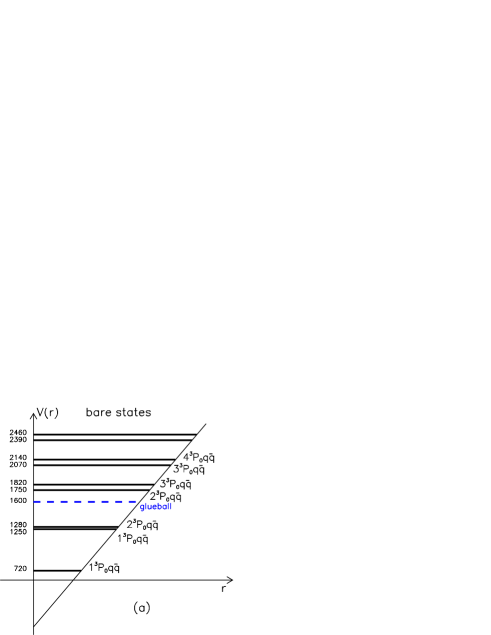
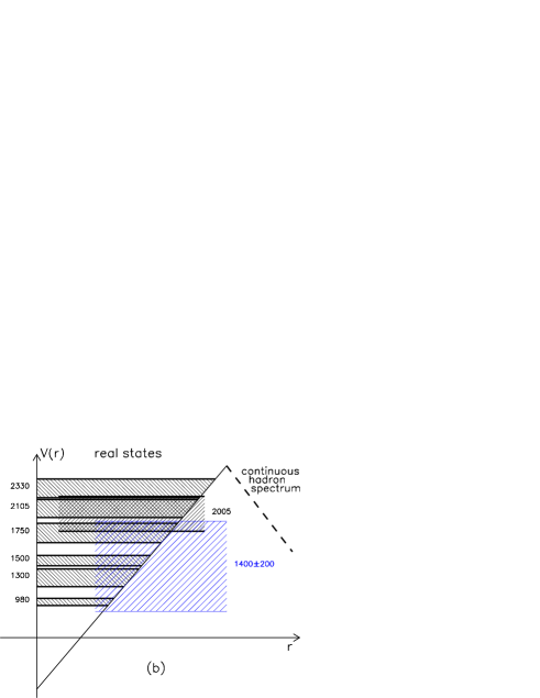
Figure 4: The $f_{0}$-levels in the potential well depending on the onset of the decay channels: bare states (a) and real resonances (b).

The transform of bare states into real resonances may be illustrated by Fig. 4 for the levels in the potential well: bare states are the levels in a well with impenetrable wall (Fig. 4a); at the onset of the decay channels (under-barrier transitions, Fig. 4b) the stable levels transform into real resonances. Note, that in this process one resonance (in the case of the $00^{++}$ states, it is gluonium) accumulates the widths of the neighbouring resonances thus becoming the broad state (the effect of accumulation of widths was firstly seen in nucler physics [7]).

The $K$-matrix amplitude of the $00^{++}$-wave reconstructed in [8] gives us the possibility to trace the evolution of the transition form factor $\phi(1020)\to\gamma f^{bare}_{0}(700\pm 100)$ during the transformation of the bare state $f^{bare}_{0}(700\pm 100)$ into the $f_{0}(980)$ resonance. Using the diagrammatic language, one can say that the evolution of the form factor $F^{(bare)}_{\phi\to\gamma f_{0}}$ is due to the processes shown in Fig. 5: $\phi$-meson goes into $f^{bare}_{0}(n)$, with the emission of the photon, then $f^{bare}_{0}(n)$ decays into mesons $f^{bare}_{0}(n)\to h_{a}h_{a}=\pi\pi$, $K\bar{K}$, $\eta\eta$, $\eta\eta^{\prime}$, $\pi\pi\pi\pi$. The decay yields may rescatter thus coming to final states.

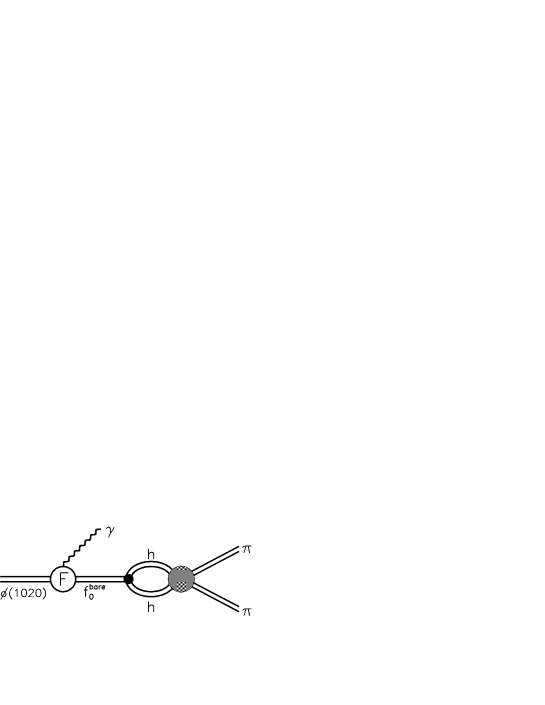
Figure 5: Diagram for the transition $\phi(1020)\to\gamma\pi\pi$ with final state interaction taken in terms of the K-matrix representation (the right-hand side block $hh\to\pi\pi$).

With the use of the K-matrix technique, the amplitude $\phi(1020)\to\gamma\pi\pi$ is given by eq. (8) with the following replacement (see Fig. 5):

$$\left[\frac{A_{\phi\to\gamma f_{0}}(m^{2}_{\phi},m^{2}_{f_{0}},0)}{s_{S}-m^{2}_{f_{0}}}\ g_{f_{0}\to\pi\pi}+B_{\phi}(m^{2}_{\phi},s_{S},0)\right]\longrightarrow$$ (16)

$$\longrightarrow\sum_{a}\left(\sum_{n}\frac{F^{(bare)}_{\phi(1020)\to\gamma f_{0}^{bare}(n)}\,g^{bare}_{a}(n)}{M^{2}_{n}-s_{S}}+b_{a}(s_{S})\right)\left(\frac{1}{1-i\hat{\rho}(s_{S})\hat{K}(s_{S})}\right)_{a,\pi\pi}\ ,$$

where the $K$-matrix elements $K_{ab}(s_{S})$ contain the poles corresponding to bare states:

$$K_{ab}(s)=\sum_{n}\frac{g^{bare}_{a}(n)\,g^{bare}_{b}(n)}{M^{2}_{n}-s_{S}}+f_{ab}(s_{S}).$$ (17)

Here $M_{n}$ is the mass of bare state, $g^{bare}_{a}(n)$ is the coupling for the transition $f^{bare}_{0}(n)\to a$, where

$$a=\pi\pi,\ K\bar{K},\ \eta\eta,\ \eta\eta^{\prime},\ \pi\pi\pi\pi.$$ (18)

The matrix element $(1-i\hat{\rho}(s)\hat{K}(s_{S}))^{-1}$ takes into account of the rescattering of the formed mesons. Here $\hat{\rho}(s_{S})$ is the diagonal matrix of phase spaces for hadronic states (for example, for the $\pi\pi$ system it reads: $\rho_{\pi\pi}(s_{S})=\sqrt{(s_{S}-4m^{2}_{\pi})/s_{S}}$ ). The functions $b_{a}(s_{S})$ and $f_{ab}(s)$ describe background contributions, they are smooth ones in the right-hand side half-plane, at Re$\,s_{S}>0$.

The formulae (16) and (17) are presented in [1] (eqs. (46),(47)), with the renotation $s_{S}\to s$.

To be scrupulous, let us present the amplitude $\phi(1020)\to\gamma\pi\pi$ explicitly:

$$A^{(\phi\to\gamma\pi\pi)}_{\mu\alpha}(m^{2}_{\phi},s_{S},0)\ =\left(g_{\mu\alpha}-\frac{2q_{\mu}P_{\phi\alpha}}{m^{2}_{\phi}-s_{S}}\right)\times$$

$$\times\left[\sum_{a}\left(\sum_{n}\frac{F^{(bare)}_{\phi(1020)\to\gamma f_{0}^{bare}(n)}\,g^{bare}_{a}(n)}{M^{2}_{n}-s_{S}}+b_{a}(s_{S})\right)\left(\frac{1}{1-i\hat{\rho}(s_{S})\hat{K}(s_{S})}\right)_{a,\pi\pi}\right]\ .$$ (19)

Therefore, the threshold condition reads:

$$\left[\sum_{a}\left(\sum_{n}\frac{F^{(bare)}_{\phi(1020)\to\gamma f_{0}^{bare}(n)}\,g^{bare}_{a}(n)}{M^{2}_{n}-s_{S}}+b_{a}(s_{S})\right)\left(\frac{1}{1-i\hat{\rho}(s_{S})\hat{K}(s_{S})}\right)_{a,\pi\pi}\right]_{s_{S}\to m^{2}_{\phi}}\sim m^{2}_{\phi}-s_{S}\ .$$ (20)

The fitting procedure of the reaction $\phi\to\gamma\pi\pi$ should be performed with the threshold constraint only:

$$\left[\sum_{a}\left(\sum_{n}\frac{F^{(bare)}_{\phi(1020)\to\gamma f_{0}^{bare}(n)}}{M^{2}_{n}-m^{2}_{\phi}}\,g^{bare}_{a}(n)+b_{a}(m^{2}_{\phi})\right)\left(\frac{1}{1-i\hat{\rho}(m^{2}_{\phi})\hat{K}(m^{2}_{\phi})}\right)_{a,\pi\pi}\right]=0$$ (21)

because here the final state interaction is taken into account explicitly (in contrast to eq. (8) where one needs to account for the constraint (12)).

Formula (19) was used in [1] for the calculation of residues in the poles $s_{S}=M^{2}_{I}$ and $s_{S}=M^{2}_{II}$, see (14) and Fig. 2. The residues are $A_{\phi\to\gamma f_{0}}(m^{2}_{\phi},s_{S}=M^{2}_{I},0)$ and $A_{\phi\to\gamma f_{0}}(m^{2}_{\phi},s_{S}=M^{2}_{II},0)$ (see Section 5.3 in [1]) which characterize the production of the considered state; this calculation was in line with singling out the pole in (8). (Discussion of the role of the pole residues can be found, for example, in [9, 10] and references therein). Then, we compare the amplitude $A_{\phi\to\gamma f_{0}}(m^{2}_{\phi},s_{S}=M^{2}_{I},0)$ (for the pole which is the nearest one to the physical region) with quark model predictions (Section 7) and conclude that experimental data on the reaction $\phi(1020)\to\gamma f_{0}(980)$ do not contradict the suggestion about the dominance of the $q\bar{q}$ component in $f_{0}(980)$.

1.3.1 Illustrative examples of the K-matrix description of the decay $\phi\to\gamma\pi\pi$

Following [8], the K-matrix consideration of the decay $\phi(1020)\to\gamma\pi\pi$ was performed in [1] with the use of five channels (18) and five resonance states in the $00^{++}$ wave.

To make the reader more acquainted with this method, consider illustative examples similar to that given in Section 1.1. We present formulae for the two cases when in the $00^{++}\pi\pi$ channel we have (i) one resonance and (ii) two of them.

(i) One resonance in the $00^{++}\pi\pi$ channel.

The decay amplitude $\phi\to\gamma\pi\pi$ in the K-matrix representation is written as

$$A^{(\phi\to\gamma\pi\pi)}_{\mu\alpha}(m^{2}_{\phi},s_{S},0)\ =\left(g_{\mu\alpha}-\frac{2q_{\mu}P_{\phi\alpha}}{m^{2}_{\phi}-s_{S}}\right)\times$$

$$\times\left(\frac{F^{(bare)}_{\phi\to\gamma f_{0}^{bare}}\,g^{(bare)}_{\pi\pi}}{M^{2}_{0}-s_{S}}+b(s_{S})\right)\left(1-i\rho_{\pi\pi}(s_{S})[\frac{g^{(bare)\,2}_{\pi\pi}}{M^{2}_{0}-s_{S}}+f(s_{S})]\right)^{-1}\ .$$ (22)

The first factor in the right-hand side of (22) describes a direct production of $\pi\pi$, while the second one is due to rescattering of pions with the K-marix factor equal to

$$K_{\pi\pi\to\pi\pi}=\frac{g^{(bare)\,2}_{\pi\pi}}{M^{2}_{0}-s_{S}}+f(s_{S}).$$

Note that the form factor $F^{(bare)}_{\phi\to\gamma f_{0}^{bare}}$ and coupling $g^{(bare)}_{\pi\pi}$ do not depend on $s_{S}$, they are constant. The functions $b(s_{S})$ and $f(s_{S})$ are smooth ones in the region under consideration.

The threshold theorem for (22) reads:

$$\left(\frac{F^{(bare)}_{\phi\to\gamma f_{0}^{bare}}\,g^{(bare)}_{\pi\pi}}{M^{2}_{0}-m^{2}_{\phi}}+b(m^{2}_{\phi})\right)\left(1-i\rho_{\pi\pi}(m^{2}_{\phi})[\frac{g^{(bare)\,2}_{\pi\pi}}{M^{2}_{0}-m^{2}_{\phi}}+f(m^{2}_{\phi})]\right)^{-1}=0\ .$$ (23)

One may rewrite (22) in the form similar to that of the Breit-Wigner resonance:

$$A^{(\phi\to\gamma\pi\pi)}_{\mu\alpha}(m^{2}_{\phi},s_{S},0)\ =\left(g_{\mu\alpha}-\frac{2q_{\mu}P_{\phi\alpha}}{m^{2}_{\phi}-s_{S}}\right)\times$$

$$\times\frac{F^{(bare)}_{\phi\to\gamma f_{0}^{bare}}\,g^{(bare)}_{\pi\pi}+b(s_{S})(M^{2}_{0}-s_{S})}{M^{2}_{0}-s_{S}-i\rho_{\pi\pi}(s_{S})[g^{(bare)\,2}_{\pi\pi}+f(s_{S})(M^{2}_{0}-s_{S})]}\ .$$ (24)

The position of the $f_{0}$-resonance is determined by zero of the denominator in (24):

$$M^{2}_{0}-s_{S}-i\rho_{\pi\pi}(s_{S})[g^{(bare)\,2}_{\pi\pi}+f(s_{S})(M^{2}_{0}-s_{S})]=0\ .$$ (25)

Let the resonance pole exist at

$$s_{S}=m^{2}_{Res}-i\Gamma_{Res}m_{Res}\equiv M^{2}_{Res}\,.$$ (26)

With this definition, one can rewrite (24) in the form of eq. (8):

$$A^{(\phi\to\gamma\pi\pi)}_{\mu\alpha}(m^{2}_{\phi},s_{S},0)\ =\left(g_{\mu\alpha}-\frac{2q_{\mu}P_{\phi\alpha}}{m^{2}_{\phi}-s_{S}}\right)\left[\frac{F^{(bare)}_{\phi\to\gamma f_{0}^{bare}}\,g^{(bare)}_{\pi\pi}+b(M^{2}_{Res})}{M^{2}_{Res}-s_{S}}+B_{\phi}(m^{2}_{\phi},s_{S},0)\right]$$ (27)

where

$$B_{\phi}(m^{2}_{\phi},s_{S},0)=\frac{F^{(bare)}_{\phi\to\gamma f_{0}^{bare}}\,g^{(bare)}_{\pi\pi}+b(s_{S})(M^{2}_{0}-s_{S})}{M^{2}_{0}-s_{S}-i\rho_{\pi\pi}(s_{S})[g^{(bare)\,2}_{\pi\pi}+f(s_{S})(M^{2}_{0}-s_{S})]}-\frac{F^{(bare)}_{\phi\to\gamma f_{0}^{bare}}\,g^{(bare)}_{\pi\pi}+b(M^{2}_{Res})}{M^{2}_{Res}-s_{S}}\,.$$ (28)

The function $B_{\phi}(m^{2}_{\phi},s_{S},0)$ determined by (28) does not contain the resonance pole. The theshold theorm (23) reads now as a cancellation of the pole and the smooth background term $B_{\phi}(m^{2}_{\phi},s_{S},0)$ at $s_{S}=m^{2}_{\phi}$.

(ii) Two resonances in the channel $00^{++}\pi\pi$.

One may try to describe the $\pi\pi$ background by a broad resonance. In the case of two resonances the decay amplitude in the K-matrix representation for $\phi\to\gamma\pi\pi$ gives us:

$$A^{(\phi\to\gamma\pi\pi)}_{\mu\alpha}(m^{2}_{\phi},s_{S},0)\ =$$

$$=\left(g_{\mu\alpha}-\frac{2q_{\mu}P_{\phi\alpha}}{m^{2}_{\phi}-s_{S}}\right)\left(\frac{F^{(bare)}_{\phi\to\gamma f_{0}^{bare}(1)}\,g^{(bare)}_{\pi\pi}(1)}{M^{2}_{1}-s_{S}}+\frac{F^{(bare)}_{\phi\to\gamma f_{0}^{bare}(2)}\,g^{(bare)}_{\pi\pi}(2)}{M^{2}_{2}-s_{S}}+b(s_{S})\right)\times$$

$$\times\left(1-i\rho_{\pi\pi}(s_{S})[\frac{g^{(bare)\,2}_{\pi\pi}(1)}{M^{2}_{1}-s_{S}}+\frac{g^{(bare)\,2}_{\pi\pi}(2)}{M^{2}_{2}-s_{S}}+f(s_{S})]\right)^{-1}\ ,$$ (29)

with the following threshold condition:

$$\left(\frac{F^{(bare)}_{\phi\to\gamma f_{0}^{bare}(1)}\,g^{(bare)}_{\pi\pi}(1)}{M^{2}_{1}-m^{2}_{\phi}}+\frac{F^{(bare)}_{\phi\to\gamma f_{0}^{bare}(2)}\,g^{(bare)}_{\pi\pi}(2)}{M^{2}_{2}-m^{2}_{\phi}}+b(m^{2}_{\phi})\right)\times$$

$$\times\left(1-i\rho_{\pi\pi}(m^{2}_{\phi})\left[\frac{g^{(bare)\,2}_{\pi\pi}(1)}{M^{2}_{1}-m^{2}_{\phi}}+\frac{g^{(bare)\,2}_{\pi\pi}(2)}{M^{2}_{2}-m^{2}_{\phi}}+f(m^{2}_{\phi})\right]\right)^{-1}\,=\,0\ .$$ (30)

1.4 Approximate description of the $\pi^{0}\pi^{0}$ spectra in $\phi\to\gamma\pi\pi$ with Flatté formula for $f_{0}(980)$

The $\pi^{0}\pi^{0}$ spectrum in the reaction $\phi\to\gamma\pi^{0}\pi^{0}$ [13] is shown in Fig. 6.

Figure 6: The $\pi\pi$ spectrum of the reaction $\phi(1020)\to\gamma\pi^{0}\pi^{0}$ calculated with the Flatteé formula (notation for the $\pi\pi$ invariant mass is redenoted here, $\sqrt{s_{S}}\to M_{\pi\pi}$).

The resonance $f_{0}(980)$ has two dominant decay channels $f_{0}(980)\to\pi\pi\,$, $K\bar{K}$, so the precise description of the $\pi\pi$ spectrum needs the K-matrix technique. But the K-matrix description requires more information, in particular, about the reaction $f_{0}(980)\to\gamma K\bar{K}$, that is not available now. Therefore, a reasonable compromise may be the use of the Breit–Wigner-type formula, where the $K\bar{K}$ threshold singularity is taken into account: it is the Flatté formula [11] or that suggested in [12] (where the transition length is taken into account).

In case of using the Flatté formula, the reaction $\phi(1020)\to\gamma\pi^{0}\pi^{0}$ is described by formulae (11) - (13) of Section 1.2, with a change of the Breit-Wigner factor:

$$\frac{1}{s_{S}-M_{0}^{2}+i\Gamma M_{0}}\longrightarrow\frac{1}{s_{S}-M^{2}_{0}+ig_{\pi}^{2}\rho_{\pi\pi}(s_{S})+ig_{K}^{2}\rho_{K\bar{K}}(s_{S})},$$ (31)

where $\rho_{K\bar{K}}(s_{S})=\sqrt{(s_{S}-4m^{2}_{K})/s_{S}}$ is the $K\bar{K}$ phase space.

In [1], the amplitude $A_{\phi\to\gamma f_{0}}(m^{2}_{\phi},m_{f_{0}}^{2},0)$ (see (11)) was determined supposing the $q\bar{q}$ structure for $f_{0}(980)$. Fitting to the $\pi\pi$ spectrum, see Fig. 6 [13], was performed under the constraints (12) and (13), and the background term in [1] was parametrized as follows:

$$B_{\phi}(m^{2}_{\phi},s_{S},0)=C(s_{S})\left[1+a(s_{S}-m^{2}_{\phi})\right]\exp{\left[-\frac{m^{2}_{\phi}-s_{S}}{\mu^{2}}\right]}\ .$$ (32)

The result is shown in Fig. 6.

Note that the condition (12) is not valid in the region

$$2m_{K}\leq\sqrt{s_{S}}\leq m_{\phi}\ ,$$

but at such $\sqrt{s_{S}}$ the contribution from $\sigma(\phi\to\pi^{0}\pi^{0})$ is negligently small as compared to error bars in Fig. 6.

2 The logic of paper [2]

The aim of paper [2] is to demonstrate that formulae used in our paper [1] are incorrect. To this aim, N.N. Achasov starts from our formula for $\phi\to\gamma\pi\pi$:

$$\sigma(\phi\to\pi\pi)\sim\left|\frac{1}{s_{S}-M^{2}_{0}+ig_{\pi}^{2}\rho_{\pi\pi}(s_{S})+ig_{K}^{2}\rho_{K\bar{K}}(s_{S})}+B_{\phi}(m^{2}_{\phi},s_{S},0)\right|^{2}.$$ (33)

Then, he generalizes it for the reaction $e^{+}e^{-}\to\phi\to\gamma\pi^{0}\pi^{0}$ in the following way (see eq. (9) of [2]):

$$\sigma(e^{+}e^{-}\to\phi\to\gamma\pi^{0}\pi^{0},\,\sqrt{s_{V}}\,)\sim\left|\frac{1}{s_{V}-M^{2}_{\phi}+i\sqrt{s_{V}}\,\Gamma_{\phi}(\sqrt{s_{V}}\,)}\right|^{2}$$

$$\left|\frac{g_{\pi}}{s_{S}-M^{2}_{0}+ig_{\pi}^{2}\rho_{\pi\pi}(s_{S})+ig_{K}^{2}\rho_{K\bar{K}}(s_{S})}+B_{\phi}(m^{2}_{\phi},s_{S},0)\right|^{2}\ .$$ (34)

Hereafter, to avoid possible confusion, we use the notation of our paper, replacing the notations of [2] as follows: $E^{2}\to s_{V}$ , $M_{\pi\pi}^{2}\to s_{S}$ and $B(M_{\pi\pi}^{2})\to(-)B_{\phi}(m^{2}_{\phi},s_{S},0)$.

The formula (34) is incorrect. Correct formula for the amplitude $e^{+}e^{-}\to\gamma\pi^{0}\pi^{0}$ is given by eq. (4) which is characterised by four terms, with corresponding substitution of the pole factors:

$$(s_{V}-m^{2}_{\phi})^{-1}\to\left(s_{V}-M^{2}_{\phi}+iM_{\phi}\Gamma_{\phi}\right)^{-1}\,,$$

$$(s_{V}-m^{2}_{\phi})^{-1}\to\left(s_{S}-M^{2}_{0}+ig_{\pi}^{2}\rho_{\pi\pi}(s_{S})+ig_{K}^{2}\rho_{K\bar{K}}(s_{S})\right)^{-1}.$$ (35)

The threshold theorem is given by (5), it does not lead to eq. (10) of Achasov’s paper [2].

3 Conclusion

In Section 1, I present the logic of calculation of the reactions $e^{+}e^{-}\to\gamma\pi\pi$ , $\phi\to\gamma f_{0}$ and $\phi\to\gamma\pi\pi$ which was accepted in [1] (and in previous papers [14, 15]). Also, the main formulae for the considered reactions are given for the case of a description of resonances by the Breit-Wigner poles as well as in the K-matrix technique.

The formulae presented in Section 1 have nothing common with those N.N. Achasov claims to be ours. His criticism is therefore misplaced.

I thank S.F. Tuan for bringing my attention to Achasov’s paper.