Probing Electroweak Top Quark Couplings at Hadron and Lepton Colliders

Abstract

We discuss possibilities to measure the $tt\gamma$ and $ttZ$ couplings at hadron and lepton colliders. We also briefly describe how these measurements can be used to constrain the parameter space of models of new physics, in particular Little Higgs models.

1 Introduction

Although the top quark was discovered almost ten years ago [1, 2], many of its properties are still only poorly known [3]. In particular, the couplings of the top quark to the electroweak (EW) gauge bosons have not yet been directly measured. Current data provide only weak constraints on the couplings of the top quark with the EW gauge bosons, except for the $ttZ$ vector and axial vector couplings which are rather tightly but indirectly constrained by LEP data; and the right-handed $tbW$ coupling, which is severely bound by the observed $b\to s\gamma$ rate [4].

At an $e^{+}e^{-}$ linear collider with $\sqrt{s}=500$ GeV and an integrated luminosity of $100-200$ fb^-1 one can hope to measure the $ttV$ ($V=\gamma,\,Z$) couplings in top pair production with a few-percent precision [5]. However, the process $e^{+}e^{-}\to\gamma^{*}/Z^{*}\to t\bar{t}$ is sensitive to both $tt\gamma$ and $ttZ$ couplings and significant cancellations between the various couplings can occur. At hadron colliders, $t\bar{t}$ production is so dominated by the QCD processes $q\bar{q}\to g^{*}\to t\bar{t}$ and $gg\to t\bar{t}$ that a measurement of the $tt\gamma$ and $ttZ$ couplings via $q\bar{q}\to\gamma^{*}/Z^{*}\to t\bar{t}$ is hopeless. Instead, the $ttV$ couplings can be measured in QCD $t\bar{t}\gamma$ production, radiative top quark decays in $t\bar{t}$ events ($t\bar{t}\to\gamma W^{+}W^{-}b\bar{b}$), and QCD $t\bar{t}Z$ production [6]. $t\bar{t}\gamma$ production and radiative top quark decays are sensitive only to the $tt\gamma$ couplings, whereas $t\bar{t}Z$ production gives information only on the structure of the $ttZ$ vertex. This obviates having to disentangle potential cancellations between the different couplings.

Here we briefly discuss the measurement of the $ttV$ couplings at the LHC and compare the expected sensitivities with the bounds which one hopes to achieve at an $e^{+}e^{-}$ linear collider.

2 General $ttV$ Couplings

The most general Lorentz-invariant vertex function describing the interaction of a neutral vector boson $V$ with two top quarks can be written in terms of ten form factors [7], which are functions of the kinematic invariants. In the low energy limit, these correspond to couplings which multiply dimension-four or -five operators in an effective Lagrangian, and may be complex. If $V$ is on-shell, or if $V$ couples to effectively massless fermions, the number of independent form factors is reduced to eight. If, in addition, both top quarks are on-shell, the number is further reduced to four. In this case, the $ttV$ vertex can be written in the form

$$\!\!\!\!\!\!\!\!\!\Gamma_{\mu}^{ttV}(k^{2},\,q,\,\bar{q})=-ie\biggl{\{}\gamma_{\mu}\,\left(F_{1V}^{V}(k^{2})+\gamma_{5}F_{1A}^{V}(k^{2})\right)$$

$$\!\!\!\!\!\!\!\!\!\!+\frac{\sigma_{\mu\nu}}{2m_{t}}~{}(q+\bar{q})^{\nu}\left(iF_{2V}^{V}(k^{2})+\gamma_{5}F_{2A}^{V}(k^{2})\right)\biggr{\}}\,,$$ (1)

where $e$ is the proton charge, $m_{t}$ is the top quark mass, $q~{}(\bar{q})$ is the outgoing top (anti-top) quark four-momentum, and $k^{2}=(q+\bar{q})^{2}$. The terms $F_{1V}^{V}(0)$ and $F_{1A}^{V}(0)$ in the low energy limit are the $ttV$ vector and axial vector form factors. The coefficients $F_{2V}^{\gamma}(0)$ and $F_{2A}^{\gamma}(0)$ are related to the magnetic and ($CP$-violating) electric dipole form factors.

3 ${t\bar{t}\gamma}$ Production at the LHC

The most promising channel for measuring the $tt\gamma$ couplings at the LHC is $pp\to\gamma\ell\nu_{\ell}b\bar{b}jj$, which receives contributions from $t\bar{t}\gamma$ production and ordinary $t\bar{t}$ production where one of the top quarks decays radiatively ($t\to Wb\gamma$). In order to reduce the background, it is advantageous to require that both $b$-quarks are tagged. We assume a combined efficiency of $\epsilon_{b}^{2}=40\%$ for tagging both $b$-quarks.

The non-resonant $pp\to W(\to\ell\nu)\gamma b\bar{b}jj$ background and the single-top backgrounds, $(t\bar{b}\gamma+\bar{t}b\gamma)+X$, can be suppressed by imposing invariant and transverse mass cuts which require that the event is consistent either with $t\bar{t}\gamma$ production, or with $t\bar{t}$ production with radiative top decay [6]. Imposing a large separation cut of $\Delta R(\gamma,b)>1$ reduces photon radiation from the $b$ quarks. Photon emission from $W$ decay products can essentially be eliminated by requiring that $m(jj\gamma)>90~{}{\rm GeV}$ and $m_{T}(\ell\gamma;p\hbox to0.0pt{\hss/}_{T})>90~{}{\rm GeV,}$ where $m(jj\gamma)$ is the invariant mass of the $jj\gamma$ system, and $m_{T}(\ell\gamma;p\hbox to0.0pt{\hss/}_{T})$ is the $\ell\gamma p\hbox to0.0pt{\hss/}_{T}$ cluster transverse mass, which peaks sharply at $m_{W}$. After imposing the cuts described above, the irreducible backgrounds are one to two orders of magnitude smaller than the signal.

The potentially most dangerous reducible background is $t\bar{t}j$ production where one of the jets in the final state fakes a photon.

Figure 1: The differential cross sections as a function of the photon transverse momentum for $\gamma\ell\nu_{\ell}b\bar{b}jj$ production at the LHC. Part a) shows the SM signal and the various contributions to the background. Part b) shows the SM signal and background, and the signal for various anomalous $tt\gamma$ couplings.

In Fig. 1a we show the photon transverse momentum distributions of the $t\bar{t}\gamma$ signal and the backgrounds discussed above. The $t\bar{t}j$ background is seen to be a factor 2 to 3 smaller than the $t\bar{t}\gamma$ signal for the jet – photon misidentification probability ($P_{j\to\gamma}=1/1600$ [8]) used.

The photon transverse momentum distributions in the SM and for various anomalous $tt\gamma$ couplings, together with the $p_{T}(\gamma)$ distribution of the background, are shown in Fig. 1b. Only one coupling at a time is allowed to deviate from its SM prediction.

4 ${t\bar{t}Z}$ Production at the LHC

The process $pp\to t\bar{t}Z$ leads to either ${\ell^{\prime}}^{+}{\ell^{\prime}}^{-}\ell\nu b\bar{b}jj$ or ${\ell^{\prime}}^{+}{\ell^{\prime}}^{-}b\bar{b}+4j$ final states if the $Z$-boson decays leptonically and one or both of the $W$ bosons decay hadronically. If the $Z$ boson decays into neutrinos and both $W$ bosons decay hadronically, the final state consists of $p\hbox to0.0pt{\hss/}_{T}b\bar{b}+4j$. Since there is essentially no phase space for $t\to WZb$ decays ($BR(t\to WZb)\approx 3\cdot 10^{-6}$ [9]), these final states arise only from $t\bar{t}Z$ production.

In order to identify leptons, $b$ quarks, light jets and the missing transverse momentum in dilepton and trilepton events, the same cuts as for $t\bar{t}\gamma$ production are imposed. One also requires that there is a same-flavor, opposite-sign lepton pair with invariant mass near the $Z$ resonance, $m_{Z}-10~{}{\rm GeV}<m(\ell\ell)<m_{Z}+10~{}{\rm GeV}$.

The main backgrounds contributing to the trilepton final state are singly-resonant $(t\bar{b}Z+\bar{t}bZ)+X$ ($t\bar{b}Zjj$, $\bar{t}bZjj$, $t\bar{b}Z\ell\nu$ and $\bar{t}bZ\ell\nu$) and non-resonant $WZb\bar{b}jj$ production. In the dilepton case, the main background arises from $Zb\bar{b}+4j$ production. To adequately suppress it, one additionally requires that events have at least one combination of jets and $b$ quarks which is consistent with the $b\bar{b}+4j$ system originating from a $t\bar{t}$ system. Once these cuts have been imposed, the $Zb\bar{b}+4j$ background is important only for $p_{T}(Z)<100$ GeV.

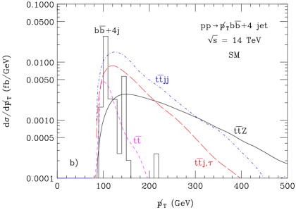
Figure 2: a) The differential cross sections at the LHC as a function of $p_{T}(Z)$ for ${\ell^{\prime}}^{+}{\ell^{\prime}}^{-}\ell\nu b\bar{b}jj$ final states. Shown are the SM predictions for $t\bar{t}Z$ production, for several non-standard $ttZ$ couplings, and for various backgrounds. Only one coupling at a time is allowed to deviate from its SM value. b) The differential cross sections as a function of the missing transverse momentum for $p\hbox to0.0pt{\hss/}_{T}b\bar{b}+4$j production at the LHC. Shown are the SM predictions for $t\bar{t}Z$ production and for various backgrounds.

The $Z$ boson transverse momentum distribution for the trilepton final state is shown in Fig. 2a for the SM signal and backgrounds, as well as for the signal with several non-standard $ttZ$ couplings. Only one coupling at a time is allowed to deviate from its SM prediction. The backgrounds are each more than one order of magnitude smaller than the SM signal. Note that varying $F^{Z}_{1V,A}$ leads mostly to a cross section normalization change, hardly affecting the shape of the $p_{T}(Z)$ distribution.

For the $p\hbox to0.0pt{\hss/}_{T}b\bar{b}+4j$ [10] final state at least 3 jets with $p_{T}>50$ GeV and $p\hbox to0.0pt{\hss/}_{T}>5~{}{\rm GeV}^{1/2}\sqrt{\sum p_{T}}$ are required. The largest backgrounds for this final state come from $t\bar{t}$ and $b\bar{b}+4j$ production where one or several jets are badly mismeasured, from $pp\to t\bar{t}jj$ with $t\bar{t}\to\ell^{\pm}\nu_{\ell}b\bar{b}jj$ and the charged lepton being missed, and from $t\bar{t}j$ production, where one top decays hadronically, $t\to Wb\to bjj$, and the other via $t\to Wb\to\tau\nu_{\tau}b$ with the $\tau$-lepton decaying hadronically, $\tau\to h\nu_{\tau}$.

In Fig. 2b we show the missing transverse momentum distributions of the SM $t\bar{t}Z\to p\hbox to0.0pt{\hss/}_{T}b\bar{b}+4j$ signal (solid curve) and various backgrounds. The most important backgrounds are $t\bar{t}jj$ and $t\bar{t}j$ production. However, the missing transverse momentum distribution from these processes falls considerably faster than that of the signal, and for $p\hbox to0.0pt{\hss/}_{T}>300$ GeV, the SM signal dominates.

5 Sensitivity Bounds for $ttV$ Couplings: LHC and ILC

The shape and normalization changes of the photon or $Z$-boson transverse momentum distribution can be used to derive sensitivity bounds on the anomalous $tt\gamma$ and $ttZ$ couplings. For $t\bar{t}Z$ production with $Z\to{\ell}^{+}{\ell}^{-}$, the distribution of the ${\ell}^{+}{\ell}^{-}$ opening angle in the transverse plane, $\Delta\Phi({\ell}{\ell})$, provides additional information [6]. In the following we assume a normalization uncertainty of the SM cross section of $\Delta{\cal N}=30\%$.

Even for a modest integrated luminosity of 30 fb^-1, it will be possible to measure the $tt\gamma$ vector and axial vector couplings, and the dipole form factors, with a precision of typically $20\%$ and $35\%$, respectively. For 300 fb^-1, the limits improve to $4-7\%$ for $F^{\gamma}_{1V,A}$ and to about $20\%$ for $F^{\gamma}_{2V,A}$.

To extract bounds on the $ttZ$ couplings, we perform a simultaneous fit to the $p_{T}(Z)$ and the $\Delta\Phi({\ell^{\prime}}{\ell^{\prime}})$ distributions for the trilepton and dilepton final states, and to the $p\hbox to0.0pt{\hss/}_{T}$ distribution for the $p\hbox to0.0pt{\hss/}_{T}b\bar{b}+4j$ final state. For an integrated luminosity of 300 fb^-1, it will be possible to measure the $ttZ$ axial vector coupling with a precision of $10-12\%$, and $F^{Z}_{2V,A}$ with a precision of $40\%$. At the SLHC, assuming an integrated luminosity of 3000 fb^-1, these bounds can be improved by factors of about 1.6 ($F^{Z}_{2V,A}$) and 3 ($F^{Z}_{1A}$). The bounds which can be achieved for $F^{Z}_{1V}$ are much weaker than those projected for $F^{Z}_{1A}$. As mentioned in Sec. 4, the $p_{T}(Z)$ distributions for the SM and for $F^{Z}_{1V,A}=-F^{Z,SM}_{1V,A}$ are almost degenerate. This is also the case for the $\Delta\Phi({\ell^{\prime}}{\ell^{\prime}})$ distribution. In a fit to these two distributions, therefore, an area centered at $\Delta F^{Z}_{1V,A}=-2F^{Z,SM}_{1V,A}$ remains which cannot be excluded, even at the SLHC. For $F^{Z}_{1V}$, the two regions merge, resulting in rather poor limits.

It is instructive to compare the bounds for anomalous $ttV$ couplings achievable at the LHC with those projected for the ILC. The most complete study of $t\bar{t}$ production at the ILC for general $ttV$ ($V=\gamma,\,Z$) couplings so far is that of Ref. [5]. Note that only one coupling at a time is allowed to deviate from its SM value in Ref. [5]. Comparing the projected LHC and ILC sensitivity bounds, one finds [11] that, even if the SLHC operates first, and the $p\hbox to0.0pt{\hss/}_{T}b\bar{b}+4j$ final state is taken into account, a linear collider will still be able to significantly improve the $ttZ$ anomalous coupling limits, with the possible exception of $\widetilde{F}^{Z}_{1A}$. The ILC will also be able to considerably strengthen the bounds on $\widetilde{F}^{\gamma}_{1A}$ and $\widetilde{F}^{\gamma}_{2A}$. It should be noted, however, that this picture could change once correlations between different non-standard $ttZ$ couplings, and between $tt\gamma$ and $ttZ$ couplings, are taken into account. Unfortunately, so far no realistic studies for $e^{+}e^{-}\to t\bar{t}$ which include these correlations have been performed.

6 Model Implications

Many models of new physics predict anomalous $ttZ$ couplings. Examples are top-seesaw models [12] and Little Higgs models [13], which predict an up-type quark singlet $T$ which mixes with the top quark. This changes coupling of the left-handed top quark to the $Z$-boson:

$$\Delta F^{Z}_{1V}=-\Delta F^{Z}_{1A}=F^{Z,SM}_{1A}\sin^{2}\theta_{L}\,$$ (2)

where $\theta_{L}$ is the $T-t$ mixing angle.

It is straightforward to derive bounds for $\sin^{2}\theta_{L}$ from the general limits on $F^{Z}_{1V,A}$ outlined in Sec. 5. With 300 fb^-1, $\sin^{2}\theta_{L}$ can be restricted to

$$\sin^{2}\theta_{L}<0.084~{}(0.16)\qquad{\rm at~{}68.3\%~{}(95\%)~{}CL}.$$ (3)

At the SLHC it will be possible to improve these bounds by about a factor 2.8.

In the $SU(5)/SO(5)$ Littlest Higgs model with T-parity [14], $\sin^{2}\theta_{L}$ is related to the mass of the heavy top quark partner, $T$, the $tTh$ coupling ($h$ is the Higgs boson), $\lambda_{T}$, and the SM Higgs vacuum expectation value, $v\approx 246$ GeV, by

$$\sin^{2}\theta_{L}={\lambda_{T}^{2}v^{2}\over 2m^{2}_{T}}.$$ (4)

In this model, the bounds on $\sin^{2}\theta_{L}$ can be converted into limits on $m_{T}/\lambda_{T}$. For 300 fb^-1 one finds [15]

$${m_{T}\over\lambda_{T}}>600~{}(430)~{}{\rm GeV}\qquad{\rm at~{}68.3\%~{}(95\%)~{}CL}.$$ (5)

Since the LHC should be able to discover a $T$ quark with a mass of $m_{T}\leq 2$ TeV [16], a measurement of $F^{Z}_{1A}$ can provide valuable information on $\lambda_{T}$.

7 Conclusions

The LHC will be able to perform first tests of the $ttV$ couplings. Already with an integrated luminosity of 30 fb^-1, one can probe the $tt\gamma$ couplings with a precision of about $10-35\%$ per experiment. With higher integrated luminosities one will be able to reach the few percent region. The LHC will also be able to probe the $ttZ$ couplings, albeit not with the same level of precision. However, a measurement of $F^{Z}_{1A}$ will constrain the parameter space of models with an extra up-type singlet quark, such as Little Higgs models. The ILC will be able to further improve our knowledge of the $ttV$ couplings, in particular in the $ttZ$ case.

References

- [1] F. Abe et al. (CDF Collaboration), Phys. Rev. Lett. 74, 2626 (1995).
- [2] S. Abachi et al. (DØ Collaboration), Phys. Rev. Lett. 74, 2632 (1995).
- [3] D. Chakraborty, J. Konigsberg and D. L. Rainwater, Ann. Rev. Nucl. Part. Sci. 53, 301 (2003); S. Eidelman et al. [Particle Data Group], Phys. Lett. B 592, 1 (2004).
- [4] F. Larios, M. A. Perez and C. P. Yuan, Phys. Lett. B457, 334 (1999); M. Frigeni and R. Rattazzi, Phys. Lett. B269, 412 (1991).
- [5] T. Abe et al. (American Linear Collider Working Group Collaboration), arXiv:hep-ex/0106057.
- [6] U. Baur, A. Juste, L. H. Orr and D. Rainwater, Phys. Rev. D71, 054013 (2005).
- [7] W. Hollik et al., Nucl. Phys. B551, 3 (1999) [Erratum-ibid. B557, 407 (1999)].
- [8] ATLAS TDR, report CERN/LHCC/99-15 (1999); Ph. Schwemling, ATLAS note SN-ATLAS-2003-034.
- [9] G. Altarelli, L. Conti and V. Lubicz, Phys. Lett. B502, 125 (2001) and references therein.
- [10] U. Baur, A. Juste, L. H. Orr and D. Rainwater, Phys. Rev. D73, 034016 (2006).
- [11] A. Juste et al., arXiv:hep-ph/0601112.
- [12] B. A. Dobrescu and C. T. Hill, Phys. Rev. Lett. 81, 2634 (1998).
- [13] For a recent review and more references see M. Schmaltz and D. Tucker-Smith, Ann. Rev. Nucl. Part. Sci. 55, 229 (2005).
- [14] J. Hubisz, P. Meade, A. Noble and M. Perelstein, JHEP 0601, 135 (2006).
- [15] C. F. Berger, M. Perelstein and F. Petriello, arXiv:hep-ph/0512053.
- [16] G. Azuelos et al., Eur. Phys. J. C 39S2, 13 (2005).