The BFKL Pomeron Calculus: Probabilistic
Interpretation and High Energy Amplitude.

Abstract:

In this paper we continue to pursue a goal of finding the effective theory for high energy interaction in QCD based on the colour dipole approach, for which the BFKL Pomeron Calculus gives a low energy limit. The two key problems, that we consider are the following: the probabilistic interpretation of the BFKL Pomeron Calculus and the possible scenario for the asymptotic behaviour of the scattering amplitude at high energy in QCD. In this paper we show that the generating functional approach is equivalent to the BFKL Pomeron Calculus and leads to a clear interpretation of this calculus as an alternative description of the system of interacting colourless dipoles.

We calculated the two BFKL Pomerons into one BFKL Pomeron vertex directly in the dipole approach and show that this merging can be described as the decay of two dipoles into four dipoles in the dipole approach. This result means the JIMWLK approach can give us all needed vertices for the BFKL Pomeron calculus and, therefore, they together give the selfconsistent and complete theoretical approach to high energy scattering in QCD.

In this paper, we developed the semi-classical approach to the functional evolution equation for the generating functional. Using this method we found the solution in the entire kinematic region starting from low energies for the simplified case of the toy model in which we assume that interaction of dipoles does not depend on their sizes. In the general case we find the asymptotic solution at ultra high energies as well as the first correction to this solution.

We considered the semi-classical approach to the BFKL Pomeron Calculus and recovered the Mueller-Shoshi band for the kinematic region where we can trust the linear BFKL equations. The solution for the scattering amplitude deeply in the saturation region was found and discussed.

1 Introduction

The simplest approach that we can propose for high energy interaction is based [1, 2] on the BFKL Pomeron [3] and reggeon-like diagram technique for the BFKL Pomeron interactions [4, 5, 6, 7]. This technique , which is a generalization of Gribov Reggeon Calculus [8], can be written in the elegant form of the functional integral (see Ref. [5] and the next section); and it is a challenge to solve this theory in QCD finding the high energy asymptotic behaviour. However, even this simple approach has not been solved during three decades of attempts by the high energy community. This failure stimulates a search for deeper understanding of physics which is behind the BFKL Pomeron Calculus. On the other hand, it has been known for three decades that Gribov Reggeon Calculus has intrinsic difficulties [9] that are related to the overlapping of Pomerons. Indeed, due to this overlapping we have no hope that the Gribov Reggeon Calculus could be correct in describing the ultra high energy asymptotic behaviour of the amplitude. The way out of these difficulties we see in searching for a new approach which will coincide with the BFKL Pomeron Calculus at high, but not very high, energies (our correspondence principle) but it will be different in the region of ultra high energies. In a spirit of the parton approach we believe that this effective theory should be based on the interaction of ‘wee’ partons. We consider, as an important step in this direction, the observation that has been made at the end of the Reggeon era [10, 11, 12], that the Reggeon Calculus can be reduced to a Markov process [13] for the probability of finding a given number of Pomerons at fixed rapidity $Y$. Such an interpretation, if it would be reasonable in QCD, can be useful, since it allows us to use powerful methods of statistical physics in our search for the solution.

The logic and scheme of our approach looks as follows. The first step is the Leading Log (1/x) Approximation (LLA) of perturbative QCD in which we sum all contributions of the order of $\left(\alpha_{S}\,\ln(1/x)\right)^{n}$. In the LLA we consider such high energies that

$$\alpha_{S}\,\ln(1/x)\,\,\approx\,\,1\,;\,\,\,\,\,\,\mbox{while}\,\,\,\,\,\,\,\alpha_{S}\,\,\ll\,\,1$$ (1.1)

It is well known that the LLA approach generates the BFKL Pomeron (see Ref. [3] and the next section) which leads to the power-like increase of the scattering amplitude ($A\,\propto\,\frac{1}{x^{\omega(n=0,\nu=0)}}$ with
$\omega(n=0,\nu=0)\,\,\propto\,\alpha_{S}$).

The second step is the BFKL Pomeron Calculus in which we sum all contributions of the order of

$$\left(\frac{\bar{\alpha}_{S}^{2}}{N^{2}_{c}}\,\frac{1}{x^{\omega(n=0,\nu=0)}}\right)^{n}\,\,\,\,\,\,\mbox{therefore}\,\,\,\,\,\,\,\frac{\bar{\alpha}_{S}^{2}}{N^{2}_{c}}\,\frac{1}{x^{\omega(n=0,\nu=0)}}\,\,\approx\,\,1$$ (1.2)

where $\bar{\alpha}_{S}\,\,=\,\,\alpha_{S}N_{c}/\pi$.

The structure of this approach as well as its parameter has been understood before QCD [14] and was confirmed in QCD (see Refs. [1, 2, 4, 5, 6, 7, 15, 16]). This calculus extends the region of energies from $\ln(1/x)\approx\,1/\bar{\alpha}_{S}$ of LLA to $\ln(1/x)\approx\,(1/\bar{\alpha}_{S})\ln(N^{2}_{c}/\bar{\alpha}_{S})$. The BFKL Pomeron Calculus describes correctly the scattering process in the region of energy:

$$\frac{1}{\bar{\alpha}_{S}}\,\,\ln\left(\frac{N^{2}_{c}}{\bar{\alpha}_{S}}\right)\,\,\ll\,\,ln\frac{1}{x}\,\,\ll\,\,\,\frac{1}{\bar{\alpha}_{S}^{2}}$$ (1.3)

For higher energies the corrections of the order of $\left(\bar{\alpha}_{S}^{2}\,\ln(1/x)\right)^{n}$ should be taken into account making all calculations very complicated.

Our credo is that we will be able to describe the high energy processes outside of the region of Eq. (1.3), if we could find an effective theory which describes the BFKL Pomeron calculus in the kinematic region given by Eq. (1.3), but based on the microscopic degrees of freedom and not on the BFKL Pomeron. In so doing, we hope that we can avoid all intrinsic difficulties of the BFKL Pomeron calculus and build an approximation that will be in an agreement with all general theorems like the Froissart bounds and so on. Solving this theory, we can create a basis for moving forward considering all corrections to this theory due to higher orders in $\bar{\alpha}_{S}$ contributions, running QCD coupling and so on.

The goal of this paper is to consider two main problems: the probabilistic interpretation of the BFKL Pomeron Calculus based on the idea that colour dipoles are the correct degrees of freedom at high energy QCD [17]; and the possible solution for scattering amplitude at high energy. We believe that colourless dipoles and their interaction will lead to a future theory at high energies which will have the BFKL Pomeron Calculus as the low energy limit (see Eq. (1.3)) and which will allow us to avoid all difficulties of dealing with BFKL Pomerons at ultra high energies.

Colourless dipoles play two different roles in our approach. First, they are partons (‘wee’ partons) for the BFKL Pomeron. This role is not related to the large $N_{c}$ approximation and, in principle, we can always speak about probability to find a definite number of dipoles instead of defining the probability to find a number of the BFKL Pomerons. The second role of the colour dipoles is that at high energies we can interpret the vertices of Pomeron merging and splitting in terms of probability for two dipoles annihilate in one dipole and of probability for decay of one dipole into two ones. It was shown in Ref. [17] that $P\rightarrow 2P$ splitting can be described as the process of the dipole decay into two dipoles. However, the relation between the Pomeron merging ($2P\rightarrow P$) and the process of annihilation of two dipoles into one dipole is not so obvious and it will be discussed here.

This paper is a next step in our programme of searching the simplest but correct approach to high energy scattering in QCD in which we continue the line of thinking presented in Refs. [18, 19, 20, 21]. The outline of the paper looks as follows.

In the next section we will discuss the BFKL Pomeron Calculus in the elegant form of the functional integral, suggested by M. Braun about five years ago [5]. We will show that the intensive recent work on this subject [22, 23, 20] confirms the BFKL Pomeron Calculus in spite of the fact that these attempts were based on slightly different but not more general assumptions.

In the third section the general approach based on the generating functional will be discussed. The set of equations for the amplitude of $n$-dipole interaction with the target will be obtained and the interrelations between vertices of the Pomeron interactions and the microscopic dipole processes will be considered. It will be shown that the generating functional approach is equivalent to the BFKL Pomeron Calculus in the kinematic region of Eq. (1.3) and leads to a clear interpretation of the BFKL Pomeron Calculus as an alternative description of the system of interacting colorless dipoles.

The Fourth section is devoted to the probabilistic interpretation of the BFKL Pomeron Calculus and, in particular, the process of merging of two Pomerons in one. We calculate the vertex of this merging directly in the dipole approach and show that it is related to the process of two dipole decay into four dipoles. We discuss the toy model which simplify the QCD interaction and allows us to see the main properties of high energy amplitude. In particular, we are going to discuss the solution of the equations for the asymptotic behaviour of the scattering amplitude at high energies. We find the solution for the generating functional in the entire phase space of both variables: rapidity $Y$ and the variable $u$ which is a conjugate variable to the number of dipoles.

In the fifth section we discuss the solution to the generating functional at high energies. We confirm the analysis of Ref. [21] and find the asymptotic solution suggested there. However, we study in more details the mechanism of approaching the ultra high energy limit for the scattering amplitude.

In conclusion we are going to compare our approach with other approaches on the market.

2 The BFKL Pomeron Calculus

2.1 The general structure of the BFKL Pomeron calculus.

We start with a general structure of the BFKL Pomeron calculus in QCD. The BFKL Pomeron exchange can be written in the form (see Fig. 1-1)

$$A(\mbox{{Fig.~{}\ref{bfklcal}}-1})\,\,=\,\,\,V_{u}\bigotimes G_{P}(r_{1},r_{2};b|Y_{1}-Y_{2})\bigotimes V_{d}\,\,\propto\,\,\frac{\bar{\alpha}_{S}^{2}}{N^{2}_{c}}\,\exp\left(\omega(n=0,\nu=0)\,(Y_{1}-Y_{2})\right)$$ (2.4)

with $\omega(n=0,\nu=0)\,\propto\,\bar{\alpha}_{S}$ and $\bigotimes$ denotes the all needed integrations. $Y_{1}-Y_{2}=\ln(1/x)$. To understand the main parameters of the BFKL Pomeron calculus, it is enough to compare the contribution of the first ‘fan’ diagram of Fig. 1-2 with the one BFKL Pomeron exchange. This diagram has the following contribution

$$A(\mbox{{Fig.~{}\ref{bfklcal}}-2}) = \int^{Y_{1}}_{Y_{2}}\,dY^{\prime}\,V_{u}\,\bigotimes\,G_{P}(r_{1},r^{\prime};b|Y_{1}-Y^{\prime})\,\bigotimes\,\Gamma(1\to 2)G^{2}_{P}(\{r^{\prime}\},r_{2};b|Y^{\prime}-Y_{2})\bigotimes V^{2}_{d}\$$

$$\propto \frac{V_{u}\,V^{2}_{d}\,\Gamma(1\to 2)}{\omega(n=0,\nu=0)}\,\exp\left(2\,\omega(n=0,\nu=0)\,Y\right)\,\,\propto\,\left(\frac{\bar{\alpha}_{S}^{2}}{N^{2}_{c}}\right)^{2}\,\,\exp\left(2\,\omega(n=0,\nu=0)\,Y\right)$$

where $Y=Y_{1}-Y_{2}$; $R_{1}$ and $r_{2}$ are the sizes of the projectile and target dipoles while $\{r^{\prime}\}$ denotes all dipole variables in Pomeron splitting and/or merging.

One can see that the ratio of this two diagrams is proportional to $\frac{\bar{\alpha}_{S}^{2}}{N^{2}_{c}}\,\exp\left(\omega(n=0,\nu=0)(Y_{1}-Y_{2})\right)$ which is the parameter given by Eq. (1.2). When this ration is about 1 we need to calculate all diagrams with the Pomeron exchange and their interactions (see Fig. 1-a - Fig. 1-f ). All vertices, that are shown in Fig. 1, has been calculated in Refs. [4, 5] and they have the following order in $\bar{\alpha}_{S}$ :

$$\omega(n=0,\nu=o)\,\,\,\propto\,\,\,\bar{\alpha}_{S}\,\,;\,\,\,\,\,\,\,\,\Gamma(1\to 2)\,\,\,\propto\,\,\,\frac{\bar{\alpha}_{S}^{2}}{N_{c}}\,\,;\,\,\,\,\,\,\,\,\,\Gamma(2\to 1)\,\,\,\propto\,\,\,\frac{\bar{\alpha}_{S}^{2}}{N_{c}}\,\,;$$

$$\Gamma(2\to 2)\,\,\,\propto\,\,\,\frac{\bar{\alpha}_{S}}{N^{2}_{c}}\,\,;\Gamma(2\to 3)\,\,\,\propto\,\,\,\frac{\bar{\alpha}_{S}^{2}}{N^{2}_{c}}\,\,;V_{u}\,\,\propto\,\,\,\frac{\bar{\alpha}_{S}}{N_{c}}\,\,;V_{d}\,\,\propto\,\,\,\frac{\bar{\alpha}_{S}}{N_{c}}\,;$$ (2.6)

Using Eq. (2.6) we can easily estimate the contributions of all diagrams in Fig. 1. Namely,

$$A(\mbox{{Fig.~{}\ref{bfklcal}}-3}) \,\,\,\propto\,\,\, V_{u}\,V_{d}\,\,\frac{\Gamma(1\to 2)\,\Gamma(2-1)}{\omega^{2}(n=0,\nu=0)}\exp\left(2\omega(n=0,\nu=0)(Y_{1}-Y_{2})\right)$$

$$\propto \,\,\,\left(\frac{\bar{\alpha}_{S}^{2}}{N^{2}_{c}}\,\exp\left(\omega(n=0,\nu=0)(Y_{1}-Y_{2})\right)\right)^{2}\,\,=\,\,L^{2}\left(Y\right)\,\,;$$ (2.7)

$$A(\mbox{{Fig.~{}\ref{bfklcal}}-4}) \,\,\,\propto\,\,\, V_{u}\,V^{2}_{d}\,\,\frac{\Gamma(1\to 2)}{\omega(n=0,\nu=0)}\,\Gamma(2\to 2)\,(Y_{1}-Y_{2})\,\exp\left(2\omega(n=0,\nu=0)(Y_{1}-Y_{2})\right)$$ (2.8)

$$\propto \,\,\,\frac{\bar{\alpha}_{S}}{N^{2}_{c}}\,\left(Y_{1}-Y_{2}\right)\,\left(\frac{\bar{\alpha}_{S}^{2}}{N^{2}_{c}}\,\exp\left(\omega(n=0,\nu=0)(Y_{1}-Y_{2})\right)\right)^{2}\,\,=\,\,\frac{\bar{\alpha}_{S}}{N^{2}_{c}}\,Y\,L^{2}\left(Y\right)\,\,;$$

$$A(\mbox{{Fig.~{}\ref{bfklcal}}-5}) \,\,\,\propto\,\,\, V_{u}\,V^{3}_{d}\,\,\frac{\Gamma(1\to 2)\,\,\Gamma(2\to 3)}{2\,\omega^{2}(n=0,\nu=0)}\,\,\exp\left(3\omega(n=0,\nu=0)(Y_{1}-Y_{2})\right))$$ (2.9)

$$\propto \,\,\,\frac{1}{N^{2}_{c}}\,\left(\frac{\bar{\alpha}_{S}^{2}}{N^{2}_{c}}\,\exp\left(\omega(n=0,\nu=0)(Y_{1}-Y_{2})\right)\right)^{3}\,\,=\,\,\frac{1}{N^{2}_{c}}\,\,L^{3}\left(Y\right);$$

$$A(\mbox{{Fig.~{}\ref{bfklcal}}-6)} \,\,\,\propto\,\,\, V_{u}\,V_{d}\,\,\frac{\Gamma(1\to 2)\,\Gamma(2\to 1)}{\omega^{2}(n=0,\nu=0)}\,\Gamma(2\to 2)\,(Y_{1}-Y_{2})\,\exp\left(2\omega(n=0,\nu=0)(Y_{1}-Y_{2})\right))$$ (2.10)

$$\propto \,\,\,\frac{\bar{\alpha}_{S}}{N^{2}_{c}}(Y_{1}-Y_{2})\,\,\,\left(\frac{\bar{\alpha}_{S}^{2}}{N^{2}_{c}}\,\exp\left(\omega(n=0,\nu=0)(Y_{1}-Y_{2})\right)\right)^{2}\,\,=\,\,\frac{\bar{\alpha}_{S}}{N^{2}_{c}}\,Y\,\,L^{2}\left(Y\right);$$

with $L\left(Y\right)\,\,=\,\,\left(\bar{\alpha}_{S}^{2}/N^{2}_{c}\right)\,\,\exp\left(\omega(n=0,\nu=0)\,Y\right)$.

As we have mentioned in the introduction the BFKL calculus sums all diagrams at so high energy that parameter $L(Y)$ is of the order of 1 (see Eq. (1.2)). In this kinematic region we need to take into account the diagrams of Fig. 1 -1 , Fig. 1-2 and Fig. 1-3 (see Eq. (2.4),Eq. (2.1) and Eq. (2.7)). Indeed, diagrams of Fig. 1-4 and Fig. 1-6 ( see Eq. (2.8) and Eq. (2.10)) are small since $(\bar{\alpha}_{S}^{2}/N^{2}_{c})\,Y\,\,\ll\,\,1/N^{2}_{c}\,\,\ll\,\,1$ in the kinematic region of Eq. (1.3), while the diagrams of Fig. 1-5 (see Eq. (2.9)) is small at $L\left(Y\right)\approx 1$.

The first conclusion that we can derive from this analysis that in the kinematic region where $L\left(Y\right)\,\,\approx\,\,1$ we need to take into account all diagrams with $\Gamma(1\to 2)$ and $\Gamma(2\to 1)$ vertices while the diagrams with $\Gamma(2\to 2)$ and $\Gamma(2\to 3)$ vertices give small, negligible contributions.

However, if $L\left(Y\right)\,\,\propto\,\,N_{c}$ one can see from Eq. (2.4) - Eq. (2.10) that all diagrams give so essential contributions that we have to take them into account. For what follows it is interesting to notice that the vertex $\Gamma(2\to 2)\,\propto\,\,\bar{\alpha}_{S}^{4}/N^{2}_{c}$ can be neglected even at such large values of $L\left(Y\right)$.

Finally, we can conclude that the first step of our approach can be summing of the diagrams with $\Gamma(1\to 2)$ and $\Gamma(2\to 1)$ vertices. Namely, this approach we discuss below in details.

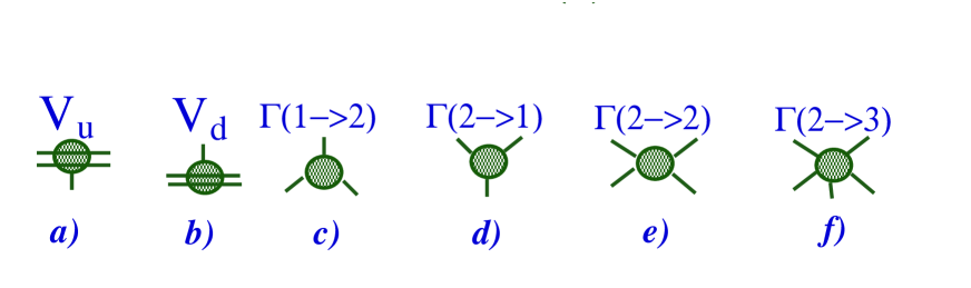
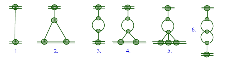
Figure 1: The BFKL Pomeron interactions and the examples of the diagrams of the BFKL Pomeron calculus in QCD. The solid line describes the Pomeron exchange while the double line stands for the dipole.

However, we would like to stress that we need to make an additional assumption inherent for the BFKL Pomeron calculus: the multi-gluon states in $t$-channel of the scattering amplitude lead to smaller contribution at high energies than the exchange of the appropriate number of the BFKL Pomerons (see more in Ref.[21]). The real argument, supporting this assumption, stems from the numerous attempts to find the intercept of these states, larger than the one for the multi-Pomeron exchanges [25] that failed.

2.2 The path integral formulation of the BFKL calculus

The main ingredient of the BFKL Pomeron calculus is the Green function of the BFKL Pomeron describing the propagation of a pair of gluons from rapidity $Y^{\prime}$ and points $x^{\prime}_{1}$ and $x^{\prime}_{2}$ to rapidity $Y$ and points $x_{1}$ and $x_{2}$ Since the Pomeron does not carry colour in $t$-channel we can treat initial and final coordinates as coordinates of quark and antiquark in a colourless dipole. This Green function is well known[26] and has a form:

$$G(x_{1},x_{2};Y|x^{\prime}_{1},x^{\prime}_{2};Y^{\prime})\,\,=\,\,\Theta(Y-Y^{\prime})\times$$ (2.11)

$$\times\,\sum^{\infty}_{n=-\infty}\,\int\,d\nu\,\,d^{2}x_{0}\,e^{\omega(n,\nu)(Y-Y^{\prime})}\,\lambda(n,\nu)\,E(x_{1},x_{2};x_{0}|\nu)\,E^{*}(x^{\prime}_{1},x^{\prime}_{2};x_{0}|\nu)$$

where vertices $E$ are given by

$$E(x_{1},x_{2};x_{0}|\nu)\,=\,\left(\frac{x_{12}}{x_{10}\,x_{20}}\right)^{h}\,\left(\frac{x^{*}_{12}}{x^{*}_{10}\,x^{*}_{20}}\right)^{\tilde{h}}$$ (2.12)

where $x_{ik}=x_{i}-x_{k}$, $x_{i}=x_{i,x}+ix_{i,y}$ ,$x^{*}_{i}=x_{i,x}+ix_{i,y}$ ; $h=(1-n)/2+i\nu$ and $\tilde{h}=1-h^{*}$. The energy levels $\omega(n,\nu)$ are the BFKL eigen values

$$\omega(n,\nu)\,=\,\bar{\alpha}_{S}\left(\psi(1)-Re{\,\psi\left(\frac{|n|+1}{2}+i\nu\right)}\right)$$ (2.13)

where $\psi(z)=d\ln\Gamma(z)/dz$ and $\Gamma(z)$ is the Euler gamma function. Finally

$$\lambda(n,\nu)\,=\frac{1}{[(n+1)^{2}+4\nu^{2}][(n-1)^{2}+4\nu^{2}]}$$ (2.14)

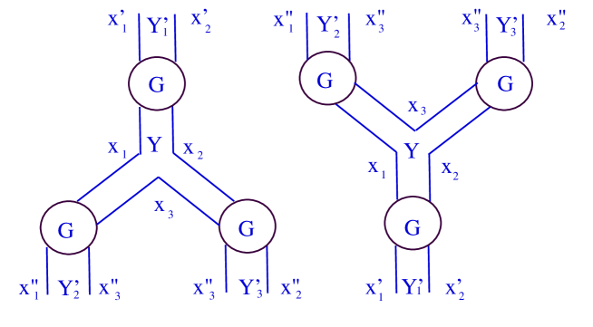
Figure 2: The graphic form of the triple Pomeron vertex in the coordinate representation.

The interaction between Pomerons is depicted in Fig. 2 and described by the triple Pomeron vertex which can be written in the coordinate representation [5] for the following process: two gluons with coordinates $x^{\prime}_{1}$ and $x^{\prime}_{2}$ at rapidity $Y^{\prime}_{1}$ decay into two gluons pairs with coordinates $x^{\prime\prime}_{1}$ and $x^{\prime\prime}_{3}$ at rapidity $Y^{\prime}_{2}$ and $x^{\prime\prime}_{2}$ and $x^{\prime\prime}_{3}$ at rapidity $Y^{\prime}_{3}$ due to the Pomeron splitting at rapidity $Y$. It looks as

$$2\frac{\pi\,\bar{\alpha}^{2}_{S}}{N_{c}}\,\int\,\frac{d^{2}x_{1}\,d^{2}\,x_{2}\,d^{2}x_{3}}{x^{2}_{12}\,x^{2}_{23}\,x^{2}_{13}}\,\left(G(x^{\prime}_{1},x^{\prime}_{2};Y^{\prime}_{1}|x_{1},x_{2};Y)\,\,L^{\!\!\!\!\!\!\!\leftarrow}_{1,2}\right)\cdot$$ (2.15)

$$G(x_{1},x_{3};Y|x^{\prime\prime}_{1},x^{\prime\prime}_{3};Y^{\prime}_{2})\,G(x_{3},x_{2};Y|x^{\prime\prime}_{3},x^{\prime\prime}_{2};Y^{\prime}_{3})$$

where

$$L^{\!\!\!\!\!\!\!\leftarrow}_{1,2}\,\,=\,\,r^{4}_{12}\,p^{2}_{1}\,p^{2}_{2}\,\,\,\mbox{with}\,\,p^{2}\,=\,-\,\nabla^{2}$$ (2.16)

and arrow shows the direction of action of the operator $L$. For the inverse process of merging of two Pomerons into one we have

$$2\frac{\pi\,\bar{\alpha}^{2}_{S}}{N_{c}}\,\int\,\frac{d^{2}x_{1}\,d^{2}\,x_{2}\,d^{2}x_{3}}{x^{2}_{12}\,x^{2}_{23}\,x^{2}_{13}}\,G(x^{\prime\prime}_{1},x^{\prime\prime}_{3};Y^{\prime}_{1}|x_{1},x_{3};Y)\,G(x^{\prime\prime}_{3},x^{\prime\prime}_{2};Y^{\prime}_{2}|x_{3},x_{2};Y)\,\cdot$$

$$\left(L^{\!\!\!\!\!\rightarrow}_{1,2}\,G(x_{1},x_{2};Y|x^{\prime}_{1},x^{\prime}_{2};Y^{\prime}_{1})\right)$$ (2.17)

The theory with the interaction given by Eq. (2.15) and Eq. (2.17) can be written through the functional integral [5]

$$Z[\Phi,\Phi^{+}]\,\,=\,\,\int\,\,D\Phi\,D\Phi^{+}\,e^{S}\,\,\,\mbox{with}\,S\,=\,S_{0}\,+\,S_{I}\,+\,S_{E}$$ (2.18)

where $S_{0}$ describes free Pomerons, $S_{I}$ corresponds to their mutual interaction while $S_{E}$ relates to the interaction with the external sources (target and projectile). From Eq. (2.15) and Eq. (2.17) it is clear that

$$S_{0}\,=\,\int\,dY\,dY^{\prime}\,d^{2}x_{1}\,d^{2}x_{2}\,d^{2}x^{\prime}_{1}\,d^{2}x^{\prime}_{2}\,\Phi^{+}(x_{1},x_{2};Y)\,G^{-1}(x_{1},x_{2};Y|x^{\prime}_{1},x^{\prime}_{2};Y^{\prime})\,\Phi(x^{\prime}_{1},x^{\prime}_{2};Y^{\prime})$$ (2.19)

$$S_{I}\,=\,\frac{2\,\pi\bar{\alpha}_{S}^{2}}{N_{c}}\,\int\,dY\,\int\,\frac{d^{2}x_{1}\,d^{2}x_{2}\,d^{2}x_{3}}{x^{2}_{12}\,x^{2}_{23}\,x^{2}_{13}}\,\cdot\{\left(L^{\!\!\!\!\!\rightarrow}_{1,2}\Phi(x_{1},x_{2};Y)\,\right)\,\cdot\,\Phi^{+}(x_{1},x_{3};Y)\,\Phi^{+}(x_{3},x_{2};Y)\,\,+\,\,h.c.\}$$ (2.20)

For $S_{E}$ we have local interaction both in rapidity and in coordinates, namely,

$$S_{E}\,=\,-\,\int\,dY\,d^{2}x_{1}\,d^{2}x_{2}\,\{\Phi(x_{1},x_{2};Y)\,\tau_{pr}(x_{1},x_{2};Y)\,\,+\,\,\Phi^{+}(x_{1},x_{2};Y)\,\tau_{tar}(x_{1},x_{2};Y)\}$$ (2.21)

where $\tau_{pr}$ ($\tau_{tar}$) stands for the projectile and target, respectively. The form of functions $\tau$ depend on the non-perturbative input in our problem and for the case of nucleus target they are written in Ref. [5].

For the case of the projectile being a dipole that scatters off a nucleus the scattering amplitude has the form

$$T(x_{1},y_{1};Y)\,\,\equiv T^{(1)}(x_{1},y_{1};Y)\,\,=\,\,-\,\frac{4\,\pi^{2}\,\bar{\alpha}_{S}}{N_{c}}\,\frac{\int\,\,D\Phi\,D\Phi^{+}\,\Phi(x_{1},y_{1};Y)\,e^{S[\Phi,\Phi^{+}]}}{\int\,\,D\Phi\,D\Phi^{+}\,\,e^{S[\Phi,\Phi^{+}]}|_{S_{E}=0}}$$ (2.22)

where extra $\alpha_{S}$ comes from our normalization and where we neglect term with $\tau_{pr}$ in Eq. (2.21).

Generally, for the amplitude of interaction of $n$ dipoles at rapidity $Y$ we can write the following expression

$$T^{(n)}(x_{1},y_{1},\dots x_{n},y_{n};Y)\,\,=\,\,(-1)^{n}\left(\,\frac{4\,\pi^{2}\,\bar{\alpha}_{S}}{N_{c}}\,\right)^{n}\,\frac{\int\,\,D\Phi\,D\Phi^{+}\,\prod^{n}_{i=1}\Phi(x_{i},y_{i};Y)\,\,e^{S[\Phi,\Phi^{+}]}}{\int\,\,D\Phi\,D\Phi^{+}\,\,e^{S[\Phi,\Phi^{+}]}|_{S_{E}=0}}$$ (2.23)

The extra factor $(-1)^{n}$ stems from the fact that in $S_{E}$ the source for a projectile as well as for a target, has an extra minus sign.

It is useful to introduce the Green function of the BFKL Pomeron that includes the Pomeron loops. This function has the form

$$G\left(x_{1},y_{1};Y|x_{2},y_{2};Y^{\prime}\right)\,\,=\,\,\frac{\int\,\,D\Phi\,D\Phi^{+}\,\Phi^{+}(x_{1},y_{1};Y)\,\Phi(x_{2},y_{2};Y^{\prime})\,\,e^{S[\Phi,\Phi^{+}]}}{\int\,\,D\Phi\,D\Phi^{+}\,\,e^{S[\Phi,\Phi^{+}]}|_{S_{E}=0}}$$ (2.24)

For further presentation we need some properties of the BFKL Green function [26]:

1. Generally,

$$G^{-1}(x_{1},x_{2};Y|x^{\prime}_{1},x^{\prime}_{2};Y^{\prime})\,\,\,=\,p^{2}_{1}\,p^{2}_{2}\,\left(\frac{\partial}{\partial Y}+H\right)\,\,=\,\,\left(\frac{\partial}{\partial Y}+H^{+}\right)\,p^{2}_{1}\,p^{2}_{2};$$ (2.25)

$$Hf(x_{1},x_{2};Y)\,\,=\,\,\frac{\bar{\alpha}_{S}}{2\pi}\,\int\,\frac{d^{2}x_{3}\,x^{2}_{12}}{x^{2}_{23}\,x^{2}_{13}}\,\left(f(x_{1},x_{2};Y)\,-\,f(x_{1},x_{3};Y)\,-\,f(x_{3},x_{2};Y)\right);$$ (2.26)

2. The initial Green function ($G_{0}$) is equal to

$$G_{0}(x_{1},x_{2};Y|x^{\prime}_{1},x^{\prime}_{2};Y)\,\,=\,\,\pi^{2}\,\ln\frac{x^{2}_{1,1^{\prime}}\,x^{2}_{2,2^{\prime}}}{x^{2}_{1,2^{\prime}}\,x^{2}_{1^{\prime},2}}\,\ln\frac{x^{2}_{1,1^{\prime}}\,x^{2}_{2,2^{\prime}}}{x^{2}_{1,2}\,x^{2}_{1^{\prime},2^{\prime}}}$$ (2.27)

This form of $G_{0}$ has been discussed in Ref.[26]. In appendix A we demonstrate that this expression for $G_{0}(x_{1},x_{2};Y|x^{\prime}_{1},x^{\prime}_{2};Y)$ stems from $\omega=\omega(n=0,\nu)$ term in sum of Eq. (2.11). Only this term is essential at high energies since all other terms lead to decreasing with energy contributions.

3. It should be stressed that

$$\nabla^{2}_{1}\,\nabla^{2}_{2}\,G_{0}(x_{1},x_{2};Y|x^{\prime}_{1},x^{\prime}_{2};Y)\,\, =$$

$$\,\,(2\,\pi)^{4}\,\,\left(\delta^{(2)}(x_{1}-x^{\prime}_{1})\,\delta^{(2)}(x_{2}-x^{\prime}_{2})\,+\,\delta^{(2)}(x_{1}-x^{\prime}_{2})\,\delta^{(2)}(x_{2}-x^{\prime}_{1})\,\right)$$

4. In sum of Eq. (2.11) only the term with $n=0$ is essential for high energy asymptotic behaviour since all $\omega(n,\nu)$ with $n\geq 1$ are negative and, therefore, lead to contributions that decrease with energy. Taking into account only the first term one can see that $G$ is the eigen function of operator $L_{13}$, namely

$$L_{12}\,G(x_{1},x_{2};Y|x^{\prime}_{1},x^{\prime}_{2};Y^{\prime})\,\,=\,\,\frac{1}{\lambda(0,\nu)}\,G(x_{1},x_{2};Y|x^{\prime}_{1},x^{\prime}_{2};Y^{\prime})\,\,\approx\,\,G(x_{1},x_{2};Y|x^{\prime}_{1},x^{\prime}_{2};Y^{\prime});$$ (2.29)

The last equation holds only approximately in the region where $\nu\,\ll\,1$, but this is the most interesting region which is responsible for high energy asymptotic behaviour of the scattering amplitude.

2.3 The chain of equations for the multi-dipole amplitudes.

Using Eq. (2.18) and Eq. (2.22) we can easily obtain the chain equation for multi-dipole amplitude $T^{(n)}$ noticing that every dipole interacts only with one Pomeron (see Eq. (2.22)).

These equations follow from the fact that a change of variables does not alter the value of functional integral of Eq. (2.18). In particular, $Z[\Phi,\Phi^{+}]\,=\,Z[\Phi,\Phi^{\prime+}]$(see Eq. (2.18) ) where $\Phi^{\prime+}\,=\,\Phi^{+}\,+\,\epsilon(x,y)$ with small function $\epsilon(x,y)$. Therefore,

$$\int\,D\,\Phi\,D\,\Phi^{+}\,e^{S[\Phi\,,\Phi^{+}]}\,\,=\,\,\int\,D\,\Phi\,D\,\Phi^{\prime+}\,e^{S[\Phi\,,\Phi^{\prime+}]}$$ (2.30)

Substituting $\Phi^{\prime+}\,=\,\Phi^{+}\,+\,\epsilon(x,y)$ and expanding this equation to first order in $\epsilon$, we find

$$0\,=\,\int\,D\,\Phi\,D\,\Phi^{+}\,e^{S[\Phi\,,\Phi^{+}]}\,\times$$ (2.31)

$$[\,\int\,dY\,dY^{\prime}\,d^{2}x_{1}\,d^{2}x_{2}\,d^{2}x^{\prime}_{1}\,d^{2}x^{\prime}_{2}\,\epsilon(x_{1},x_{2};Y)\,G^{-1}(x_{1},x_{2};Y|x^{\prime}_{1},x^{\prime}_{2};Y^{\prime})\,\Phi(x^{\prime}_{1},x^{\prime}_{2};Y^{\prime})$$

$$+\frac{2\,\pi\bar{\alpha}_{S}^{2}}{N_{c}}\,\int\,dY\,\int\,\frac{d^{2}x_{1}\,d^{2}x_{2}\,d^{2}x_{3}}{x^{2}_{12}\,x^{2}_{23}\,x^{2}_{13}}\,\cdot\{\left(\epsilon(x_{1},x_{2};Y)L^{\!\!\!\!\!\leftarrow}_{1,2}\,\right)\,\cdot\,\Phi(x_{1},x_{3};Y)\,\Phi(x_{3},x_{2};Y)+$$

$$2\left(L^{\!\!\!\!\!\rightarrow}_{1,2}\Phi(x_{1},x_{2};Y)\,\right)\,\cdot\,\epsilon(x_{1},x_{3};Y)\,\Phi^{+}(x_{3},x_{2};Y)\}-\,\int\,dY\,d^{2}x_{1}\,d^{2}x_{2}\,\epsilon(x_{1},x_{2};Y)\,\tau_{tar}(x_{1},x_{2};Y)]$$

We redefine the integration variables in the third term as follows

$$2\left(L^{\!\!\!\!\!\rightarrow}_{1,2}\Phi(x_{1},x_{2};Y)\,\right)\,\cdot\,\epsilon(x_{1},x_{3};Y)\,\Phi^{+}(x_{3},x_{2};Y)\longrightarrow 2\left(L^{\!\!\!\!\!\rightarrow}_{1,3}\Phi(x_{1},x_{3};Y)\,\right)\,\cdot\,\epsilon(x_{1},x_{2};Y)\,\Phi^{+}(x_{2},x_{3};Y)$$

Using the expression for the Hamiltonian Eq. 2.25 and the Casimir operator Eq. 2.16 we define a new variation parameter $\epsilon(x_{1},x_{2};Y)p^{2}_{1}\,p^{2}_{2}$. In terms of this variation parameter Eq. 2.31 reads as

$$0\,=\,\int\,D\,\Phi\,D\,\Phi^{+}\,e^{S[\Phi\,,\Phi^{+}]}\,\times$$ (2.32)

$$[\,\int\,dY\,d^{2}x_{1}\,d^{2}x_{2}\;\;\epsilon(x_{1},x_{2};Y)p^{2}_{1}p^{2}_{2}\left(\frac{\partial}{\partial Y}+H\right)\Phi(x_{1},x_{2};Y)$$

$$+\frac{2\,\pi\bar{\alpha}_{S}^{2}}{N_{c}}\,\int\,dY\,\int\,\frac{d^{2}x_{1}\,d^{2}x_{2}\,d^{2}x_{3}}{x^{2}_{12}\,x^{2}_{23}\,x^{2}_{13}}\,\cdot\{\left(\epsilon(x_{1},x_{2};Y)p^{2}_{1}p^{2}_{2}\right)\,\cdot\,\Phi(x_{1},x_{3};Y)\,\Phi(x_{3},x_{2};Y)+$$

$$2\left(L^{\!\!\!\!\!\rightarrow}_{1,3}\Phi(x_{1},x_{3};Y)\,\right)\,\cdot\,\epsilon(x_{1},x_{2};Y)\,\frac{p^{2}_{1}p^{2}_{2}}{p^{2}_{1}p^{2}_{2}}\,\Phi^{+}(x_{3},x_{2};Y)\}-\,\int\,dY\,d^{2}x_{1}\,d^{2}x_{2}\,\epsilon(x_{1},x_{2};Y)\frac{p^{2}_{1}p^{2}_{2}}{p^{2}_{1}p^{2}_{2}}\,\tau_{tar}(x_{1},x_{2};Y)]$$

We denote the new variation parameter by $\tilde{\epsilon}(x_{1},x_{2};Y)=p^{2}_{1}p^{2}_{2}\epsilon(x_{1},x_{2};Y)$ and use the property of the initial Green function Eq. 2.2 to rewrite $\frac{1}{p^{2}_{1}p^{2}_{2}}$ in terms of $G_{0}$ as follows

$$\frac{1}{p^{2}_{1}p^{2}_{2}}\tilde{\epsilon}(x_{1},x_{2};Y)\,\,=\,\,\frac{1}{(2\pi)^{4}}\int G_{0}(x_{1},x_{2};Y|x^{\prime}_{1},x^{\prime}_{2};Y)\tilde{\epsilon}(x^{\prime}_{1},x^{\prime}_{2};Y)d^{2}x^{\prime}_{1}d^{2}x^{\prime}_{2}$$ (2.33)

Thus, Eq. 2.32 can be written as

$$0\,=\,\int\,D\,\Phi\,D\,\Phi^{+}\,e^{S[\Phi\,,\Phi^{+}]}\,\times$$ (2.34)

$$[\,\int\,dY\,d^{2}x_{1}\,d^{2}x_{2}\;\;\tilde{\epsilon}(x_{1},x_{2};Y)\left(\frac{\partial}{\partial Y}+H\right)\Phi(x_{1},x_{2};Y)$$

$$+\frac{2\,\pi\bar{\alpha}_{S}^{2}}{N_{c}}\,\int\,dY\,\int\,\frac{d^{2}x_{1}\,d^{2}x_{2}\,d^{2}x_{3}}{x^{2}_{12}\,x^{2}_{23}\,x^{2}_{13}}\,\cdot\{\tilde{\epsilon}(x_{1},x_{2};Y)\,\,\Phi(x_{1},x_{3};Y)\,\Phi(x_{3},x_{2};Y)+$$

$$2\left(L^{\!\!\!\!\!\rightarrow}_{1,3}\Phi(x_{1},x_{3};Y)\,\right)\,\cdot\,\left\{\frac{1}{(2\pi)^{4}}\int G_{0}(x_{1},x_{2};Y|x^{\prime}_{1},x^{\prime}_{2};Y)\tilde{\epsilon}(x^{\prime}_{1},x^{\prime}_{2};Y)d^{2}x^{\prime}_{1}d^{2}x^{\prime}_{2}\right\}\,\Phi^{+}(x_{3},x_{2};Y)\}$$

$$-\,\int\,dY\,d^{2}x_{1}\,d^{2}x_{2}\,\left\{\frac{1}{(2\pi)^{4}}\int G_{0}(x_{1},x_{2};Y|x^{\prime}_{1},x^{\prime}_{2};Y)\tilde{\epsilon}(x^{\prime}_{1},x^{\prime}_{2};Y)d^{2}x^{\prime}_{1}d^{2}x^{\prime}_{2}\right\}\,\tau_{tar}(x_{1},x_{2};Y)]$$

Noting that the r.h.s. of Eq. (2.34) should vanish for any possible variation $\tilde{\epsilon}(x_{1},x_{2};Y)$ we obtain

$$0\,=\,\int\,D\,\Phi\,D\,\Phi^{+}\,e^{S[\Phi\,,\Phi^{+}]}\,\times[\left(\frac{\partial}{\partial Y}+H\right)\Phi(x_{1},x_{2};Y)$$ (2.35)

$$+\frac{2\,\pi\bar{\alpha}_{S}^{2}}{N_{c}}\,\,\int\,\frac{x^{2}_{12}\,d^{2}x_{3}}{x^{2}_{23}\,x^{2}_{13}}\Phi(x_{1},x_{3};Y)\,\Phi(x_{3},x_{2};Y)+$$

$$+\frac{2\,\pi\bar{\alpha}_{S}^{2}}{N_{c}}\,\frac{2}{(2\pi)^{4}}\,\int\,\frac{\,d^{2}x^{\prime}_{1}\,d^{2}x^{\prime}_{2}\,d^{2}x_{3}}{x^{2}_{1^{\prime}2^{\prime}}x^{2}_{2^{\prime}3}\,x^{2}_{1^{\prime}3}}\left(x^{4}_{1^{\prime}3}\;p^{2}_{1^{\prime}}p^{2}_{3}\Phi(x_{1}^{\prime},x_{3};Y)\,\right)G_{0}(x^{\prime}_{1},x^{\prime}_{2};Y|x_{1},x_{2};Y)\,\Phi^{+}(x_{3},x^{\prime}_{2};Y)\}$$

$$-\frac{1}{(2\pi)^{4}}\,\int d^{2}x^{\prime}_{1}d^{2}x^{\prime}_{2}G_{0}(x^{\prime}_{1},x^{\prime}_{2};Y|x_{1},x_{2};Y)\,\tau_{tar}(x^{\prime}_{1},x^{\prime}_{2};Y)]$$

where in the third and last terms we interchanged $(x^{\prime}_{1},x^{\prime}_{2})\leftrightarrow(x_{1},x_{2})$. We notice that the third and last terms are independent of rapidity and can be absorbed in the initial condition. It is obvious for the last term which represents the target source. To show this for the third term we use the property of the Casimir operator at high energies ($n=0\;,\;\nu=0$)

$$L^{\!\!\!\!\!\rightarrow}_{1,3}\Phi(x_{1},x_{3};Y)\simeq\Phi(x_{1},x_{3};Y)$$

and the definition of the Green function(see Eq. 2.24). We see that the third term results into the product of two initial Green functions which are independent of rapidity.

Now we can use the definition of the amplitude defined in Eq. 2.22 and Eq. 2.23 to rewrite Eq. 2.35 in a simple form

$$\frac{\partial T^{(1)}(x_{1},x_{2};Y)}{\partial Y}\,\,=\,\,\frac{\bar{\alpha}_{S}}{2\,\pi}\,\int\,d^{2}\,z\,K(x_{1},x_{2};z)\,$$ (2.36)

$$\left(T^{(1)}(x_{1},z;Y)\,+\,T^{(1)}(z,x_{2};Y)\,-\,T^{(1)}(x_{1},x_{2};Y)\,-\,T^{(2)}(Y;x_{1},z;z,x_{2};Y)\right)$$

where kernel $K(x,y|z)$ is defined as

$$K(x,y|z)\,\,=\,\,\frac{(x-y)^{2}}{(x-z)^{2}\,(z-y)^{2}}$$ (2.37)

and the Hamiltonian is given by Eq. 2.26.

This equation has a very simple meaning that is clear from Fig. 3.

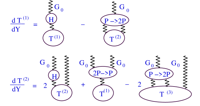
Figure 3: The graphic form of equations for the multi dipole amplitude.

Starting from equation

$$\int\,D\,\Phi\,D\,\Phi^{+}\,\Phi(Y;x_{4},x_{5})\,\,e^{S[\Phi\,,\Phi^{+}]}\,\,=\,\,\int\,D\,\Phi\,D\,\Phi^{\prime+}\,\Phi(Y;x_{4},x_{5})\,\,e^{S[\Phi\,,\Phi^{\prime+}]}$$ (2.38)

we obtain the equation for the amplitude $T^{(2)}$, namely,

$$\frac{\partial T^{(2)}(x_{1},x_{2};x_{3},x_{4};Y)}{\partial Y}\,\,=\,\,\frac{\bar{\alpha}_{S}}{2\,\pi}\int\,d^{2}\,z\,K(x_{1},x_{2}|z)\,$$ (2.39)

$$\left(T^{(2)}(x_{1},z;x_{3},x_{4};Y)\,+\,T^{(2)}(z,x_{2};x_{3},x_{4};Y)\,-\,\,T^{(2)}(x_{1},x_{2};x_{3},x_{4};Y)\,-\right.$$

$$\left.-\,T^{(3)}(x_{1},z;z,x_{2};x_{3},x_{4};Y)\right)\,+$$

$$+\,2{\alpha}^{2}_{S}\frac{\bar{\alpha}_{S}}{2\,\pi}\int\,d^{2}\,x^{\prime}\,d^{2}\,x^{\prime\prime}\,\Gamma_{2\to 1}(x_{1},x_{2};x_{3},x_{4}|x^{\prime},x^{\prime\prime})\,\nabla^{2}_{x^{\prime}}\nabla^{2}_{x^{\prime\prime}}T^{(1)}(x^{\prime},x^{\prime\prime};Y);$$

where function $\Gamma_{2\to 1}$ is equal to

$$\Gamma_{2\to 1}(x_{1},y_{1};x_{2},y_{2}|x,y)\,\,=\int\,d^{2}zK(x,y;z)\,\,G_{0}(x_{1},y_{1}|x,z)\,G_{0}(x_{1},y_{1}|z,y)$$ (2.40)

Deriving Eq. (2.36) and Eq. (2.39) we use Eq. (2.27) and Eq. (2.2) as well as normalization condition (see Eq. (2.22)) for the scattering amplitude. These two equations are the same as in Ref. [27]. This shows that in the papers [22, 27], actually, the same approach as the BFKL Pomeron Calculus has been developed (much later, of course), in spite of the fact that authors think that they are doing something more general.

Assuming that $T^{(2)}=T^{(1)}\,T^{(1)}$ we obtain the Balitsky-Kovchegov equation [28, 29]. We can do this only if we can argue why the Pomeron splitting is more important than the Pomeron merging. For example, this assumption is reasonable for scattering of the dipole with the nucleus target. Generally speaking, the splitting and merging have the same order in $\alpha_{S}$ ( see Eq. (2.15) and Eq. (2.17). In Eq. (2.36) and Eq. (2.39) these two processes look like having a different order of magnitude in $\alpha_{S}$ but this fact does not interrelate with any physics and reflects only our normalization. However, we will see that for a probabilistic interpretation the correct normalization is very important.

3 Generating functional and probabilistic interpretation

3.1 Statistical physics analogy: Langevin equation and directed percolation.

The functional of Eq. (2.18) is reminiscent of the partition function of statistical mechanics. Indeed, the partition function has a general form

$$Z[H]\,\,=\,\,e^{-\frac{1}{kT}\,F[H]}\,\,=\,\,\int d{\bf s}\,e^{-\frac{1}{kT}\,\int\,dx\left({\cal H}(s)\,-H\,s(x)\right)}$$ (3.41)

where $F[H]$ is the Helmholtz free energy. As an example, Eq. (3.41) is written for the system of spins with the energy density ${\cal H}(s)$ in the external magnetic field $H$. The integration is over all possible configurations of spins in the system.

Comparing Eq. (3.41) and Eq. (2.18) one can see that Eq. (2.18) describes a statistical system with $kT=1$ and with $F[-\tau_{tr}]=-S$. The form of $S_{E}$ suggests that $H=-\tau_{tr}$ plays a role of the external field.

Eq. (2.18) on the lattice looks as follows

$$Z[\Phi,\Phi^{+}]\,\,=\,\,\int\,\prod_{i}\,D\,\Phi_{i}(x_{i},y_{i};Y_{i})\,D\,\Phi^{+}_{i}(x_{i},y_{i};Y_{i})\,e^{S[\Phi_{i},\Phi^{+}_{i}]}$$ (3.42)

We can linearize the action using the Stratonovich transformation [30] but first we simplify the expression for action $S$ introducing a new field $\Phi^{+^{\prime}}(x_{1},x_{2};Y)\,=\,p^{2}_{1}\,p^{2}_{2}\Phi^{+}(x_{1},x_{2};Y)$ and using Eq. (2.25) , Eq. (2.29) and Eq. (2.33). In new notation the action has the form

$$S_{0}\,=\,\int\,dY\,dY^{\prime}\,d^{2}xd^{2}y\,d^{2}x^{\prime}\,d^{2}y^{\prime}\,\Phi^{+^{\prime}}(x,y;Y)\,\left(\frac{\partial}{\partial Y^{\prime}}\,+\,H\,\right)\,\Phi(x^{\prime},y^{\prime};Y^{\prime})$$ (3.43)

$$S_{I}\,=\,\,\frac{2\,\pi\bar{\alpha}_{S}^{2}}{N_{c}}\,\,\left(\int\,dY\,d^{2}x\,d^{2}yd^{2}z\,K(x,y|z)\,\Phi^{+^{\prime}}(x,y;Y)\,\Phi(x,z;Y)\,\Phi(z,y;Y)\,\,+\,\,\right.$$ (3.44)

$$\left.\frac{1}{(2\pi)^{8}}\,\,\prod^{3}_{i=1}\,d^{2}\,x_{i}\,d^{2}\,y_{i}\,\frac{\Gamma_{2\to 1}(x_{1},y_{1};,x_{2},y_{2}|x_{3},y_{3})}{(x_{3}-y_{3})^{4}}\,\Phi^{+^{\prime}}(x_{1},y_{1};Y)\,\Phi^{+^{\prime}}(x_{2},y_{2};Y)\,\Phi(x_{3},y_{3};Y)\right)$$

while $S_{E}$ has the form

$$S_{E}\,\,=\,\,-\,\,\frac{1}{(2\pi)^{4}}\,\,\int\,dY\,\,d^{2}\,x\,d^{2}\,y\,d^{2}\,x^{\prime}\,d^{2}\,y^{\prime}\,\,\Phi^{+^{\prime}}(x,y;Y)\,G_{0}(x,y|x^{\prime},y^{\prime})\,\tau(x^{\prime},y^{\prime};Y)$$ (3.45)

We demonstrate the idea of the statistical interpretation of our theory using the simplified version, so called toy model, in which we assume that there is no dependence of the interaction on the coordinate of dipoles (see Ref. [17] for details). The action of this model is

$$S\,\,=\,\,\int\,dY\,\left(\Phi^{+}(Y)\,\left(\frac{d}{dY}\,-\,\Delta\right)\Phi(Y)\,+\right.$$ (3.46)

$$\left.\,G_{3P}\left(\Phi^{+}(Y)\,\Phi^{2}(Y)\,+\,\Phi(Y)\,(\Phi^{+})^{2}(Y)\right)-\Phi^{+}(Y)\,\tau_{tr}(Y)\delta(Y-Y_{0})\right)$$

where $G_{3P}$ is the toy-model vertex that describes the one Pomeron to two Pomerons transition.

Using the Stratonovich transformation we can linearize the action given by Eq. (3.46), namely,

$$\exp\left(G_{3P}\,\Delta Y\,\Phi_{i}\,(\Phi^{+}_{i})^{2}\,\right)\,\sim\,\,\int\,\,d\eta_{i}\,\exp\left(\,-\frac{1}{2}\eta^{2}_{i}\,-\,\Phi^{+}_{i}\,\sqrt{2\,G_{3P}\,\Phi_{i}\,\Delta Y}\,\eta_{i}\right)$$ (3.47)

Substituting Eq. (3.47) into Eq. (3.42) and integrating explicitly over $\Phi^{+}_{i}$ we obtain

$$Z\,\,\propto\,\int\,\prod_{i}\,D\,\Phi_{i}\,D\,\eta_{i}\,e^{-\frac{1}{2}\sum_{i}\int\,dY\,\eta^{2}_{i}}\,\delta\left(d\,\Phi_{i}\-\,\,\Delta\Phi_{i}\,+\,\,G_{3P}\Phi^{2}_{i}-\,\,\sqrt{2\,G_{3P}\,\Phi_{i}\,dY}\,\eta_{i}\right)$$ (3.48)

The $\delta$-function means that the only $\Phi$ which satisfy to the following (Langevin) equation

$$d\,\Phi(Y)\,\,=\,\,\Delta\,\,\Phi(Y)\,\,-\,\,G_{3P}\,\Phi^{2}\,d\,Y\,\,+\,\,\sqrt{2\,G_{3P}\,\Phi}\,dW(Y)$$ (3.49)

(where $W(Y)$ is a Wiener process [13]) contribute to the functional integral. Eq. (3.49) is actually the Langevin equation for directed percolation (see Ref. [31] for details) which can be re-written in the form

$$\frac{\partial\,\,\Phi(Y)}{\partial Y}\,\,\,=\,\,\Delta\,\Phi(Y)\,\,\,-\,\,\,G_{3P}\,\,\Phi^{2}(Y)\,\,+\,\,\zeta(Y)$$ (3.50)

where $\zeta$ is a density ($\Phi$) dependent Gaussian noise field [31, 13, 32, 33, 22, 23], which is defined as

$$<|\zeta(Y)|>\,\,=\,\,0\,;\,\,\,\,\,\,\,\,<|\zeta(Y)\,\,\zeta(Y^{\prime})|>\,\,=\,\,2\,G_{3P}\,\Phi(Y)\,\delta(Y-Y^{\prime})\,\,.$$ (3.51)

The general functional of Eq. (3.42), we believe, can be reduced to Eq. (3.50). However, we found a way how to do this only for Eq. (3.42) only with addinional sipsimplificationse assume (i) that Eq. (2.29) has the form

$$L_{12}\,\,G\left(x_{1},x_{2};Y|x^{\prime}_{1},x^{\prime}_{2};Y^{\prime}\right)\,\,=\,\,G\left(x_{1},x_{2};Y|x^{\prime}_{1},x^{\prime}_{2};Y^{\prime}\right)$$ (3.52)

or, in other words, we consider $\Lambda(n,\nu)\,\,=\,\,\Lambda(n=0,\nu)\,\,=\,\,\Lambda(n=0,\nu=0)$ (see Eq. (2.14)) , which gives the leading contribution for the BFKL calculus; and (ii) that

$$\frac{x_{1}\,+\,x_{2}}{2}\,\,\gg\,\,x_{1}\,-\,x_{2}\,\,;$$ (3.53)

Indeed, we expect that the typical size of the dipoles will be of the order of $1/Q_{s}(x)$ ($Q_{s}(x)$ is the satrusaturatione) while the typical impact parameter of the scattering dipole should be much larger (at least of the order of the size of the hadron).

Using these two assumptions we can rewrite the functional integral in the form of Eq. (2.18) but with action $S_{I}$ that can be written as follows

$$S_{I}\,\,=\,\,\frac{2\,\pi\,\bar{\alpha}_{S}^{2}}{N_{c}}\,\int\,d\,Y\,\,\int\,\frac{d^{2}x_{1}\,d^{2}x_{2}\,d^{2}x_{3}}{x^{2}_{12}\,x^{2}_{23}\,x^{2}_{13}}\,\cdot\,\,\{\,\Phi(x_{1},x_{2};Y)\,\cdot\,\Phi^{+}(x_{1},x_{3};Y)\,\Phi^{+}(x_{3},x_{2};Y)\,\,+\,\,h.c.\}$$ (3.54)

and Eq. (2.25) reads as

$$G^{-1}(x_{1},x_{2};Y|x^{\prime}_{1},x^{\prime}_{2};Y^{\prime})\,\,\,=\,p^{2}_{1}\,p^{2}_{2}\,\left(\frac{\partial}{\partial Y}+H\right)\,\,=\,\,\frac{1}{x^{4}_{12}}\left(\frac{\partial}{\partial Y}+H\right)$$ (3.55)

Collecting Eq. (3.54), Eq. (3.55) and Eq. (2.26) one can see that the action has a simple form

$$S_{0}\,+\,S_{I}\,\, = \,\,\int\,\frac{d^{2}\,x_{1}\,d^{2}\,x_{2}}{x^{4}_{12}}\,\,\Phi^{+}\left(x_{1},x_{2};Y\right)\,\,\frac{\partial\Phi\left(x_{1},x_{2};Y\right)}{\partial\,Y}\,\,+\,\,$$

$$+ \,\,\int\,d\,Y\,\,\int\,\frac{d^{2}x_{1}\,d^{2}x_{2}\,d^{2}x_{3}}{x^{2}_{12}\,x^{2}_{23}\,x^{2}_{13}}\,\,\left(\frac{\bar{\alpha}_{S}}{2\pi}\,\,\Phi^{+}\left(x_{1},x_{2};Y\right)\,\,\left\{\,\Phi\left(x_{1},x_{2};Y\right)\,\,-\,\,\Phi\left(x_{1},x_{3};Y\right)\,\,-\,\,\Phi\left(x_{3},x_{2};Y\right)\right\}\,\,\right.$$ (3.56)

$$+ \left.\,\,\frac{2\,\pi\,\bar{\alpha}_{S}^{2}}{N_{c}}\cdot\,\,\{\,\Phi(x_{1},x_{2};Y)\,\,\cdot\,\Phi^{+}(x_{1},x_{3};Y)\,\Phi^{+}(x_{3},x_{2};Y)\,\,+\,\,h.c.\}\,\right)\,.$$

Eq. (3.56) can be reduce to more elegant form using Eq. (3.53) and going toomentum representation, namely,

$$\Phi(x_{1},x_{2};Y)\,\,=\,\,x^{2}_{12}\,\int\,d^{2}\,k\,e^{i\,\vec{k}\cdot\vec{x}_{12}}\,\,\Phi\left(k,b;Y\right)$$ (3.57)

where $b\,=\,(x_{1}+x_{2})/2\,\,\rightarrow\,\,(x_{1}+x_{3})/2\,\,=\,\,(x_{2}+x_{3})/2$ (see Eq. (3.53)).

In terms of fields $\Phi\left(k,b;Y\right)$ and $\Phi^{+}\left(k,b;Y\right)$ the action looks as follows

$$S\,\,=\,\,S_{0}\,+\,S_{I}\,\,=\,\,\int\,d^{2}\,b\,d^{2}\,k\,\,\Phi^{+}\left(b,k;Y\right)\,\,$$ (3.58)

$$\left(\frac{\partial\Phi\left(b,k;Y\right)}{\partial\,Y}\,\,-\,\,\frac{\bar{\alpha}_{S}}{2\pi}\,\int\,d^{2}\,k^{\prime}\,K\left(k,k^{\prime}\right)\,\Phi\left(b,k^{\prime};Y\right)\,\,+\,\,\frac{2\,\pi\,\bar{\alpha}_{S}^{2}}{N_{c}}\cdot\left\{\,\Phi^{+}b,k;Y)\,\Phi^{+}(b,k;Y)\,\,\,+\,\,\,h.c.\right\}\,\right)$$

where $K\left(k,k^{\prime}\right)$ is the BFKL kernel in the momentum representation, namely,

$$\int\,d^{2}\,k^{\prime}\,\,K\left(k,k^{\prime}\right)\,\,\Phi\left(b,k^{\prime};Y\right)\,\,=\,\,\int\,d^{2}\,k^{\prime}\,\,\frac{\Phi\left(b,k^{\prime};Y\right)}{(k-k^{\prime})^{2}}\,\,-\,\,k^{2}\,\int\,d^{2}\,k^{\prime}\,\frac{\Phi\left(b,k;Y\right)}{(k-k^{\prime})^{2}\,(k^{\prime 2}\,+\,(k-k^{\prime})^{2})}$$ (3.59)

The action $S$ of Eq. (3.58) looks very similar to the action of the toy model (see Eq. (3.46)) and can be easily reduced to the Langevin equation for directed percolation

$$\frac{\partial\,\,\Phi\left(b,k;Y\right)}{\partial Y}\,\,\,=\,\,\frac{\bar{\alpha}_{S}}{2\pi}\,\int\,d^{2}\,k^{\prime}\,K\left(k,k^{\prime}\right)\,\Phi\left(b,k^{\prime};Y\right)\,\,\,-\,\,\,\frac{2\,\pi\,\bar{\alpha}_{S}^{2}}{N_{c}}\cdot\,\Phi(b,k;Y)\,\Phi^{(}b,k;Y)\,\,+\,\,\zeta(b,k;Y)$$ (3.60)

with

$$<|\zeta(b,k;Y)|>\,\,=\,\,0\,;\,\,\,\,\,\,\,\,\,\,\,<|\zeta(b,k;Y)\,\zeta(b^{\prime},k^{\prime};Y^{\prime})|>\,\,=\,\,\frac{4\,\pi\,\bar{\alpha}_{S}^{2}}{N_{c}}\cdot\Phi(b,k;Y)\,\delta^{(2)}(\vec{b}-\vec{b}^{\prime})\,\delta^{(2)}(\vec{k}-\vec{k}^{\prime})\,\delta\left(Y-Y^{\prime}\right)$$ (3.61)

Actually, we have shown (see Refs.L3,L4) and will discuss below that in QCD we expect a different form for the noise , namely,

$$<|\zeta(b,k;Y)|>\,\,=\,\,0\,;$$ (3.62)

$$\,\,\,\,\,\,\,\,\,\,\,<|\zeta(b,k;Y)\,\zeta(b^{\prime},k^{\prime};Y^{\prime})|>\,\,=\,\,\frac{4\,\pi\,\bar{\alpha}_{S}^{2}}{N_{c}}\cdot\Phi(b,k;Y)\,\left(1-\Phi(b,k;Y)\right)\delta^{(2)}(\vec{b}-\vec{b}^{\prime})\,\delta^{(2)}(\vec{k}-\vec{k}^{\prime})\,\delta\left(Y-Y^{\prime}\right)$$

which belongs to a diffrent universality class than Eq. (3.61) ([31, 34]) .

The Langevin equation is the one of many ways to describe a diffusion process and the condidereable progress has been achieved in this approach. (see Refs.[31, 32, 33, 22, 23, 36]).

However, we prefer a different way for description of the BFKL Pomeron interactions, which will also lead to diffusion equation: the so called generating functional approach. The advantage of the generating functional approach is its tansparent relation to the partonic wave function of the fast hadron (dipole) and, because of this, this approach can be a source of the new Monte Carlo approach for high energy scattering. In this approach we see in the most explicit way our main theoretical problem: the BFKL Pomeron calculus provides the amplitude that satisfies the $t$-channel unitarity while the $s$-channel unitarity is still a problem in the BFKL Pomeron calculus. However, the probabilistic interpretation in the framework of the generating functional leads to the correctly normalized partonic wave function which takes into account the main properties of the $s$-channel unitarity as well.

3.2 Generating functional: general approach

In this subsection we discuss the main equations of the BFKL Pomeron Calculus in the formalism of the generating functional, which we consider as the most appropriate technique for the probabilistic interpretation of this approach to high energy scattering in QCD.

To begin with let us write down the definition of the generating functional [17]

$$Z\left(Y\,-\,Y_{0};\,[u]\right)\,\,\equiv\,\,$$ (3.63)

$$\equiv\,\,\sum_{n=1}\,\int\,\,P_{n}\left(Y\,-\,Y_{0};\,x_{1},y_{1};\dots;x_{i},y_{i};\dots;x_{n},y_{n}\right)\,\,\prod^{n}_{i=1}\,u(x_{i},y_{i})\,d^{2}\,x_{i}\,d^{2}\,y_{i}$$

where $u(x_{i},y_{i})\equiv u_{i}$ is an arbitrary function of $x_{i}$ and $y_{i}$. The coordinates $(x_{i},y_{i})$ describe the colorless pair of gluons or a dipole. $P_{n}$ is a probability density to find $n$ dipoles with the size $x_{i}-y_{i}$, and with impact parameter $(x_{i}+y_{i})/2$. Directly from the physical meaning of $P_{n}$ and definition in Eq. (3.63) it follows that the functional (Eq. (3.63)) obeys the condition

$$Z\left(Y\,-\,Y_{0};\,[u=1]\right)\,\,=\,\,1\,.$$ (3.64)

The physical meaning of this equation is that the sum over all probabilities is equal to unity.

Introducing vertices for the dipole process: $1\to 2$ ($V_{1\to 2}(x,y\to x_{1},y_{1}+x_{2},y_{2})$), $2\to 1$ ($V_{2\to 1}(x_{1},y_{1}+x_{2},y_{2}\to x,y)$) and $2\to 3$ ($V_{2\to 3}(x_{1},y_{1}+x_{2},y_{2}\to x^{\prime}_{1},y^{\prime}_{1}+x^{\prime}_{2},y^{\prime}_{2}+x^{\prime}_{3},y^{\prime}_{3})$ we can write a typical birth-death equation in the form

$$\frac{\partial\,P_{n}(Y;\dots;x_{i},y_{i};\dots;x_{n},y_{n})}{\partial Y}\,\,\,=$$ (3.65)

$$= \,\,\sum_{i}\ V_{1\to 2}\bigotimes\left(P_{n-1}(Y;\dots;x_{i},y_{i};\dots;x_{n},y_{n})\,-\,P_{n}(Y;\dots;x_{i},y_{i};\dots;x_{n},y_{n})\right)$$ (3.66)

$$+ \,\,\sum_{i>k}V_{2\to 1}\,\bigotimes\,\left(P_{n+1}(Y;\dots;x_{k},y_{k};\dots;x_{i},y_{i};\dots:x_{n},y_{n})\,-\,P_{n}(Y;\dots;x_{i},y_{i};\dots;)\right)$$ (3.67)

$$+ \,\,\sum_{i>k}\,V_{2\to 3}\bigotimes\left(P_{n-1}(Y;x_{i},y_{i};\dots;x_{k},y_{k};\dots;x_{n},y_{n})\,-\,P_{n}(Y;x_{i},y_{i};\dots;x_{k},y_{k};\dots;x_{n},y_{n})\right)$$ (3.68)

Eq. (3.65) is the typical Markov’s chain and the fact that we have the correct normalized partonic wave function is written in Eq. (3.65) by introducing for each microscopic (dipole) process two terms (see Eq. (3.66),Eq. (3.67) and Eq. (3.68)): the emission of dipoles (positive birth term ) and their recombination (negative death term).

Multiplying this equation by the product $\prod^{n}_{i=1}\,u_{i}$ and integrating over all $x_{i}$ and $y_{i}$, we obtain the following linear equation for the generating functional:

$$\frac{\partial\,Z\,\left(Y-Y_{0};[\,u\,]\right)}{\partial\,Y}\,\,=\,\,\chi\,[\,u\,]\,\,Z\,\left(Y-Y_{0};[\,u\,]\right)$$ (3.69)

with

$$\chi[u]\,\, = \,\,\,\int\,d^{4}\,qd^{4}q_{1}\,d^{4}q_{2}\,\,\left(V_{1\,\rightarrow\,2}\left(q\to q_{1}+q_{2}\right)\,\left(-u(q)\,+\,u(q_{1})\,u(q_{2})\,\right)\,\frac{\delta}{\delta u(q)}\,-\right.$$ (3.71)

$$\left.-V_{2\,\rightarrow\,1}\left(q_{1}+q_{2}\to q\right)\,\left(u(q_{1})\,u(q_{2})\,-\,u(q)\right)\,\,\frac{1}{2}\,\frac{\delta^{2}}{\delta u(q_{1})\,\delta u(q_{2})}\right)\,;$$

Trying to make out presentation more transparent we omitted in Eq. (3.71) the term that corresponds to the $2\to 3$ transition (see Ref. [20] for full presentation). We also use notations $q_{i}$ for $(x_{i},y_{i})$ and $d^{4}q_{i}$ for $d^{2}x_{i}\,d^{2}\,y_{i}$ where $x_{i}$ and $y_{i}$ are positions of quark (antiquark) for the colourless dipole.

Eq. (3.69) is a typical diffusion equation or Fokker-Planck equation [13], with the diffusion coefficient which depends on $u$. This is the master equation of our approach, and the goal of this paper is to find the correspondence of this equation with the BFKL Pomeron Calculus and the asymptotic solution to this equation. In spite of the fact that this is a functional equation we intuitively feel that this equation could be useful since we can develop a direct method for its solution and, on the other hand, there exist many studies of such an equation in the literature ( see for example Ref. [13]) as well as some physical realizations in statistical physics. The intimate relation between the Fokker-Planck equation, and the high energy asymptotic was first pointed out by Weigert [32] in JIMWLK approach [37], and has been discussed in Refs. [33, 22, 23].

The scattering amplitude can be defined as a functional [29, 19]

$$N\left(Y;[\gamma_{i}]\right)\, = \,-\sum^{\infty}_{n=1}\int\gamma_{n}(x_{1},y_{1};\dots;x_{n},y_{n};Y_{0})\prod^{n}_{i=1}\frac{\delta}{\delta u_{i}}Z\left(Y,[u_{i}]\right)|_{u_{i}=1}\,d^{2}x_{i}\,d^{2}y_{i}$$

$$= \,-\,\sum^{\infty}_{n=1}(-1)^{n}\int\gamma_{n}(x_{1},y_{1};\dots;x_{n},y_{n};Y_{0})\,\,\rho(x_{1},y_{1};\dots;x_{n},y_{n};Y-Y_{0})$$

The physical meaning of functions $\gamma_{n}$ is the imaginary part of the amplitude of interaction of $n$-dipoles with the target at low energies. All these functions should be taken from the non-pertubative QCD input. However, in Refs. [18, 19, 20] it was shown that we can introduce the amplitude of interaction of $n$-dipoles ($\gamma_{n}(x_{1},y_{1};\dots;x_{n},y_{n};Y)$ at high energies (large values of rapidity $Y$) and Eq.  (3.63), Eq.  (3.69) and Eq.  (3.2) can be rewritten as a chain set of equation for $\gamma_{n}(x_{1},y_{1};\dots;x_{n},y_{n};Y)$. The equation has the form

$$\frac{\partial\,\gamma_{n}\left(q_{1}\dots,q_{n}\right)}{\partial\,Y}\,\,\,\,=2\,\sum_{i=1}^{n}\,\int\,d^{4}q^{\prime}\,d^{4}q\,V_{1\,\rightarrow\,2}(q_{i};\,q,\,q^{\prime})\,\gamma_{n}\left(\dots q^{\prime}\dots\right)\,$$

$$- \,\sum_{i=1}^{n}\,\int d^{4}q_{1}^{\prime}\,d^{4}q_{2}^{\prime}\,V_{1\,\rightarrow\,2}(q_{i};\,q_{1}^{\prime},\,q_{2}^{\prime})\,\gamma_{n}\left(\dots,q_{i}\dots\right)\,-\sum^{n-1}_{i=1}\int d^{4}q\,d^{4}q^{\prime}$$

$$V_{1\,\rightarrow\,2}(q_{i};\,q,\,q^{\prime})\,\gamma_{n+1}\left(\dots q\dots q^{\prime}\right)-\,\sum_{i>j}^{n}\,\int d^{4}\,q\,V_{2\,\rightarrow\,1}\left(q_{i},\,q_{j};\,q\right)$$

$$\cdot \gamma_{n-1}\left(q_{i}\dots q_{j}\dots q\right)\,+\,2\,\sum_{i=1}^{n}\int d^{4}q\,d^{4}q^{\prime}V_{2\rightarrow 1}\left(q,q_{i};q^{\prime}\right)\,\gamma_{n-1}\left(\dots q_{i}\dots q\right)\,+$$

$$+ \,\sum^{n}_{i,k,i>k}\,\int d^{4}q\,V_{2\rightarrow 1}\left(q_{i},q_{k};q\right)\,\gamma_{n}\left(\dots q_{i}\dots q_{k}\dots\right)$$

Comparing this equation for $\gamma_{1}\equiv T^{(1)}$ and $\gamma_{2}\equiv T^{(2)}$ one can see that

$$V_{1\to 2} = \frac{\bar{\alpha}_{S}}{2\,\pi}\Gamma_{1\to 2}\,\,=\,\,\frac{\bar{\alpha}_{S}}{2\,\pi}\,K\left(x,y;z\right)\,;$$ (3.74)

$$V_{2\to 1}\, = \,\,\frac{2\,\alpha^{2}_{S}}{\pi^{2}}\frac{\bar{\alpha}_{S}}{2\,\pi}\,\left(-\,\frac{\Gamma_{2\to 1}(x_{1},y_{1}+x_{2},y_{2}\to x,y)}{(x-y)^{4}}\,+\right.$$ (3.75)

$$+ \left.\,\,\int\,\frac{d^{2}x\,d^{2}y}{(x-y)^{4}}\,\Gamma_{2\to 1}(x_{1},y_{1}+x_{2},y_{2}\to x,y)\,\cdot\right.$$

$$\cdot \left.\left(\delta^{(2)}(x_{1}-x)\delta^{(2)}(y_{1}-y)\,+\,\delta^{(2)}(x_{2}-x)\delta^{(2)}(y_{2}-y)\right)\right)$$

with $\Gamma_{2\to 1}$ is given by Eq. (2.40).

3.3 A toy model: Pomeron interaction and probabilistic interpretation

In this section we consider the simple toy model in which the probabilities to find $n$-dipoles do not depend on the size of dipoles [17, 18, 20, 21]. In this model the master equation (3.69) has a simple form

$$\frac{\partial Z}{\partial Y}\,=\,-\Gamma(1\to 2)\,u(1-u)\,\frac{\partial Z}{\partial u}+\,\Gamma(2\to 1)\,u(1-u)\,\frac{\partial^{2}Z}{(\partial u)^{2}}$$ (3.76)

and this equation generates: the Pomeron splitting $G_{P\to 2P}=-\Gamma(1\to 2)$; Pomerons merging $G_{2P\to P}=\Gamma(2\to 1)$ and also the two Pomeron scattering $G_{2P\to 2P}\,\,=\,\,-\Gamma(2\to 1)$. It is easy to see that neglecting $u^{2}\partial^{2}Z/(\partial u)^{2}$ term in Eq. (3.76) we cannot provide a correct sign for Pomerons merging $G_{2P\to P}$.

The description given by Eq. (3.76) is equivalent to the path integral of Eq. (3.46). To see this we need to notice that the general solution of Eq. (3.76) has a form

$$Z(Y;u)\,\,=\,\,e^{H(u)\,(Y-Y_{0})}Z(Y_{0};u)$$ (3.77)

with operator $H$ defined as

$$H(u)\,\,=\,\,-\,\Gamma(1\to 2)\,u(1-u)\,\frac{\partial}{\partial u}+\,\Gamma(2\to 1)\,u(1-u)\,\frac{\partial^{2}}{(\partial u)^{2}}$$ (3.78)

and

$$Z(Y_{0};u)\,\,=\,\,e^{\tau_{tr}(u-1)}$$ (3.79)

Introducing operators of creation ($a^{+}$) and annihilation ($a$)

$$\hat{a}\,=\,\frac{\partial}{\partial u}\,;\,\,\,\,\,\,\,\,\,\,\hat{a}^{+}\,=\,u\,\,\,\mbox{that satisfy}\,\,[\hat{a},\hat{a}^{+}]=1\,\,\,\mbox{at fixed}\,\,Y$$ (3.80)

one can see that operator ${\cal H}$ has the form

$${\cal H}\,\,=\,\,-\,\Gamma(1\to 2)\,\hat{a}^{+}\,(1-\hat{a}^{+})\,\hat{a}\,\,+\,\,\Gamma(2\to 1)\,\hat{a}^{+}\,(1-\hat{a}^{+})\,\hat{a}^{2}$$ (3.81)

and the initial state at $Y=Y_{0}$ is defined as

$$|Y_{0}>\,\,=\,\,e^{\tau_{tr}(\hat{a}^{+}\,-\,1)}|0>$$ (3.82)

with the vacuum defined as $\hat{a}|0>=0$.

We need to discretize the development operator of Eq. (3.77) with ${\cal H}$ given by Eq. (3.81), namely,

$$e^{{\cal H}\,(Y-Y_{0})}=e^{{\cal H}\,\Delta Y}\,\dots\,e^{{\cal H}\,\Delta Y}=\,\prod^{N}_{j=1}\,\left(1\,+\,{\cal H}\,\Delta Y\right)$$ (3.83)

and introduce the coherent states [38] for a certain intermediate rapidity $Y_{j}=Y_{0}+j\Delta Y$ as

$$|\phi_{j}>\,\,=\,\,e^{\phi_{j}\,\hat{a}^{+}\,-\,\phi_{j}}\,|0>$$ (3.84)

where $\phi_{j}$ are arbitrary complex numbers. The initial state of Eq. (3.82) can be written as

$$|\phi_{0}(Y_{0})>\,\equiv|\tau_{tr}>.$$ (3.85)

The unit operator in terms of the coherent states can be expressed as

$$1\,=\,\left(\,\int\,\frac{d\phi_{j}d\phi_{j}^{*}}{\pi i}\,e^{-\phi_{j}\,\phi_{j}^{*}\,+\,\phi_{j}\,+\,\phi_{j}^{*}}\right)|\phi_{j}>\,<\phi_{j}|$$ (3.86)

We want to calculate matrix element of some operator $A$ between states of initial $Y_{0}$ and final $Y$ rapidity $<Y|A|Y_{0}>$. This can be written as

$$<Y|A|Y_{0}>=<Y|A\left\{\,\left(\,\int\,\frac{d\phi_{Y}d\phi_{Y}^{*}}{\pi i}\,e^{-\phi_{Y}\,\phi_{Y}^{*}\,+\,\phi_{Y}\,+\,\phi_{Y}^{*}}\right)|\phi_{Y}>\,<\phi_{Y}|\right\}|Y_{0}>$$ (3.87)

here we denote $|Y>\equiv|\phi_{Y}>$. Next we use the development operator given in Eq. (3.83) to find $<Y|Y_{0}>$. We split the rapidity $Y-Y_{0}$ to $N$ intervals.And insert the development Eq. (3.83) and unit Eq. (3.86) operator between the states of intermediate rapidity

$$<Y|\prod^{N}_{j=1}\,\left(1\,+\,{\cal H}\,\Delta Y\right)\,|Y_{0}>$$ (3.88)

We look at

$$<\phi_{j+1}|\left(1\,+\,{\cal H}\,\Delta Y\right)|\phi_{j}> = \exp\left\{-\phi^{*}_{j+1}\phi_{j+1}+\phi^{*}_{j+1}+\phi_{j+1}-\phi^{*}_{j+1}-\phi_{j}+\phi^{*}_{j+1}\phi_{j}\right\}\,$$ (3.89)

$$\times \left(1\,+\,{\mathcal{H}(\phi^{*}_{j+1},\phi_{j})}\,\Delta Y\right)$$

$$= \exp\left\{-\phi^{*}_{j+1}(\phi_{j+1}-\phi_{j})+\phi_{j+1}-\phi_{j}\right\}\left(1\,+\,{\mathcal{H}(\phi^{*}_{j+1},\phi_{j})}\,\Delta Y\right)$$

$$= \exp\left\{-\phi^{*}_{j+1}(\phi_{j+1}-\phi_{j})+\phi_{j+1}-\phi_{j}\right\}\,\exp\left(\mathcal{H}(\phi^{*}_{j+1},\phi_{j})\,\Delta Y\right)$$

Now we redefine an arbitrary function $\phi_{j}$ as

$$\Phi_{j}\,\,\,=\,\,\,-\phi_{j},\hskip 56.9055pt\Phi^{+}_{j}=\phi^{*}_{j}-1$$ (3.90)

and rewrite Eq. (3.89) in terms of $\Phi_{j}$ and $\Phi^{+}_{j}$

$$e^{-\phi^{*}_{j+1}(\phi_{j+1}-\phi_{j})+\phi_{j+1}-\phi_{j}}\,\,\exp\left\{\mathcal{H}(\phi^{*}_{j+1},\phi_{j})\,\Delta Y\right\}\,\,=$$

$$= exp\left\{\Phi^{+}_{j+1}(\Phi_{j+1}-\Phi_{j})+\mathcal{H}(\Phi^{+}_{j+1}+1,-\Phi_{j})\right\}\,$$

$$= \exp\left\{\left(\frac{\Phi^{+}_{j+1}(\Phi_{j+1}-\Phi_{j})}{\Delta Y}+\mathcal{H}(\Phi^{+}_{j+1}+1,-\Phi_{j})\,\right)\Delta Y\right\}$$

Summing over all rapidity intervals we have

$$<Y|A|Y_{0}>\,\,\,\sim\,\,\,\prod_{j=0}^{N}\int d\Phi_{j}^{+}d\Phi_{j}A(Y)e^{S}$$ (3.92)

where $A(Y)$ is the expectation value of the operator $A$ at the final rapidity $Y$, and

$$S\,\,=\,\,\left(\frac{\Phi^{+}_{j+1}(\Phi_{j+1}-\Phi_{j})}{\Delta Y}+\mathcal{H}(\Phi^{+}_{j+1}+1,-\Phi_{j})\,\right)\Delta Y$$ (3.93)

In the continuous limit this becomes

$$<Y|A|Y_{0}>\,\,\,=\,\,\,\frac{\int\mathcal{D}\Phi^{+}\mathcal{D}\Phi\,\,A(Y)\,\,e^{S}}{\int\mathcal{D}\Phi^{+}\mathcal{D}\Phi\,\,e^{S}}$$ (3.94)

with

$$S\, = \,\int\left(\Phi^{+}\frac{d}{dY}\Phi+\mathcal{H}(\Phi^{+}+1,-\Phi)\,\right)dY\,\,=\,\,\int\left(\Phi^{+}\frac{d}{dY}\Phi\,\,-\right.$$

$$- \left.-\Gamma(1\rightarrow 2)\Phi^{+}\Phi+\Gamma(1\rightarrow 2)\Phi^{+}(\Phi)^{2}+\Gamma(2\rightarrow 1)(\Phi^{+})^{2}\Phi-\Gamma(2\rightarrow 1)(\Phi^{+})^{2}\,(\Phi)^{2}\,\right)dY$$

This action is almost the action of Eq. (3.46) for $\Gamma(1\to 2)=\Gamma(2\to 1)$. In the toy-model the difference between these two vertices is the normalization problem of function $\Phi^{+}$ and $\Phi$. In our approach they are normalized in the way which allows us to treat them as probabilities (see Eq. (2.22) and Eq. (2.23)). However, Eq. (3.3) includes the new interaction: the transition of two Pomerons to two Pomerons. The sign is such that this interaction provides the stability of the potential energy. Indeed this term is responsible for the increase of the potential energy at large values of both $\Phi^{+}$ and $\Phi$.

Comparing Eq. (3.3) with Eq. (3.41) one can see that we build the partition function and the thermodynamic potential using the generating functional. It means that our Eq. (3.69) is equivalent to statistical description of the system of dipoles.

Eq. (3.76) is the diffusion with the $u$ dependence in diffusion coefficient. In terms of the Langevin equation Eq. (3.3) generates the noise term of the Eq. (3.62) type.

To out taste this equation is simpler than the Langevin equation of Eq. (3.49) and it will be easily generalized for the case of QCD. For $u<1$ the diffusion coefficient is positive and the equation has a reasonable solution. If $u>1$, the sign of this coefficient changes and the equation gives a solution which increases with $Y$ and $Z(Y)$ cannot be treated as the generating function for the probabilities to find $n$ dipoles (Pomerons) (see Refs. [10, 12, 21] for details). The same features we can see in the asymptotic solution that is the solution to Eq. (3.76) with the l.h.c. equal to zero. It is easy to see that this solution has the form

$$Z(u;Y\to\infty)\,\,=\,\,\frac{1\,-\,e^{\,\kappa\,u}}{1\,-\,e^{\,\,\kappa}}\,;\,\,\,\mbox{with}\,\,\,\kappa\,=\,\frac{\Gamma(1\to 2)}{\Gamma(2\to 1)}\,=\,\frac{2\,N^{2}_{c}}{\bar{\alpha}^{2}_{S}}\,\gg\,1$$ (3.96)

One can see that for negative $\kappa$ this solution leads to $Z>1$ for $u<1$. This shows that we cannot give a probabilistic interpretation for such a solution.

4 Probabilistic interpretation in QCD

4.1 Several general remarks

Eq. (3.74) has a very simple physical meaning describing the Pomeron splitting as the decay process of one dipole into two dipoles. It turns out that the vertices for $2P\to 3P$ and $2P\to 2P$ can be easily understood as a dipole ‘swing’. What we mean is that with some probability two quarks of a pair of dipoles can exchange their antiquarks to form another pair of dipoles [20]. Naturally, this process has $1/N_{c}^{2}$ suppression and it correctly reproduces the splitting and rescattering of two Pomeron that has been explicitly calculated from the diagrams [7].

Eq. (3.75) is more difficult to view as the vertex for the transition of two dipoles into one. Indeed, the integral over coordinates of the produced dipole is positive, namely $\int V(2\to 1)d^{2}xd^{2}y=\int\Gamma(2\to 1)d^{2}xd^{2}y$. However, Eq. (3.75) generally speaking leads to a negative vertex in some regions of the phase space. Here, we want to point out that the key problem is not in the probabilistic interpretation of the microscopic process of two dipole to one dipole transition but the fact that a negative vertex $V(2\to 1)$ means that in some kinematic region we have a negative diffusion coefficient which results in a solution that increases at large values of rapidity $Y$. To save such theory we need to introduce other Pomeron interactions like $2P\to 3P$ and/or $2P\to 2P$ transitions.

In Ref. [20, 21] the attempts were made to deal with such Pomeron interactions. It turns out that at large values of $Y$ the $2\to 1$ process contribute in a very limited part of the kinematic region with very specific function $u(x,y)$. In this particular region the vertex $V(2\to 1)$ is positive. Therefore, we could use the probabilistic interpretation but we need to study this process better and deeper to obtain the final result.

In the toy model it has been shown [10, 12] that we can generate the $2P\to 3P$ vertex without the process of two dipoles to one dipole transition. The transition of two dipoles to two or more dipoles also leads to this vertex. The similar ideas are developed in Ref. [45] in QCD. However, we need to pay a price: the contribution to Eq. (3.69) will be negative to the correct sign for $2P\to P$ interaction. In other word, we can add to Eq. (3.69) the contribution

$$\int\,\prod^{2}_{i=1}d^{2}x_{i}\,d^{2}y_{i}\,\prod^{2}_{i=1}d^{2}x^{\prime}_{i}\,d^{2}y^{\prime}_{i}\,V_{2\to 2}(x_{1},y_{1}+x_{2},y_{2}\to x^{\prime}_{1},y^{\prime}_{1}+x^{\prime}_{2},y^{\prime}_{2})\,$$

$$u(x^{\prime}_{1},y^{\prime}_{1})\,u(x^{\prime}_{2},y^{\prime}_{2})\,\frac{1}{2}\frac{\partial}{\partial\,u(x_{1},y_{1})}\,\frac{\partial}{\partial\,u(x_{2},y_{2})}$$ (4.97)

which will give the $2P\to P$ vertex in the form

$$\Gamma(2P\to P)(x_{1},y_{1}+x_{2},y_{2}\to x^{\prime}_{1},y^{\prime}_{1})\,=$$ (4.98)

$$\,-\,\int d^{2}x^{\prime}_{2}\,d^{2}y^{\prime}_{2}\,\,V_{2\to 2}(x_{1},y_{1}+x_{2},y_{2}\to x^{\prime}_{1},y^{\prime}_{1}+x^{\prime}_{2},y^{\prime}_{2})$$

Therefore, we have to assume that $V_{2\to 2}\,<\,0$. As we have discussed, generally speaking, it means that our problem has no solution. However, in QCD the situation is much better. Indeed, to generate a correct $2P\to P$ vertex we need to introduce $V_{2\to 2}\,\,\propto\,\bar{\alpha}^{3}_{S}$. The Feynman diagrams for this transition is obvious (see Fig.  (4-b). However, the main contribution stems from the diagrams of Fig.  (4-a) - type which are of the order of $\bar{\alpha}_{S}/N^{2}_{c}$. Therefore, diagrams of Fig. 4-b - type are small corrections to the main contribution and could be negative, in spite of the fact that the diagrams shown in Fig. (4-b) actually gives a positive contribution.

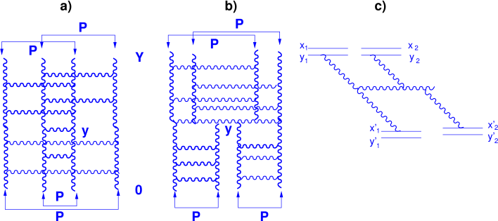
Figure 4: The diagrams for 2P to 2P process. Fig. 4-a shows the diagram which is of the order $\bar{\alpha}_{S}/N^{2}_{c}$ while Fig. 4-a leads to a contribution $\propto\bar{\alpha}^{3}_{S}$. Fig. 4-c shows the first diagram for the 2 dipole to 2 dipole amplitude which square gives the probability for 2P to 2P process.

The situation with $V_{2\to 1}$ is actually more dramatic since even in this paper we have discussed four different expression for this vertex:(i)   Eq. (3.75);   (ii)   Eq. (2.39) leads to the vertex of the following form (see Refs. [22, 23, 20] where this form of the vertex has been discussed in details)

$$\Gamma_{2\to 1}(x_{1},y_{1};x_{2},y_{2}|x,y)\,\,=\nabla^{2}_{x}\,\nabla^{2}_{y}\,\int\,d^{2}zK(x,y;z)\,\,G_{0}(x_{1},y_{1}|x,z)\,G_{0}(x_{1},y_{1}|z,y);$$ (4.99)

(iii)  Eq. (3.56) leads to

$$\Gamma_{2\to 1}(x,z;z,y|x,y)\,\,=\,\,K\left(x,y|z\right)$$ (4.100)

and the expression for vertex $V_{2\to 1}$ one can obtain substituting Eq. (4.100) into Eq. (3.75);   (iv)   Eq. (3.56) suggests the simple vertex

$$V_{2\to 1}(b,k;b,k|b,k)\,\,=\,\,\left(\frac{4\,\pi^{2}\,\bar{\alpha}_{S}}{N_{c}}\right)^{2}\,\frac{\bar{\alpha}_{S}}{2\,\pi}.$$ (4.101)

These expressions are equivalent in the framework of the BFKL Pomeron calculus but lead to quite different physics. For example, Eq. (4.99) does not generate $2\to 2$ dipole term in the functional integral [27] and, therefore, the noise term has a form of Eq. (3.61), while all other expression correspond to the noise term of Eq. (3.62) which belongs to a different universality class.

As we have mentioned that in the kinematic region where $L(Y)\approx 1$ (see Eq. (2.10)) the $2P\to 2P$ transitionj gives only neglitransitionibution. However, it changes crucially the behaviour of the scattering amplitude at ultra high energy.

Our strategy of the discussion looks as follows. First, we are going to discuss the two Pomeron to one Pomeron transition directly in terms of the dipole approach calculating Feyman diagrams. The key question that we want to answer is what process of the dipole recombination is described by the diagram that contribute to the $2P\to P$ vertex. Second, we wish to find what term in $\chi[u]$ (see Eq. (3.71)) is responsible for this contribution. Third, we find the solution for the toy model that includes this term. Finally, we develop the generating functional approach for the approach that correspond to the action given by Eq. (3.58) which we think will be a practical way in searching the solution.

4.2 Scattering of two dipoles in QCD

We start to approach the problem of taking into account the two Pomerons to two or more Pomerons transition with the clear understanding of $2P\to P$ merging in the dipole approach. In this section we will obtain the same Eq. (2.40) for $\Gamma_{2\to 1}$ but directly from the dipole picture of interaction without using the trick suggested in Ref. [22]. Namely, we will calculate the contribution of the simple diagrams like that of Fig. 18-a but directly from the dipole picture of interaction [17] shown in Fig. 18-b.

Starting to calculate the diagram of Fig. 18 we would like to draw your attention to the fact that these diagrams actually describe three different processes. In the Born approximation all of them look quite similar but if you imagine, that gluon with momentum $k$ and $l$ can produce more gluons (see dotted lines in Fig. 18, Fig. 19 and Fig. 20) , we can see a great difference between three diagrams. Indeed, the diagram of Fig. 18 represents the process where two bunches of additional gluons could be produced from gluons with momenta $\vec{k}_{\perp}$ and $\vec{l}_{\perp}$. This diagrams give a positive contribution and has clear probabilistic interpretation. Fig. 20 shows the process where none of additional gluons can be produced. The gluons, that were produced in the process of the diagrams of Fig. 18, contribute to the structure of the BFKL Pomerons. The diagram of Fig. 19 corresponds to a process where only one of the bunches of gluons is produced while the second one is absorbed by the BFKL Pomeron. This diagram belongs to an interference type of the diagram which can have a negative sign.

It is clear that these extra diagrams correspond to different AGK cuts of the BFKL Pomeron diagrams. Fortunately, they differs by the factor and sign in front of the same expression [41], namely,

$${Fig.~{}\ref{v212pic}}\,\,:\,\,{Fig.~{}\ref{v211pic}}\,\,:\,\,{Fig.~{}\ref{v21pic}}\,\,=\,\,1\,\,:\,\,-4\,\,:\,\,2$$ (4.102)

Before approaching our problem we want to show how one can calculate well known Lipatov vertex using light cone perturbation theory. The calculations are performed in the infinite momentum frame, large $N_{c}$, eikonal and Regge limits ([42, 43].

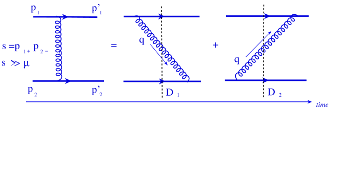
Figure 5: The diagram for the gluon exchange in the infinite momentum frame. The first diagram survives while the second one gives a small, negligible contribution at high energies.

We re-calculate the simplest diagram of one gluon exchange in the infinite momentum frame technique to illustrate the simple space-time structure of the high energy scattering that first have been formulated by Feynman and Gribov [42, 44].

It is well know that the one gluon exchange in Feynman diagram approach is equal to

$$A_{G}\,\,=\,\,\frac{\Gamma_{\mu}\,\Gamma_{\mu}}{q^{2}_{\perp}}$$ (4.103)

In the infinite momentum frame we need to sum the contributions of two diagrams shown in Fig. 5 which are equal to

$$D_{1} = \frac{\Gamma_{\mu}\,\Gamma_{\mu}}{2\,E_{q}}\,\frac{1}{E_{p_{1}}\,+\,E_{p_{2}}\,-\,E_{p_{2}}\,-\,E_{p^{\prime}_{1}}\,-\,E_{q}}\,\,=\,\,\frac{\Gamma_{\mu}\,\Gamma_{\mu}}{2\,E_{q}}\,\frac{1}{-\frac{p^{\prime 2}_{1,\perp}}{2\,p^{\prime}_{1,L}}\,\,-\,\,\frac{q^{2}_{\perp}}{q_{L}}}\,\,|_{s\ll\mu}\rightarrow\,\,\,\frac{\Gamma_{\mu}\,\Gamma_{\mu}}{q^{2}_{\perp}}\,;\,$$ (4.104)

$$D_{1} = \frac{\Gamma_{\mu}\,\Gamma_{\mu}}{2\,E_{q}}\,\frac{1}{E_{p_{1}}\,+\,E_{p_{2}}\,-\,E_{p^{\prime}_{2}}\,-\,E_{p_{1}}\,-\,E_{q}}\,\,\approx\,\,\frac{\Gamma_{\mu}\,\Gamma_{\mu}}{2\,E_{q}}\,\frac{1}{2E_{q}}\,\,\propto\,\,O(1/s)\,\ll 1;$$ (4.105)

The difference between these two diagrams is the following. The first one describes the process with natural ordering in time. Indeed, the typical time for the relativistic particles is $E/p^{2}_{\perp}$ where $E$ is the energy of the particle and $p_{\perp}$ is its transverse momentum. Therefore, the first diagram describes the process of the emission of long living gluon with the lifetime  $\tau_{q}\,\propto\,E_{q}/q^{2}_{\perp}$ by the parent particle with its lifetime $\tau_{p_{1}}\,\propto\,E_{p_{1}}/p^{2}_{1,\perp}\,\gg\,\tau_{q}$. In the second diagram, the particle with short lifetime $\tau_{p_{2}}\,\propto\,E_{p_{2}}/p^{2}_{2,\perp}\,\,\ll\,\,\tau_{q}$ emits the gluon with larger typical time. For emission of large number of gluons we have a space-time picture shown in Fig. 6. The square of these ladder-time diagram we will call the BFKL Pomeron. The general feature of this diagrams that the cross section can be written as the product of two factors: the square of the multi-gluon wave function ($\Psi$) and the cross section of the interaction of the slowest,‘wee’ gluon with the target

$$\sigma\,\,=\,\,|\Psi|^{2}\bigotimes\sigma(Gluon-target)$$ (4.106)

where $\bigotimes$ stands for integration over all kinematic variables of the wee gluon and $|\Psi|^{2}$ is the wavefunction integrated over all kinematic variables of the gluons that are faster than the wee one.

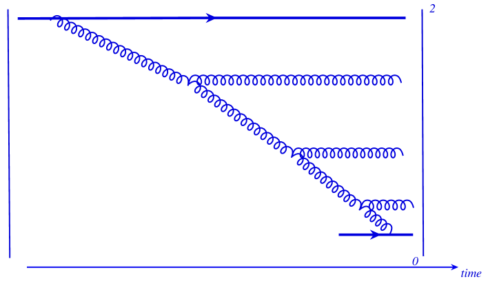
Figure 6: The space-time structure of the BFKL Pomeron in QCD.

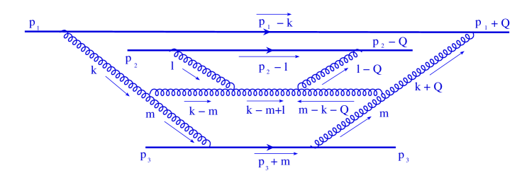
Figure 7: The total cross section of two quarks on one scattering

Figure 8: A diagram contributing to the effective vertex.

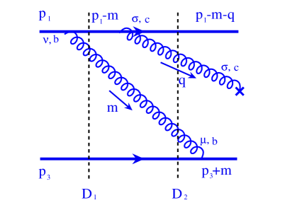
Figure 9: A diagram having relative $m_{-}$ suppression comparing to Fig. 9.

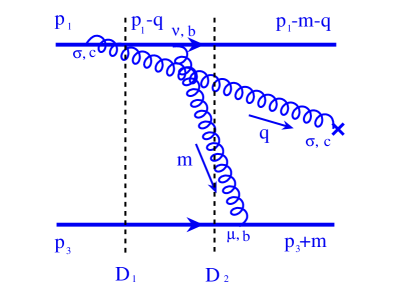
Figure 10: A diagram contributing to the effective vertex.

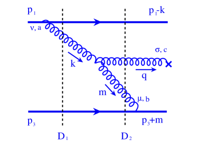
Figure 11: A diagram contributing to the effective vertex.

Before starting our calculations we want to show that this kind of diagrams indeed give the leading logarithm contribution. We consider the total cross section shown in Fig. 7.

We want to perform the integration over plus and minus components of all internal momenta leaving the transverse integration. It is convenient to do the integration in terms of Sudakov parameters on the complex plain. We assume the Regge limit, $p^{\mu}_{1}p_{3\mu}\simeq p^{\mu}_{2}p_{3\mu}=s/2$ and forward scattering, i.e. $Q_{\perp}=0$. Thus the internal momenta can be written as

$$k^{\mu} = \alpha_{k}p^{\mu}_{1}+\beta_{k}p^{\mu}_{3}+k_{\perp}^{\mu}$$

$$l^{\mu} = \alpha_{l}p^{\mu}_{1}+\beta_{l}p^{\mu}_{3}+l_{\perp}^{\mu}$$

$$m^{\mu} = \alpha_{m}p^{\mu}_{1}+\beta_{m}p^{\mu}_{3}+m_{\perp}^{\mu}$$ (4.107)

The total cross section have denominators that come from gluon propagators

$$k^{2}=\alpha_{k}\beta_{k}s-k_{\perp}^{2}$$ (4.108)

$$m^{2}=\alpha_{m}\beta_{m}s-m_{\perp}^{2}$$ (4.109)

$$l^{2}=\alpha_{l}\beta_{l}s-l_{\perp}^{2}$$ (4.110)

$$(k-m)^{2}=(\alpha_{k}-\alpha_{m})(\beta_{k}-\beta_{m})s-(k-m)_{\perp}^{2}$$ (4.111)

$$(l-Q)^{2}=(\alpha_{l}-\alpha_{Q})(\beta_{l}-\beta_{Q})s-l_{\perp}^{2}$$ (4.112)

$$(k+Q)^{2}=(\alpha_{k}+\alpha_{Q})(\beta_{k}+\beta_{Q})s-k_{\perp}^{2}$$ (4.113)

$$(k-m+Q)^{2}=(\alpha_{k}-\alpha_{m}+\alpha_{Q})(\beta_{k}-\beta_{m}+\beta_{Q})s-(k-m)_{\perp}^{2}$$ (4.114)

and the $\delta$-functions (from the cuts) of

$$(p_{2}-l)^{2} = -\beta_{l}s-l^{2}_{\perp}$$ (4.115)

$$(p_{1}-k)^{2} = -\beta_{k}s-k^{2}_{\perp}$$ (4.116)

$$(p_{3}+m)^{2} = \alpha_{m}s-m^{2}_{\perp}$$ (4.117)

In forward scattering the transverse part of the transferred momenta is zero ($Q_{\perp}=0$ ), from the on-shellness of the outgoing quarks it can be seen that $\alpha_{Q}$ and $\beta_{Q}$ can be neglected in further calculations. According to the Cutkosky rule the amplitude should be squared and integrated over all internal momenta. If the integration is performed in terms of Sudakov parameters it reads

$$d^{4}k\;d^{4}l\;d^{4}m=(\frac{s}{2})^{3}d\alpha_{k}\;d\beta_{k}\;d\alpha_{l}\;d\beta_{l}\;d\alpha_{m}\;d\beta_{m}\;d^{2}k_{\perp}\;d^{2}l_{\perp}\;d^{2}m_{\perp}$$ (4.118)

The integration over transverse momenta do not bring the leading logarithm of energy and thus may be omitted in our discussion of the origin of the $\ln s$ contribution.

First we do the integration with respect to $\beta_{k}$ which gives $\beta_{k}=-k^{2}_{\perp}/s$ and factor $-1/s$ from $\delta^{4}((p_{1}-k)^{2})$ (see Eq. 4.115 ). Next the integration over $\beta_{l}$ is performed, this gives at $\beta_{l}=-l^{2}_{\perp}/s$ and factor $-1/s$ from $\delta^{4}((p_{2}-l)^{2})$. The $\delta$-function of $(p_{3}+m)^{2}$ gives $\alpha_{m}=+m^{2}_{\perp}/s$ and factor $1/s$. For $t$-channel gluons the propagators can be written as follows

$$k^{2} = \alpha_{k}\beta_{k}s-k_{\perp}^{2}=\alpha_{k}(\frac{-k^{2}_{\perp}}{s})s-k_{\perp}^{2}\simeq-k_{\perp}^{2}$$ (4.119)

$$m^{2} = \alpha_{m}\beta_{m}s-m_{\perp}^{2}=\frac{m^{2}_{\perp}}{s}\beta_{m}s-m_{\perp}^{2}\simeq-m_{\perp}^{2}$$ (4.120)

$$l^{2} = \alpha_{l}\beta_{l}s-l_{\perp}^{2}=\alpha_{l}(\frac{-l^{2}_{\perp}}{s})s-l_{\perp}^{2}\simeq-l_{\perp}^{2}$$ (4.121)

Similarly one finds that $(k+Q)^{2}\simeq-k_{\perp}^{2}$, $(l-Q)^{2}\simeq-l_{\perp}^{2}$ .

After this we proceed to calculation of other denominators are given by

$$(k-m)^{2} = (\alpha_{k}-\alpha_{m})(\beta_{k}-\beta_{m})s-(k-m)^{2}_{\perp}=$$

$$(\alpha_{k}-\frac{m^{2}_{\perp}}{s})(-\frac{k^{2}_{\perp}}{s}-\beta_{m})s-(k-m)^{2}_{\perp}=\alpha_{k}\beta_{m}-(k-m)^{2}_{\perp}$$

and the integration with respect to $\alpha_{k}$ is done on the complex plain adding to denominator of Eq. 4.2 some small $i\epsilon$. The contour integration gives a residue at $\alpha_{k}=[(k-m)^{2}_{\perp}-i\epsilon]/\beta_{m}s$ and the factor $1/[\beta_{m}s]^{2}$ before the amplitude ($\beta^{2}_{m}$ squared is because of the propagator of gluon $m-k-Q$). Next, $(k-m+l)^{2}$ gives $\alpha_{l}=[(k-m+l)^{2}_{\perp}-i\epsilon]/\beta_{m}$ and another factor if $1/\beta_{m}s$.

We are left with some function of only transverse variables times $d\beta_{m}/\beta^{3}_{m}$. If we notice that the two triple gluon vertices in the center of Fig. 7 result into $\beta^{2}_{m}$ in the numerator (see Eq. 4.140 ) canceling two powers of $\beta_{m}$, than we end up with $d\beta_{m}/\beta_{m}$ which brings the logarithm of the energy.

We start with three types of diagrams of quark-quark scattering contributing to the effective vertex (see Fig. 9- 11). This result will be useful for our further considerations. The amplitude depicted of Fig. 9 reads as

$$g^{3}\frac{\bar{u}(p_{1})}{\sqrt{p_{1+}}}\gamma^{\nu}t^{b}\frac{u(p_{1}-m)}{\sqrt{p_{1+}-m_{+}}}\frac{-g_{\mu\nu}}{m_{+}}\frac{1}{D_{1}}\frac{\bar{u}(p_{1}-m)}{\sqrt{p_{1+}-m_{+}}}\gamma^{\sigma}t^{c}\frac{u(p_{1}-m-q)}{\sqrt{p_{1+}-m_{+}-q_{+}}}\frac{\bar{u}(p_{3})}{\sqrt{p_{3-}}}\gamma^{\mu}t^{b}\frac{1}{D_{2}}\frac{u(p_{3}+m)}{\sqrt{p_{3-}+m_{-}}}\epsilon^{q}_{\sigma}$$ (4.123)

where $D_{1}$ and $D_{2}$ are given by

$$D_{1}\,\, = \,\,p_{1-}+p_{3-}-\frac{(p_{1}-m)^{2}_{\perp}}{p_{1+}-m_{+}}-\frac{m^{2}_{\perp}}{m_{+}}-p_{3-}\simeq-\frac{m^{2}_{\perp}}{m_{+}}$$

$$D_{2} = p_{1-}+p_{3-}-\frac{(p_{1}-m)^{2}_{\perp}}{p_{1+}-m_{+}}-\frac{(p_{3}+m)^{2}_{\perp}}{p_{3+}+m_{+}}=$$

$$\frac{(p_{1}-m-q)^{2}_{\perp}}{p_{1+}-m_{+}-q_{+}}+\frac{(p_{3}-m)^{2}_{\perp}}{p_{3+}-m_{+}}-\frac{(p_{1}-m)^{2}_{\perp}}{p_{1+}-m_{+}}-\frac{(p_{3}+m)^{2}_{\perp}}{p_{3+}+m_{+}}\simeq+\frac{q^{2}_{\perp}}{q_{+}}$$

In estimates of $D_{2}$ we used the fact that initial light cone energy equals final light cone energy at high energies. Summing Eq.(4.123) over quark polarizations (see Ref. [43]) we have contribution only from plus and minus components of $\gamma^{\nu}$ and $\gamma^{\mu}$ respectively. Namely,

$$\frac{\bar{u}(p)}{\sqrt{p_{+}}}\gamma^{\mu}\frac{u(p-m)}{\sqrt{p_{+}-m_{+}}}=n^{\mu}$$ (4.125)

where $n^{\mu}$ is defined such that $n^{\mu}k_{\mu}=k_{-}$ for an arbitrary 4-vector $k^{\mu}$. Now we can rewrite Eq.4.123 as

$$t^{b}t^{c}\otimes t^{b}g^{3}n_{+}n_{-}\frac{q_{-}}{q^{2}_{\perp}}\frac{-m_{+}}{m^{2}_{\perp}}\frac{-1}{m_{+}}\epsilon_{-}=t^{b}t^{c}\otimes t^{b}g^{3}2\frac{q_{+}}{q_{\perp}^{2}}\frac{1}{m_{\perp}^{2}}\epsilon_{-}=t^{b}t^{c}\otimes t^{b}4\frac{1}{m_{\perp}^{2}}\frac{q_{\perp}\epsilon_{\perp}}{q_{\perp}^{2}}$$ (4.126)

Here we used the transverse condition

$$q^{\mu}\epsilon^{q}_{\mu}=\frac{1}{2}q_{+}\epsilon^{q}_{-}-q_{\perp}\epsilon^{q}_{\perp}=0\;\;\;\longrightarrow\;\;\;\epsilon_{-}=2\frac{q_{\perp}\epsilon^{q}_{\perp}}{q_{+}}$$ (4.127)

One should consider another diagram depicted in Fig. 9, but it can be readily seen that both of its denominators are of the order of $D_{1}\,\approx\,\,D_{2}\,\,\approx\,m_{-}=m^{2}_{\perp}/m_{+}$. Thus it is has an additional $m_{-}$ suppression comparing to the amplitude of Fig. 9 which will not give the logarithmic contribution $\propto Y=\ln s$. Next we consider a diagram shown in Fig. 11 given by

$$g^{3}\frac{\bar{u}(p_{1})}{\sqrt{p_{1+}}}\gamma^{\sigma}t^{c}\frac{u(p_{1}-q)}{\sqrt{p_{1+}-q_{+}}}\frac{1}{D_{1}}\frac{\bar{u}(p_{1}-q)}{\sqrt{p_{1+}-q_{+}}}\gamma^{\nu}t^{b}\frac{u(p_{1}-m-q)}{\sqrt{p_{1+}-m_{+}-q_{+}}}\frac{\bar{u}(p_{2})}{\sqrt{p_{3-}}}\gamma^{\mu}t^{b}\frac{u(p_{2}+m)}{\sqrt{p_{3-}+m_{-}}}\frac{1}{D_{2}}\epsilon^{q}_{\sigma}$$ (4.128)

where $D_{1}$ and $D_{2}$ are given by

$$D_{1}\,\, = \,\,p_{1-}+p_{2-}-\frac{(p_{1}-q)^{2}_{\perp}}{p_{1+}-q_{+}}-\frac{q^{2}_{\perp}}{q_{+}}-p_{2-}\simeq-\frac{q^{2}_{\perp}}{q_{+}}$$

$$D_{2} = p_{1-}+p_{2-}-\frac{(p_{1}-m-q)^{2}_{\perp}}{p_{1+}-m_{+}-q_{+}}-p_{2-}\simeq-\frac{m^{2}_{\perp}}{m_{+}}$$ (4.129)

Summing over quark polarizations we get the resulting expression for the amplitude shown in Fig. 11

$$t^{c}t^{b}\otimes t^{b}g^{3}n_{+}n_{-}\frac{-q_{+}}{q_{\perp}^{2}}\frac{-m_{+}}{m_{\perp}^{2}}\frac{-1}{m_{+}}\epsilon_{-}=-t^{b}t^{c}\otimes t^{b}g^{3}2\frac{q_{+}}{q_{\perp}^{2}}\frac{1}{m_{\perp}^{2}}\epsilon_{-}=-t^{b}t^{c}\otimes t^{b}g^{3}4\frac{1}{m_{\perp}^{2}}\frac{q_{\perp}\epsilon_{\perp}}{q_{\perp}^{2}}$$ (4.130)

We see that the contribution of Fig. 11 is equal to that of Fig. 9 but opposite in sign. We also notice that they enter with different color matrices $t^{a}t^{b}\otimes t^{b}$ and $t^{b}t^{a}\otimes t^{b}$ respectively. Using the basic relation for Lie group generators $[t^{a},t^{b}]=if^{abc}t^{c}$ we can write the contribution from the two diagrams as

$$if^{abc}t^{c}\otimes t^{b}g^{3}4\frac{1}{m_{\perp}^{2}}\frac{q_{\perp}\epsilon_{\perp}}{q_{\perp}^{2}}$$ (4.131)

The last diagram to be considered is shown in Fig. 11 and given by

$$if^{abc}t^{c}\otimes t^{b}g^{3}\frac{\bar{u}(p_{1})}{\sqrt{p_{1+}}}\gamma^{\mu}\frac{\bar{u}(p_{1}-k)}{\sqrt{p_{1+}-k_{+}}}\frac{1}{D_{1}}\frac{-g_{\nu\nu^{\prime}}}{k_{+}}\Gamma^{\nu^{\prime}\mu^{\prime}\sigma}\frac{-g_{\mu\mu^{\prime}}}{m_{+}}\frac{1}{D_{2}}\frac{\bar{u}(p_{3})}{\sqrt{p_{3-}}}\gamma^{\mu}\frac{\bar{u}(p_{3}-m)}{\sqrt{p_{3-}-m_{+}}}\epsilon^{q}_{\sigma}$$ (4.132)

where $\Gamma^{\nu^{\prime}\mu^{\prime}\sigma}$ is a regular triple gluon QCD vertex.

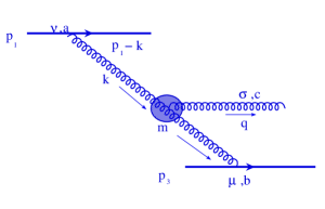
Figure 12: Schematic representation of the effective vertex.

The light cone energy denominators $D_{1}$ and $D_{2}$ are readily calculated

$$D_{1} = p_{1-}+p_{2-}-\frac{(p_{1}-k)^{2}_{\perp}}{p_{1+}-k_{+}}-\frac{k^{2}_{\perp}}{k_{+}}-p_{2-}\simeq-\frac{k^{2}_{\perp}}{k_{+}}$$

$$D_{2} = p_{1-}+p_{2-}-\frac{(p_{1}-k)^{2}_{\perp}}{p_{1+}-k_{+}}\frac{q^{2}_{\perp}}{q_{+}}-\frac{m^{2}_{\perp}}{m_{+}}-p_{2-}\simeq-\frac{m^{2}_{\perp}}{m_{+}}$$ (4.133)

The triple gluon vertex can be reduced as follows (see [1])

$$\Gamma^{\nu^{\prime}\mu^{\prime}\sigma} = g[g^{\nu^{\prime}\mu^{\prime}}(k+m)^{\sigma}+g^{\mu^{\prime}\sigma}(-m+q)^{\nu^{\prime}}+g^{\nu^{\prime}\sigma}(-q-k)^{\mu^{\prime}}]$$ (4.134)

$$= [g^{\nu^{\prime}\mu^{\prime}}2k^{\sigma}+g^{\mu^{\prime}\sigma}(-m+q)^{\nu^{\prime}}-g^{\nu^{\prime}\sigma}2k^{\mu^{\prime}}]\simeq g^{\nu^{\prime}\mu^{\prime}}2k^{\sigma}$$

With these simplifications Eq. 4.132 can be written as follows

$$if^{abc}t^{c}\otimes t^{b}g^{3}n_{+}n_{-}\frac{-k_{+}}{k_{\perp}^{2}}\frac{-m_{+}}{m_{\perp}^{2}}\frac{-1}{m_{+}}\frac{-1}{k_{+}}2k^{\sigma}\epsilon^{q}_{\sigma}=if^{abc}t^{c}\otimes t^{b}g^{3}4\frac{1}{m_{\perp}^{2}}\frac{k_{\perp}\epsilon_{\perp}}{k_{\perp}^{2}}$$ (4.135)

The resulting contribution from diagrams Figs. 9-11 is schematically shown in Fig.12 and reproduces the effective Lipatov vertex

$$if^{abc}t^{c}\otimes t^{b}g^{3}4\frac{1}{m_{\perp}^{2}}\left(\frac{k_{\perp}\epsilon_{\perp}}{k_{\perp}^{2}}-\frac{q_{\perp}\epsilon_{\perp}}{q_{\perp}^{2}}\right)$$ (4.136)

We continue with the light cone perturbation theory and consider a second quark emitting gluon $l$ that hits gluon $q$, as shown in Fig. 13. It is worth mentioning that the gluons $l$ and $q$ should be coupled to the quark $1$ and quark $2$ lines via the effective vertex found before. For simplicity, we consider only one type of the diagrams contributing in this case and generalize the result to all the possible couplings. There exists a lot of ways to perform the light cone energy cut when one adds second scattering quark. As it was shown before that cuts double the same lower gluon are suppressed in Regge limit. The amplitude shown in Fig. 13 is written as follows

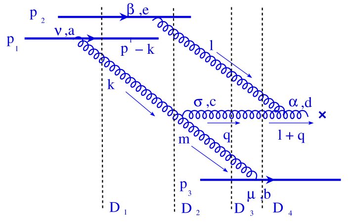
Figure 13: One of the diagrams contributing to 2P $\rightarrow$ P vertex calculated in light cone perturbation theory

$$\frac{\bar{u}(p_{1})}{\sqrt{p_{1+}}}\gamma^{\nu}\frac{u(p_{1}-k)}{\sqrt{p_{1+}-k_{+}}}\frac{-g_{\nu\nu^{\prime}}}{k_{+}}\frac{1}{D_{1}}\frac{\bar{u}(p_{2})}{\sqrt{p_{2+}}}\gamma^{\mu}\frac{u(p_{2}-l)}{\sqrt{p_{2+}-l_{+}}}\frac{-g_{\beta\beta^{\prime}}}{l_{+}}\frac{1}{D_{2}}$$

$$\Gamma^{\nu^{\prime}\mu^{\prime}\sigma}\frac{1}{D_{3}}\frac{\bar{u}(p_{3})}{\sqrt{p_{3+}}}\gamma^{\beta}\frac{-g_{\mu\mu^{\prime}}}{m_{+}}\frac{u(p_{3}-m)}{\sqrt{p_{3-}-m_{-}}}\frac{-g_{\sigma\sigma^{\prime}}}{q_{+}}\frac{1}{D_{4}}\Gamma^{\sigma^{\prime}\beta^{\prime}\alpha}\epsilon^{q+l}_{\alpha}$$ (4.137)

where the denominators $D_{1}$-$D_{4}$ are given by

$$D_{1} \,\,=\,\, p_{1-}+p_{2-}+p_{3-}-\frac{(p_{1}-k)^{2}_{\perp}}{p_{1+}-k_{+}}-\frac{k^{2}_{\perp}}{k_{+}}-p_{2-}-p_{3-}\simeq-\frac{k^{2}_{\perp}}{k_{+}}$$

$$D_{2} = p_{1-}+p_{2-}+p_{3-}-\frac{(p_{1}-k)^{2}_{\perp}}{p_{1+}-k_{+}}-\frac{k^{2}_{\perp}}{k_{+}}-\frac{(p_{2}-l)^{2}_{\perp}}{p_{2+}-l_{+}}-\frac{l^{2}_{\perp}}{l_{+}}-p_{3-}\simeq-\frac{l^{2}_{\perp}}{l_{+}}$$ (4.138)

$$D_{3} = p_{1-}+p_{2-}+p_{3-}-\frac{(p_{1}-k)^{2}_{\perp}}{p_{1+}-k_{+}}-\frac{q^{2}_{\perp}}{q_{+}}-\frac{m^{2}_{\perp}}{m_{+}}-\frac{(p_{2}-l)^{2}_{\perp}}{p_{2+}-l_{+}}-\frac{l^{2}_{\perp}}{l_{+}}-p_{3-}\simeq-\frac{m^{2}_{\perp}}{m_{+}}$$

$$D_{4} = p_{1-}+p_{2-}+p_{3-}-\frac{(p_{1}-k)^{2}_{\perp}}{p_{1+}-k_{+}}-q_{-}-\frac{(p_{2}-l)^{2}_{\perp}}{p_{2+}-l_{+}}-\frac{l^{2}_{\perp}}{l_{+}}-\frac{(p_{3}-m)^{2}_{\perp}}{p_{3+}-m_{+}}\simeq-q_{-}$$

In Eq. 4.2 we omitted coupling constants and color factors that will be easily restored at the end of the calculations. The amplitude Eq. 4.2 can be further simplified as follows

$$n^{\nu}\frac{-g_{\nu\nu^{\prime}}}{k_{+}}\frac{-k_{+}}{k^{2}_{\perp}}n^{\mu}\frac{-g_{\beta\beta^{\prime}}}{l_{+}}\frac{-l_{+}}{l^{2}_{\perp}}\Gamma^{\nu^{\prime}\sigma\alpha^{\prime}}\frac{-m_{+}}{m^{2}_{\perp}}\frac{-g_{\mu\mu^{\prime}}}{m_{+}}\tilde{n}^{\beta}\frac{-g^{\sigma\sigma^{\prime}}}{q_{+}q_{-}}\Gamma^{\sigma^{\prime}\beta^{\prime}\alpha}\epsilon^{q+l}_{\alpha}$$ (4.139)

where vector $\tilde{n}^{\beta}$ is defined as $\tilde{n}^{\beta}k_{\beta}=k_{-}$ for any arbitrary vector $k^{\beta}$. The triple gluon QCD vertex $\Gamma^{\nu^{\prime}\sigma\alpha^{\prime}}$ is given in Eq. 4.134. The vertex $\Gamma^{\sigma^{\prime}\beta^{\prime}\alpha}$ in our case can be simplified as follows

$$\Gamma^{\sigma^{\prime}\beta^{\prime}\alpha}=g^{\alpha\beta^{\prime}}(l-q)^{\sigma^{\prime}}+g^{\alpha\sigma^{\prime}}(2q+l)^{\beta^{\prime}}+g^{\beta^{\prime}\sigma^{\prime}}(-q-2l)^{\alpha}\simeq g^{\alpha\sigma^{\prime}}(2q+l)^{\beta^{\prime}}$$ (4.140)

Using this we rewrite Eq. 4.139 as

$$+n^{2}2\frac{1}{k^{2}_{\perp}}\frac{1}{l^{2}_{\perp}}\frac{1}{m^{2}_{\perp}}\frac{(2q+l)_{-}}{q_{+}q_{-}}k^{\alpha}\epsilon^{q+l}_{\alpha}\simeq-2\cdot 2\frac{1}{k^{2}_{\perp}}\frac{1}{l^{2}_{\perp}}\frac{1}{m^{2}_{\perp}}\frac{2}{q_{+}}k_{\perp}\cdot\epsilon^{q+l}_{\perp}$$ (4.141)

We note a plus component of $q$ in the denominator, this factor is not related to integration in transverse coordinates and leads to a logarithm of energy as was shown before for total cross section, thus it can be omitted at this stage and safely restored at the end of the calculations. Performing similar transformations for an amplitude of two gluons being emitted from quark (antiquark) lines (see Fig. 9- 11) we get

$$+2\cdot 2\frac{1}{q^{2}_{\perp}}\frac{1}{l^{2}_{\perp}}\frac{1}{m^{2}_{\perp}}2q_{\perp}\cdot\epsilon^{q+l}_{\perp}$$ (4.142)

with the same color factor as of Eq. 4.141.Thus, Fig. 13 gives

$$8\frac{1}{l^{2}_{\perp}}\frac{1}{m^{2}_{\perp}}\left(\frac{k_{\perp}^{\alpha}}{k_{\perp}^{2}}-\frac{q_{\perp}^{\alpha}}{q_{\perp}^{2}}\right)$$ (4.143)

One should add another one, where momenta $q$ and $l$ are interchanged, to this expression, then it gives an effective vertex for the scattering of two with one quarks (with color factor, powers of $g$ and plus-minus components restored). Now we want to find the cross section that corresponds to two dipoles being scattered with a target. We use a mixed representation where we Fourier transform all transverse momenta to coordinates of dipoles (quarks). We assign transverse coordinates $x_{i}$ ($y_{i}$) to each quark (antiquark) line, and coordinate $z$ for the emitted gluon. The Fourier transform is performed separately for $d^{2}k_{\perp}$ and $d^{2}q_{\perp}$ integrations . We start with Eq. 4.141

$$\int\frac{d^{2}k_{\perp}}{(2\pi)^{2}}\frac{d^{2}l_{\perp}}{(2\pi)^{2}}\frac{d^{2}m_{\perp}}{(2\pi)^{2}} e^{i(k-m+l)_{\perp}z}\left(e^{im_{\perp}x_{3}}-e^{im_{\perp}y_{3}}\right)\left(e^{-il_{\perp}x_{2}}-e^{-il_{\perp}y_{2}}\right)\times$$ (4.144)

$$\times \left(e^{-ik_{\perp}x_{1}}-e^{-ik_{\perp}y_{1}}\right)8\frac{1}{l^{2}_{\perp}}\frac{1}{m^{2}_{\perp}}\frac{k_{\perp}^{\alpha}}{k^{2}_{\perp}}$$

To simplify Eq. 4.144 we introduce the gluon propagator in the coordinate space

$$D_{G}(x,x^{\prime})=\int\frac{d^{2}k_{\perp}}{(2\pi)^{2}}\frac{1}{k^{2}_{\perp}}e^{ik_{\perp}(x-x^{\prime})}=-\frac{\ln\left(|x-x^{\prime}|\mu\right)}{2\pi}$$ (4.145)

where $\mu$ is an arbitrary small mass that we need to send to $0$ at the end of our calculations, and the integral

$$\int\frac{d^{2}k_{\perp}}{(2\pi)^{2}}\frac{k_{\perp}^{\alpha}}{k^{2}_{\perp}}e^{ik_{\perp}(x-x^{\prime})}=\frac{i}{2\pi}\frac{(x-x^{\prime})^{\alpha}}{(x-x^{\prime})^{2}}$$ (4.146)

which will be interpreted later. In terms of Eq. 4.145 and Eq. 4.146 we can rewrite Eq. 4.144 as follows

$$\frac{i}{2\pi}\left[\frac{(z-x_{1})^{\alpha}}{(z-x_{1})^{2}}-\frac{(z-y_{1})^{\alpha}}{(z-y_{1})^{2}}\right]\left(D_{G}(z,x_{3})-D_{G}(z,y_{3})\right)\left(D_{G}(z,x_{2})-D_{G}(z,y_{2})\right)$$ (4.147)

In a similar way we rewrite Eq. 4.142 in the form of

$$\int\frac{d^{2}q_{\perp}}{(2\pi)^{2}}\frac{d^{2}l_{\perp}}{(2\pi)^{2}}\frac{d^{2}m_{\perp}}{(2\pi)^{2}}e^{i(q+l)_{\perp}z}\left(e^{im_{\perp}x_{3}}-e^{im_{\perp}y_{3}}\right)\left(e^{-il_{\perp}x_{2}}-e^{-il_{\perp}y_{2}}\right)\times$$

$$\left(e^{-iq_{\perp}x_{1}}-e^{-iq_{\perp}y_{1}}\right)\left(e^{-im_{\perp}x_{1}}-e^{-im_{\perp}y_{1}}\right)8\frac{1}{l^{2}_{\perp}}\frac{1}{m^{2}_{\perp}}\frac{-q_{\perp}^{\alpha}}{q^{2}_{\perp}}=-\frac{i}{2\pi}\left[\frac{(z-x_{1})^{\alpha}}{(z-x_{1})^{2}}-\frac{(z-y_{1})^{\alpha}}{(z-y_{1})^{2}}\right]\times$$

$$\left(D_{G}(x_{3},x_{1})-D_{G}(y_{3},x_{1})-D_{G}(x_{3},y_{1})+D_{G}(y_{3},y_{1})\right)\left(D_{G}(z,x_{2})-D_{G}(z,y_{2})\right)$$ (4.148)

Eqs. 4.147-4.2 should be multiplied by the wavefunctions of the original dipoles $\psi^{(0)}(x_{i},y_{i})$, their factors have transparent physical meaning, namely

$$\left[\frac{(z-x_{1})^{\alpha}}{(z-x_{1})^{2}}-\frac{(z-y_{1})^{\alpha}}{(z-y_{1})^{2}}\right]\hskip 28.45274pt\mbox{describes the emission of gluon $z$ by dipole $(x_{1},y_{1})$ }$$

(4.149)

$$\left(D_{G}(z,x_{3})-D_{G}(z,y_{3})\right)\hskip 28.45274pt\mbox{describes the interaction of gluon $z$ with target dipole $(x_{3},y_{3})$ }$$

It should be noted that Eq. 4.147 should be multiplied by $2$ before adding to Eq. 4.2. This could be explained as follows, let us go back from large $N_{c}$ limit to $N_{c}=3$ and add a color singlet corresponding to large $N_{c}$ limit. We want to consider a combinatorial factor for all possible emissions of two gluons from dipole $(x_{1},y_{1})$ (see Fig. 15- Fig. 17) fixing the colour in the final states. It is clearly seen from the picture that the upper figure that corresponds to Eq. 4.141, has as much as twice options for two gluons to be emitted.

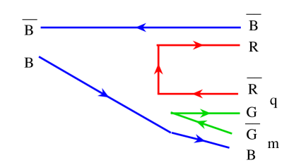
Figure 14: Colour structure of the reaction $q(blue)+\bar{q}(antiblue)\,\rightarrow\,q\bar{q}+G(q+m)\rightarrow q\bar{q}+G(q)+G(m)$. $B,G,R(\bar{B},\bar{G},\bar{R})$ stand for blue, green and red quarks (antiquarks), respectively.

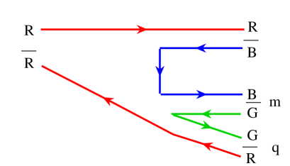
Figure 15: Colour structure of the reaction $q(red)+\bar{q}(antired)\,\rightarrow\,q\bar{q}+G(q+m)\rightarrow q\bar{q}+G(q)+G(m)$.$B,G,R(\bar{B},\bar{G},\bar{R})$ stand for blue, green and red quarks (antiquarks), respectively.labelCol2

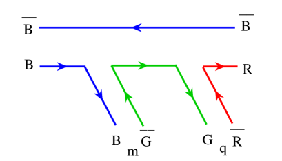
Figure 16: Colour structure of the reaction $q(blue)+\bar{q}(antiblue)\,\rightarrow\,q\bar{q}+G(q)+G(m)$. $B,G,R(\bar{B},\bar{G}B,G,R(\bar{B},\bar{G},\bar{R})$ stand for blue, green and red quarks (antiquarks), respectively.

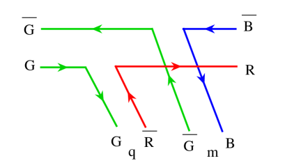
Figure 17: Colour structure of the reaction $q(green)+\bar{q}(antigreen)\,\rightarrow\,q\bar{q}+G(q)+G(m)$. $B,G,R(\bar{B},\bar{G},\bar{R})$ stand for blue, green and red quarks (antiquarks), respectively.

Using this fact we may add Eq. 4.147 to Eq. 4.2

$$-\frac{i}{2\pi}\left[\frac{(z-x_{1})^{\alpha}}{(z-x_{1})^{2}}-\frac{(z-y_{1})^{\alpha}}{(z-y_{1})^{2}}\right]\left(D_{G}(z,x_{1};x_{3},y_{3})+D_{G}(z,y_{1};x_{3},y_{3})\right)\left(D_{G}(z,x_{2})-D_{G}(z,y_{2})\right)$$ (4.150)

where $D_{G}(z,x_{1};x_{3},y_{3})$ stands for interaction of dipole $(z,x_{1})$ with the target. One should also add a term similar to Eq. 4.150 with dipole $1$ interchanged with dipole $2$ ($x_{1},y_{1}\leftrightarrow x_{2},y_{2}$). Now we are in position to square the summed diagrams. It can be easily shown that all types of interference terms vanish after the integration over $z$. Thus we are left with each term squared and the final expression reads as

$$|\psi^{(0)}(x_{1},y_{1})|^{2}|\psi^{(0)}(x_{2},y_{2})|^{2}|\psi^{(0)}(x_{3},y_{3})|^{2}\frac{\alpha_{s}N_{c}}{2\pi^{2}}\times$$ (4.151)

$$\int_{0}^{Y}dY^{\prime}\int d^{2}z\{2\gamma^{BA}(x_{2},y_{2}|z)K(x_{1},y_{1}|z)[\gamma^{BA}(x_{1},z|x_{3},y_{3})+\gamma^{BA}(y_{1},z|x_{3},y_{3})]+(1\leftrightarrow 2)\}$$

where $\gamma^{BA}(x,y|x^{\prime},y^{\prime})=(\frac{\alpha_{s}}{4\pi^{2}})^{2}G_{0}(x,y|x^{\prime},y^{\prime})$ with $G_{0}$ being the initial Green function given by Eq. 2.27, and $K(x,y|z)$ is given by Eq. 2.37. $\gamma^{BA}(x_{2},y_{2}|z)$ describes the interaction of a gluon with coordinate $z$ with dipole $(x_{2},y_{2})$ (see Fig. 21). It is equal to

$$\gamma^{BA}(x_{1},y_{1}|z)=\frac{1}{8}\left(\frac{\alpha_{s}}{2\pi}\right)^{2}\ln^{2}\left[\frac{(x_{1}-z)^{2}}{(y_{1}-z)^{2}}\right]$$ (4.152)

Eq. (4.151) should be multiplied by the factor $\ln s$ which is originated from the integration over the energy of produced gluon with the coordinate $z$.

One can see from Eq. (4.150) that we obtain the kernel of the BFKL equation for the interaction of one dipole $(x_{1},y_{1})$ in Fig. 18-d with the target dipole $(x,y)$ (see Fig. 18-a). Indeed, neglecting factor $D_{G}(x_{2},z)-D_{G}(z,y_{2})$ in Eq. (4.150) we have the following answer taking derivative with respect to $Y=\ln s$ from $|A({Eq.~{}(\ref{fig5exp12})})|^{2}$

$$\frac{d|A({Eq.~{}(\ref{fig5exp12})})|^{2}}{dY} \,\,=\,\,$$

$$= \,\frac{\bar{\alpha}_{S}}{2\pi}\int\,\,d^{2}z\,|\Psi_{0}(x_{2},y_{2})|^{2}\,K\left(x_{1},y_{1}|z\right)\,\,\left(\,\gamma^{BA}(x_{1},z|x_{3},y_{3})\,\,+\,\,\gamma^{BA}(z,y_{1}|x_{3},y_{3})\,\right)$$

In Eq. (4.2) one can recognize the BFKL equation with the kernel $\frac{\bar{\alpha}_{S}}{2\pi}\,\,K\left(x_{1},y_{1}|z\right)$.

4.3 Contribution to the generating functional

Eq. (4.151) gives the expression for the transition $(x_{1},y_{1})\,+\,(x_{2},y_{2})\,\,\rightarrow\,\,(x_{1},y_{2})\,+\,(x_{1},z)\,+\,(z,y_{1})$ given by the diagrams of Fig. 18-c and Fig. 18-d. This diagram gives a positive contribution but the sum of all diagrams (see Fig. 18, Fig. 19 and Fig. 20) leads to a negative contribution due to the AGK cutting rules (see Eq. (4.102)). The advantages of this direct calculations are clear: first, we obtain the vertex for $2\to 1$ transition in more convenient form than it was calculated before (see Refs. [22, 23, 20]). From Eq. (4.151) we see that this vertex is equal to

$$\Gamma_{2\to 1}\left((x_{1},y_{1})+(x_{2},y_{2})\to(x,y)\right)\,\,\,=\,\,\frac{\alpha_{S}N_{c}}{2\pi^{2}}\,\,\tilde{K}\left(x_{1},y_{1};x_{2},y_{2}|z\right)\,\,\,=\,\,$$ (4.154)

$$\,\,\frac{\alpha_{S}N_{c}}{2\pi^{2}}\,\,\left\{2\,\gamma^{BA}\left(x_{1},y_{1}|z\right)\times K\left(x_{2},y_{2};z\right)\,\,+\,\,x_{1}\leftrightarrow x_{2},y_{1}\leftrightarrow y_{2}\right\}$$

It should be stressed that Eq. (4.154) leads to a vertex which is positive in the full phase space.

The second advantage is that we can understand what process in terms of dipole these diagrams describe. Indeed, at initial rapidity $Y$ we have two colour dipoles:$(x_{1},y_{1})$ and $(x_{2},y_{2})$. The diagram of Fig. 21-a describes the transition of these two intitial dipoles which goes in two initial

$$(x_{1},y_{1})\,+\,(x_{2},y_{2})\,\,\rightarrow\,\,(x_{1},y_{1})\,+\,(x_{2},z)\,+\,(z,y_{2})\,\,\rightarrow\,\,(x_{1},y_{2})\,+\,(x_{2},z)\,+\,(z,y_{1});$$ (4.155)

and the target dipole $(x,y)$ interacts with dipoles: $(x_{2},z)$ and $(z,y_{2})$ during the first stage of the process or with $(x_{2},z)$ and $(z,y_{2})$ in the last stage.

Therefore, in terms of the functional of Eq. (3.2) these diagrams can be written as

$$-\,\frac{1}{2}\,\Gamma_{2\to 1}\left({Eq.~{}(\ref{V21N})}\right)\,\left(\gamma(x_{1},z)\,\,+\,\,\gamma(z,y_{1})\,\,+\,\,\gamma(x_{2},z)\,\,+\,\,\gamma(z,y_{2})\right)\,\frac{\delta}{\delta\gamma(x_{1},y_{1})}\,\frac{\delta}{\delta\gamma(x_{2},y_{2})}$$ (4.156)

The form of Eq. (4.156) suggests that this term can be originated by the following term in the Hamiltonian $\chi[u]$ (see Eq. (3.69) and Eq. (3.71)) :

$$\frac{1}{2}\,\Gamma_{2\to 1}\left({Eq.~{}(\ref{V21N})}\right)\,\left[u(x_{1},z)\,u(z,y_{1})\,\,+\,\,u(x_{2},z)\,u(z,y_{2})\right]\,\,\frac{\delta}{\delta u(x_{1},y_{1})}\,\frac{\delta}{\delta u(x_{2},y_{2})}$$ (4.157)

The Feynman diagrams that correspond to this term are shown in Fig. 4-b and Fig. 4-c. However, Eq. (4.157) cannot be correct since it leads to a positive two dipoles to two dipole amplitude. Indeed, for two dipoles to two dipole amplitude we have the same three diagrams of Fig. 18, Fig. 19 and Fig. 20 types. The sum of these diagrams gives the negative sign (see Ref. [39] where this problem was studied in details ).

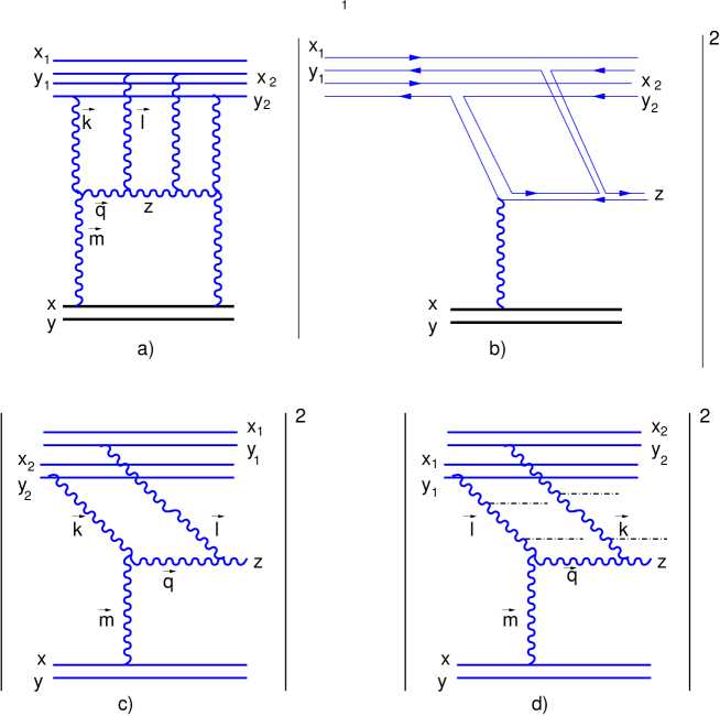
Figure 18: The diagram of the 2 Pomeron into one Pomeron transition and its dipole interpretation: diagonal contribution.

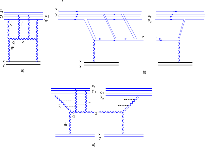
Figure 19: The diagram of the 2 Pomeron into one Pomeron transition and its dipole interpretation: non-diagonal contribution with elastic rescattering of the dipole $x_{1},y_{1}$).

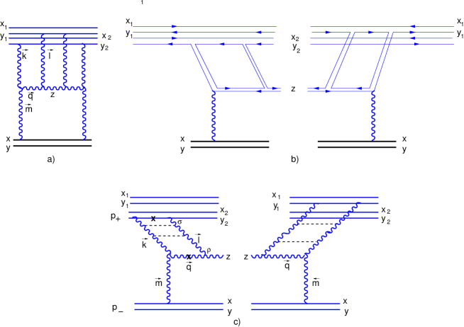
Figure 20: The diagram of the 2 Pomeron into one Pomeron transition and its dipole interpretation: non-diagonal contribution with the interference between the decays of two dipoles.

Repeating the same calculation which we made, summing Fig. 18,Fig. 19 and Fig. 20, one obtain for $2\to 2$ dipole amplitude the following answer

$$-\frac{1}{2}\,\Gamma_{2\to 1}\left({Eq.~{}(\ref{V21N})}\right)\,\left\{\gamma(x_{1},z)(\gamma(z,y_{1})\,\,+\,\,\gamma(x_{2},z)\,\,+\,\,\gamma(z,y_{2}))\,+\right.$$ (4.158)

$$\left.\,\gamma(x_{2},z)(\gamma(z,y_{1})\,+\,\gamma(z,y_{2}))\,+\,\gamma(z,y_{1})\gamma(z,y_{2})\right\}\,\frac{\delta}{\delta\gamma(x_{1},y_{1})}\,\frac{\delta}{\delta\gamma(x_{2},y_{2})}$$

Eq. (4.154) and Eq. (4.158) suggest that all dipoles that have been produced in both stages of the process (see Eq. (4.155)) interact with the target. It means that the contribution to $\chi[u]$ (see Eq. (3.69) and Eq. (3.71)) looks as follows

$$-\frac{1}{2}\,\Gamma_{2\to 1}\left({Eq.~{}(\ref{V21N})}\right)\,u(x_{2},z)\,u(z,y_{2})\,u(x_{1},y_{2})\,u(z,y_{1})\,\frac{\delta}{\delta u(x_{1},y_{1})}\,\frac{\delta}{\delta u(x_{2},y_{2})}$$ (4.159)

Eq. (4.159) describes the process of decay of two dipoles into four dipoles. As one can see from Eq. (3.66) - Eq. (3.68) each process for the dipole transition generates two terms in Markov’s chain which lead in Eq. (3.66) - Eq. (3.68) to the positive contribution which represents the increase in the number of dipoles due to the elementary process ( birth term)and a negative contribution which describes a decrease of the number of dipoles as a result of the elementary process (death term). The death term which corresponds to the birth term given by Eq. (4.159) has the form

$$-\frac{1}{2}\,\int\,\,d^{2}z\,\,\Gamma_{2\to 1}\left({Eq.~{}(\ref{V21N})}\right)\,u(x_{1},y_{1})\,\,u(x_{2},y_{2})\,\,\frac{\delta}{\delta u(x_{1},y_{1})}\,\frac{\delta}{\delta u(x_{2},y_{2})}$$ (4.160)

where

$$\int\,\,d^{2}z\,\,\Gamma_{2\to 1}\left({Eq.~{}(\ref{V21N})}\right)\,\,=\,\,$$ (4.161)

$$\frac{\alpha_{S}N_{c}}{2\pi^{2}}\,\,\left\{2\,\left(\gamma^{BA}\left(x_{1},y_{1}|x_{2}\right)\,,\,+\,\,\gamma^{BA}\left(x_{1},y_{1}|y_{2}\right)\right)\times\int\,d^{2}z\,\,K\left(x_{2},y_{2};z\right)\,\,+\,\,x_{1}\leftrightarrow x_{2},y_{1}\leftrightarrow y_{2}\right\}$$

It is easy to see that for the case when two dipoles are the same, Eq. (4.160) describes the diagram of Fig. 22

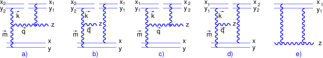
Figure 21: The diagrams for the amplitude of two dipole with one dipole interaction with emission of one extra gluon.

Figure 22: The diagrams for the amplitude which describes the death term in the equation for the generating functional in the case when dipoles $(x_{1},y_{1})$ and $(x_{2},y_{2})$ are equal.

Finally, the equation for $\chi[u]$ (see Eq. (3.71)) has the form

$$\chi[u]\, = \,\,\frac{\bar{\alpha}_{S}}{2\pi}\left\{\int d^{2}x\,d^{2}y\,d^{2}zK\left(x,y|z\right)\,\left(-u(x,y)\,\,+\,\,u(x,z)u(z,y)\right)\,\frac{\delta}{\delta u(x,y)}\right.$$

$$- \left.\frac{1}{2}\,\int\,\prod^{2}_{i=1}\,d^{2}x_{i}\,d^{2}y_{i}\,d^{2}z\,\tilde{K}\left(x_{1},y_{1};x_{2},y_{2}|z\right)\,\,\right.$$

$$\times \,\left.\left(u(x_{1},z)\,u(z,y_{1})\,u(x_{2},z)\,u(z,y_{2})\,\,-\,\,u(x_{1},y_{1})\,u(x_{2},y_{2})\right)\,\frac{\delta}{\delta u(x_{1},y_{1})}\,\frac{\delta}{\delta u(x_{2},y_{2})}\right\}$$

$$+ \frac{\bar{\alpha}_{S}}{2\,N^{2}_{c}\pi}\frac{1}{2}\,\int\,\prod^{2}_{i=1}\,d^{2}x_{i}\,d^{2}y_{i}\,d^{2}z\,\left(K(x_{1},y_{2}|z)\,+\,K(x_{2},y_{1}|z)\right)\,$$

$$\times \left(1-u(x_{1},y_{2}))\,(u(x_{2},y_{1})-u(x_{2},z)\,u(z,y_{1})\right)\frac{\delta}{\delta u(x_{1},y_{1})}\,\frac{\delta}{\delta u(x_{2},y_{2})}$$

where the last term is the transition of two dipoles to three dipoles taken from Ref. [20]. We introduce this term for completeness of presentation as well as to demonstrate that a part of terms for the Pomeron interactions induced by the second term in Eq. (4.3), have a contribution which is suppressed by the extra power of the QCD coupling in comparison with the same interactions generated by the last term in Eq. (4.3).

4.4 Generating functional in the toy model

In this subsection we return to the simple toy model to investigate the specific properties of the generating functional given by Eq. (4.3). The equation for the generating functional in this model has the form

$$\frac{\partial Z}{\partial Y}\,\,=\,\,-\,\Gamma(1\to 2)\,u\,(1-u)\,\frac{\partial Z}{\partial u}\,\,+\,\,\left\{\Gamma(2\to 1)\,u^{2}\,(1-u^{2})\,+\,\Gamma(2\to 3)\,u\,(1-u)^{2}\right\}\frac{\partial^{2}Z}{(\partial u)^{2}}$$ (4.163)

The asymptotic solution to this equation can be found solving the equation with $\frac{\partial Z}{\partial Y}=0$. In semi-classical approach for which $Z(Y=\infty,u)=e^{\Phi(u)}$ with $\Phi_{u,u}\ll\Phi^{2}_{u}$ $\Phi(u)$ is equal to

$$\Phi_{u}(u)\,\,=\,\,\frac{\kappa_{1}}{u(1+u)\,+\,\kappa_{2}(1-u)}$$ (4.164)

where

$$\kappa_{1}\,\,=\,\,\frac{\Gamma(1\to 2)}{\Gamma(2\to 1)}\,\,\propto\,\frac{1}{\alpha_{S}^{2}}\,\gg\,\,1\,;\,\,\,\,\,\,\,\,\,\,\,\,\kappa_{2}\,\,=\,\,\frac{\Gamma(2\to 3)}{\Gamma(2\to 1)}\,\,\propto\,\frac{1}{N^{2}_{c}\,\alpha_{S}^{2}}\,\gg\,\,1\,;$$ (4.165)

From Eq. (4.164)

$$Z(\infty,u)\,\,=\,\,\left(\frac{(\kappa_{2}-u)(\frac{2}{\kappa_{2}})}{(\kappa_{2}-1)(1+\frac{2}{\kappa_{2}}-u)}\right)^{\frac{\kappa_{1}}{\kappa_{2}}}\,\,$$ (4.166)

This solution satisfies the normalization condition:$Z(\infty,u=1)=1$. One can see that the main role that plays the second term in Eq. (4.163) is to regularize the singularity at $u\to 1$ which occurs if we neglect this term. It should be stressed that the vertex for $2\to 1$ transition is positive for $u\to 1$. Eq. (4.166) suggests that the most important region of $u$ for the solution is $u\to 1$ where Eq. (4.163) has a simple form

$$\frac{\partial Z}{\partial{\cal Y}}\,\,=\,\,-\,\,\,u\,(1-u)\,\left(\,\kappa_{1}\,\frac{\partial Z}{\partial u}\,\,-\,\,\,\,L(u)\frac{\partial^{2}Z}{(\partial u)^{2}}\right)$$ (4.167)

where ${\cal Y}\,=\,\,\Gamma(1\to 2)\,Y$ and

$$L(u)\,\,=\,\,\,u\,(1+u)\,\,+\,\,\,\kappa_{2}\,(1-u)\,\,=\,\,\left\{\begin{array}[]{c}2\,\,\,\,\,\,\,\,\mbox{for}\,\,(1-u)\,<\,\,2/\kappa_{2}\,;\\ \\ \kappa_{2}\,(1-u)\,\,\,\,\,\,\,\,\mbox{for}\,\,(1-u)\,\geq\,\,2/\kappa_{2}\,;\end{array}\right.$$ (4.168)

First, we go to Mellin transform

$$Z({\cal Y};u)\,\,=\,\,\int^{a+i\infty}_{a-i\infty}\,\,\frac{d\,\omega}{2\pi i}\,\,\,e^{\omega\,{\cal Y}}\,\,Z(\omega,u)$$ (4.169)

and equation for $Z(\omega,u)$ has the form

$$\frac{\omega}{u\,(1-u)}\,=\,\,\,-\Phi_{u}\,\,+\,\,\frac{1}{\kappa_{1}}\,\,L(u)\,\,\Phi^{2}_{u}$$ (4.170)

where, searching the semi-classical solution, we assume that $Z(\omega,u)=\exp\left(\Phi(\omega,u)\right)$.

Eq. (4.170) has two roots:

$$\Phi^{\pm}_{u}\,\,=\,\,\frac{\kappa_{1}}{2\,\,L(u)}\,\left\{\,\,1\,\,\pm\,\,\sqrt{1\,\,+\,\,\frac{4\,\,\omega\,\,L(u)}{\,\,\kappa_{1}\,\,u\,(1-u)\,}}\,\,\right\}$$ (4.171)

The initial condition is $Z({\cal Y}=0,u)=u$. The general solution to Eq. (4.170) has the following form

$$Z\left({\cal Y},u\right)\,\,=\,\,=\,\,\int^{a+i\infty}_{a-i\infty}\,\,\frac{d\,\omega}{2\pi i}\,\,\,e^{\omega\,{\cal Y}}\,\left\{\,e^{\Phi^{+}(\omega,u)}\,\phi^{+}(\omega)\,\,+\,\,e^{\Phi^{-}(\omega,u)}\,\phi^{-}(\omega)\right\}$$ (4.172)

where functions $\phi^{+}$ and $\phi^{-}$ should be found from the initial condition at ${\cal Y}=0$.

The asymptotic behaviour of the solution is determined by the region of small $\omega$ . One can see from Eq. (4.172) that the first term in this equation at small $\omega$ has the form of

$$Z^{(+)}({\cal Y},u)\,\,=\,\,e^{\Phi({\cal Y}=\infty,u)}\,\,\int^{a+i\infty}_{a-i\infty}\,\,\frac{d\,\omega}{2\pi i}\,\,\,e^{\omega\,{\cal Y}}\,\left\{\,e^{\frac{\kappa_{1}}{\kappa_{2}}\,\omega\,\ln\left(\frac{u}{1-u}\right)}\right\}\,\phi^{+}(\omega)$$ (4.173)

and has a chance top approach the asymptotic solution discussed above. The second term for $\omega\ll 1$ leads to

$$Z^{(-)}({\cal Y},u)\,\,=\,\,\int^{a+i\infty}_{a-i\infty}\,\,\frac{d\,\omega}{2\pi i}\,\,\,e^{\omega\,{\cal Y}}\,\left\{\,e^{-\,\frac{\kappa_{1}}{\kappa_{2}}\,\,\omega\,\ln\left(\frac{u}{1-u}\right)}\right\}\,\phi^{-}(\omega)$$ (4.174)

and its behaviour depends on the type of singularity at $\omega=0$ in function $\phi^{-}(\omega)$. For $\phi^{-}(\omega)=1/\omega$ this solution generates a constant contribution. We will try to find the solution considering $\phi^{-}(\omega)=0$.

Therefore, we want to find $\phi^{+}(\omega)$ from the initial condition

$$Z^{(+)}({\cal Y}=0,u)\,\,=\,\,e^{\Phi({\cal Y}=\infty,u)}\,\,\int^{a+i\infty}_{a-i\infty}\,\,\frac{d\,\omega}{2\pi i}\,\,\,\,e^{\Phi^{+}(\omega,u)}\,\phi^{+}(\omega)\,\,=\,\,u$$ (4.175)

The main observation is that $\Phi^{+}(\omega,u)$ (see Eq. (4.171)) in Eq. (4.175) can be taken in the form

$$\Phi^{+}(\omega,u)\,\,=\,\,\int^{u}_{0}\,\,du^{\prime}\,\,\frac{\kappa_{1}}{2\,\,L(u^{\prime})}\,\left\{\,\,1\,\,+\,\,\sqrt{\frac{4\kappa_{1}\,\,\omega\,\,L(u^{\prime})}{\,u^{\prime}\,(1-u^{\prime})\,}}\,\,\right\}$$ (4.176)

since $\frac{4\,\omega\,\,L(u)}{\,\kappa_{1}\,u\,(1-u)\,}\,\gg\,1$ either because $u$ is close to unity or $\omega\,\approx\,\frac{\kappa_{1}}{\kappa_{2}}\,\,\gg\,\,1$. Using Eq. (4.168) we can take the integral over $u^{\prime}$ in Eq. (4.176) and reduce $\Phi^{+}$ to the form

$$\Phi^{+}(\omega,u)\,\,\, = \,\,\sqrt{\frac{\kappa_{1}\omega}{2}\,(1-u)}\,\,\,\,\Theta\left(\frac{2}{\kappa_{2}}\,-\,(1-u)\,\right)$$ (4.177)

$$+ \,\,\left\{\,-\,\frac{\kappa_{1}}{2\,\kappa_{2}}\,\ln(1-u)\,\,+\,\,\sqrt{\frac{\omega\kappa_{1}}{\kappa_{2}}}\,\ln\left(\frac{1+\sqrt{u}}{1-\sqrt{u}}\right)\,\right\}\,\,\,\,\Theta\left(\,(1-u)-\frac{2}{\kappa_{2}}\,\right)$$

It easy to see that we can choose to satisfy the initial condition of Eq. (4.175) the function $\phi^{+}(\omega)$ in the following form

$$\phi^{+}(\omega)\,=\,\frac{1}{\omega}\,\,+\,\,$$ (4.178)

$$+\,\,\frac{\Gamma\left(\frac{\alpha}{2}-\sqrt{\alpha\,\omega}\right)\Gamma\left(\frac{\alpha}{2}+\sqrt{\alpha\,\,\omega}\right)}{\Gamma\left(\alpha\right)}\,\,{}_{2}F_{1}\left(-2,\frac{\alpha}{2}-\sqrt{\alpha\,\,\omega},\alpha,2\right)\,\,-\,\,\frac{\Gamma\left(\alpha\,-\sqrt{\alpha\,\,\omega}\right)\Gamma\left(\alpha\,+\sqrt{\alpha\,\,\omega}\right)}{\Gamma\left(2\,\alpha\right)}$$

where $\alpha=\kappa_{1}/\kappa_{2}$.

Indeed, for $(1-u)\,\leq 2/\kappa_{2}$ only the first term in $\phi^{+}(\omega)$ contribute leading to $Z({\cal Y}=0,u)\,=\,1$. This result is the same as $Z({\cal Y}=0,u)\,=\,u$ within our accuracy since $u=1+O(1/\kappa_{2})$.

The rest of Eq. (4.178) gives a small contribution of the order of $e^{-\frac{\kappa_{1}}{\kappa_{2}}}$. For $(1-u)\,\geq 2/\kappa_{2}$ the contribution of the first term cancels the contribution of the last one, while the second term leads to $Z({\cal Y}=0,u)\,=\,u$. Each $\Gamma$ function has a series of poles at $\sqrt{\alpha\,\omega}\,\,=\,\,\alpha/2+l$ ( $l$ is integer number ) with the residues $(-1)^{l}/l!$. The sum over $l$ for the first term in ${}_{2}F_{1}$ looks as

$$(1-u)^{-\frac{\alpha}{2}}\,\sum^{\infty}_{l=0}\,\frac{(-1)^{l}}{l!}\,\frac{\Gamma\left(\alpha\,+\,l\right)}{\Gamma\left(\alpha\,\right)}\,\tau^{\frac{\alpha}{2}}\,\tau^{l}\,\,=\,\,(1-u)^{-\frac{\alpha}{2}}\frac{\tau^{\frac{\alpha}{2}}}{(1+\tau)^{\alpha}}$$ (4.179)

with $\tau\,\,\equiv\,\,\frac{1+\sqrt{u}}{1-\sqrt{u}}$. Taking into account all three terms in ${}_{2}F_{1}$ we have

$$Z^{(+)}({\cal Y}=0,u)\,\,=(1-u)^{-\frac{\alpha}{2}}\frac{\tau^{\frac{\alpha}{2}}}{(1+\tau)^{\alpha}}\,\frac{(1-\tau)^{2}}{(1+\tau)^{2}}\,\,=\,\,u$$ (4.180)

The behaviour at large ${\cal Y}$ in Eq. (4.172) comes from the region of small $\omega$. The first term stems from the pole in $\omega$ which leads to the asymptotic solution. The energy corrections comes from the singularities at negative $\omega$ in $\Gamma$ functions. Using the following formula (see 8.326(2) in Ref. [48])

$$\frac{\Gamma\left(\frac{\alpha}{2}-\sqrt{\alpha\,\omega}\right)\Gamma\left(\frac{\alpha}{2}+\sqrt{\alpha\,\,\omega}\right)}{\Gamma\left(\alpha\right)\,\Gamma\left(\frac{\alpha}{2}\right)}\,\,=\,\,\prod^{\infty}_{k=0}\,\frac{(\frac{\alpha}{2}+k)^{2}}{(\frac{\alpha}{2}+k)^{2}\,+\,\alpha\,\omega}$$ (4.181)

we can see that the solution steeply approaches the asymptotic one having corrections that are proportional to $e^{-\frac{\alpha}{2}{\cal Y}}$.

Eq. (4.178) shows nicely the general property of the Sturm-Liouville equation [49]: the discrete spectrum at negative $\omega$. It should be mentioned that our equation can be reduced to Sturm-Liouville equation in a general case. We also would like to stress that the semi-classical approach is valid since from Eq. (4.171) one can see that $1\,\ll\,\Phi_{uu}\,\approx\,\kappa_{1}\,\ll\,\Phi^{2}_{u}\,\approx\,\kappa^{2}_{1}$.

Concluding this discussion we would like to summarize that we found the analytical solution in the entire phase space of our variable $Y$ and $u$.

Coming back to discussion of Pomeron interaction, we see that Eq. (4.163) leads to a different interactions of the Pomerons if we write the equation for the functional $N$ of Eq. (3.2). The number of Pomeron vertices that will be generated by Eq. (4.163) is greater than in the previous version of the generating functional $Z$ suggested in Ref. [20] . Indeed, the equation for $N$ looks as

$$\frac{\partial N}{\partial Y}\,\,=$$ (4.182)

$$=\,\,\,\Gamma(1\to 2)\,\gamma(1-\gamma)\,\frac{\partial Z}{\partial\gamma}\,\,+\,\,\left\{\Gamma(2\to 1)\,\gamma\,(1-\gamma)^{2}\,(2-\gamma)\,+\,\Gamma(2\to 3)\,\gamma^{2}(1-\gamma)\right\}\frac{\partial^{2}N}{(\partial\gamma)^{2}}$$

One can see that Eq. (4.182) the following vertices for Pomeron interactions:

$$\mbox{(Pomeron intercept)}\,\,P\to P \,\,\,=\,\,\, \Gamma(1\to 2)$$ (4.183)

$$\,P\to 2P \,\,\,=\,\,\, -\,\Gamma(1\to 2)$$ (4.184)

$$2P\to\,P \,\,\,=\,\,\, 2\,\Gamma(2\to 1)$$ (4.185)

$$2P\to 2P \,\,\,=\,\,\, \Gamma(2\to 3)\,-\,5\,\Gamma(2\to 1)\,\,\approx\,\,\Gamma(2\to 3)$$ (4.186)

$$2P\to 3P \,\,\,=\,\,\, -\,\Gamma(2\to 3)\,+\,4\,\Gamma(2\to 1)\approx\,\,\Gamma(2\to 3)$$ (4.187)

$$2P\to 4P \,\,\,=\,\,\, -\,\Gamma(2\to 1)$$ (4.188)

One can see that $\Gamma(2\to 1)$ leads only to small corrections for $2P\to 2P$ and for $2P\to 3P$ transitions but generates correctly the $2P\to P$ vertex.

It should be stressed that Eq. (4.163) leads to quite different noise term in Eq. (3.50) which looks as follows

$$\frac{\partial\,\,\Phi(Y)}{\partial Y}\,\,\,=\,\,\Gamma(1\to 2)\,\left(\Phi(Y)\,\,\,-\,\,\,\,\,\Phi^{2}(Y)\right)\,\,+\,\,\zeta(Y)$$ (4.189)

with the noise term

$$<|\zeta(Y)|>\,\,=\,\,0\,;$$ (4.190)

$$<|\zeta(Y)\,\,\zeta(Y^{\prime})|>\,\,=\,\,2\,\left(\,\Gamma(2\to 1)\Phi^{2}(Y)\left\{1-\Phi^{2}(Y)\right\}\,\,+\,\,\Gamma(2\to 3)\,\,\Phi(Y)\left\{1-\Phi(Y)\right\}^{2}\right)\,\delta(Y-Y^{\prime})\,\,.$$

The noise term in Eq. (4.190) is determined by the $2\to 1$ transition only at $1-\Phi(Y)\approx\alpha_{S}^{2}\,\ll\,1$, while in the entire kinematic region outside this band the dynamics is due to the second term in Eq. (4.190).

4.5 A practical way to find solution: Monte Carlo simulation.

In this section we consider the BFKL Pomeron calculus in the form of Eq. (3.58) which leads to the simplest approach in the framework of the generating functional aopproach. This approach is not onlapproachplest but also it is free from all troubles related to the negative contribution for the process of $2P\to P$ transition. Repeating procedure discussed in section 3.2 one can see that Eq. (3.58) for action leads to the following equation for the generating functional $Z(Y,[u(b,k)])$ defined as

$$Z\left(Y\,-\,Y_{0};\,[u(b_{i},k_{i})]\right)\,\,\equiv\,\,$$ (4.191)

$$\equiv\,\,\sum_{n=1}\,\int\,\,P_{n}\left(Y\,-\,Y_{0};\,b_{1},k_{1};\dots;b_{i},k_{i};\dots;b_{n},k_{n}\right)\,\,\prod^{n}_{i=1}\,u(b_{i},k_{i})\,d^{2}\,x_{i}\,d^{2}\,k_{i}$$

where $u(b_{i},k_{i})$ are arbitrary functions. The equation has the form

$$\frac{\partial\,Z\,\left(Y-Y_{0};[\,u(b,k)\,]\right)}{\partial\,Y}\,\,=\,\,\chi\,[\,u(b,k)\,]\,\,Z\,\left(Y-Y_{0};[\,u(b,k)\,]\right)$$ (4.192)

with

$$\chi[u]\,\, = \,\,\,\int\,d^{2}\,b\,d^{2}\,k\,\left(\frac{\bar{\alpha}_{S}}{2\pi}\left(-\int\,d^{2}\,k^{\prime}\,K(k,k^{\prime})u(b,k^{\prime})\,\frac{\delta}{\delta u(b,k^{\prime})}\,+\,u(b,k)\,u(b,k)\,\,\frac{\delta}{\delta u(b,k)}\right)\,-\right.$$ (4.194)

$$\left.-\left(\frac{4\,\pi^{2}\bar{\alpha}_{S}}{N_{c}}\right)^{2}\,\frac{\bar{\alpha}_{S}}{2\pi}\left(u(b,k)\,u(b,k)\,-\,u(b,k)\right)\,\,\frac{1}{2}\,\frac{\delta^{2}}{\delta u(b,k)\,\delta u(b,k)}\right)\,;$$

Eq. (4.194) and Eq. (4.194) show that the $2P\to 1P$ transition can be written as the two dipole to one dipole merging with a positive probability. Therefore, Eq. (4.192) has a very simple probabilistic interpretation which can be written as the following Markov’s chain:

$$\frac{\partial\,P_{n}(Y;\dots;b_{i}=b,k_{i}=k;\dots;b_{n}=b,k_{n}=k)}{\partial Y}\,\,\,=$$ (4.195)

$$= \,\,\frac{\bar{\alpha}_{S}}{2\pi}\,\sum_{i}\left(P_{n-1}(Y;\dots;b_{i}=b,k_{i}=k;\dots;b_{n-1},k_{n-1})\,-\right.$$ (4.197)

$$\left.-\,\,\int\,d^{2}\,k^{\prime}\,K(k,k^{\prime})\,\,P_{n}(Y;\dots;b_{i}=b,k_{i}=k^{\prime};\dots;x_{n}=b,k_{n}=k)\right)$$

$$+ \,\,\left(\frac{4\,\pi^{2}\bar{\alpha}_{S}}{N_{c}}\right)^{2}\,\frac{\bar{\alpha}_{S}}{2\pi}\sum_{i>j}\left(P_{n+1}(Y;\dots;b_{j}=b,k_{j}=k;\dots;b_{i}=b,k_{i}=k;\dots;b_{n}=b,k_{n}=k)-\right.$$

$$\left.\,-\,P_{n}(Y;\dots;b_{j}=b,k_{j}=k;\dots b_{i}=b,k_{i}=k;\dots;b_{n}=b,k_{n}=k;)\right);$$

This set of equations can be solved numerically and it gives a practical way to discuss the influence of the Pomeron loops on the solution for the scattering amplitude at high energies.

5 High energy amplitude in QCD: solution to the functional equation.

In this section we will find the solution to the general equation of Eq. (3.69) using the strategy suggested in Ref. [21]. This strategy directly follows from the solution for the toy model and consists of three steps:

1.      We find an asymptotic solution to the functional equation 3.69 with zero l.h.s. using the semi-classical approach. In other words looking for solution in the form $Z\left(Y=\infty,[u_{i}]\right)=\exp\left\{\Phi\left(Y=\infty,[u_{i}]\right)\right\}$ assuming that

$$\frac{\delta}{\delta u_{i}}\,\frac{\delta}{\delta u_{k}}\Phi\left(Y=\infty,[u_{i}]\right)\,\,\ll\,\,\frac{\delta}{\delta u_{k}}\Phi\left(Y=\infty,[u_{i}]\right)\frac{\delta}{\delta u_{i}}\Phi\left(Y=\infty,[u_{i}]\right)$$

In searching this solution we can neglect the second tern in Eq. (3.69) but take into account the decay of two dipoles into three dipoles.

2.      Search for the function $u(x,y)=u_{0}(x,y)$ which satisfies the equation:

$$\frac{1}{\kappa_{2}}\,\int\,\,\prod^{2}_{i=1}\,d^{2}\,x_{i}\,d^{2}\,y_{i}\,\,d^{2}\,z\,\,2\gamma^{BA}\left(x_{1},y_{1}|z\right)\,K(x_{2},y_{2};z)\,\left(\gamma_{0}(x_{2},z)\,\,+\,\,\gamma_{0}(z,y_{2})\,-\,\gamma_{0}(x_{2},y_{2})\right)\,\,=$$

$$=\int\,\,\prod^{2}_{i=1}\,d^{2}\,x_{i}\,d^{2}\,y_{i}\,\,d^{2}\,z\,\,K(x_{2},y_{1};z)\,\,\,\gamma_{0}(x_{2},y_{1})\,\left(\gamma_{0}(x_{1},z)\,+\,\gamma_{0}(z,y_{2})\,-\,\gamma_{0}(x_{2},y_{1})\right)$$ (5.198)

where we assume that $\gamma_{0}(x,y)=1-u_{o}(x,y)\,\,\propto\,\,\frac{\bar{\alpha}_{S}}{N^{2}_{c}}\,\,\ll\,\,1$. Eq. (5.198) is the condition that the term in Eq. (3.69) that is responsible for $2\to 3$ transition of dipoles, is equal to the second term in Eq. (3.69) which describes the decay of two dipoles into four dipoles.

3.      Specify the asymptotic solution $Z\left(Y=\infty,[u_{i}]\right)$ from the normalization condition

$$Z\left(Y=\infty,[u_{i}=u_{0}]\right)\,\,=\,\,1$$ (5.199)

4.      Search the solution in the form $\Phi\left(Y,[u_{i}]\right)\,\,=\,\,\Phi\left(Y=\infty,[u_{i}]\right)\,\,+\,\,\Delta\Phi\left(Y,[u_{i}]\right)$ and assuming that $\left(\frac{\delta\Delta\Phi\left(Y,[u_{i}]\right)}{\delta u}\right)^{2}$ are small and can be neglected. In doing so we obtain a linear equation which we need to solve.

5.1 Asymptotic solution

The asymptotic solution to Eq. (3.69) with the term describing the transition of two dipoles to three dipoles has been found in Ref. [21] and we discuss it here for the sake of completeness of our presentation. This solution has the form

$$\Phi(Y=\infty,[u_{i}])\,\,=\,\,-\,\alpha\,\ln\left(\frac{\int\,\,d^{2}\,x\,d^{2}\,y\,\,\Theta(x,y)\,\,\gamma(x,y)}{\int\,\,d^{2}\,x\,d^{2}\,y\,\,\Theta(x,y)}\right)\,$$ (5.200)

where $\alpha=\frac{\kappa_{1}}{\kappa_{2}}$ with $\kappa_{1}$ and $\kappa_{2}$ are defined in Eq. (4.165) and $\Theta$ is a function which is equal to 1 for $|\vec{x}|<R$ and $|\vec{y}|<R$ and $\Theta=0$ for $|\vec{x}|>R$ and $|\vec{y}|>R$ where $R$ is the largest scale in the problem. From Eq. (5.200) one can see that ${\cal F}$ is defined as

$${{\cal F}}(\infty,[\gamma_{i}])\,\,\equiv\,\,\int\,\,d^{2}\,x\,d^{2}\,y\,\,\Theta(x,y)\,\,\gamma(x,y)\,\,\,\mbox{and}\,\,\,N\,\,=\,\,\int\,\,d^{2}\,x\,d^{2}\,y\,\,\Theta(x,y)$$ (5.201)

Substituting $Z(Y,[u_{i}])=\exp\Phi(Y,[u_{i}])$ with $\Phi(Y=\infty,[u_{i}])$ given by Eq. (5.200) we have

$$\kappa_{1}\,\alpha\,\int\,d^{2}\,x\,\,d^{2}\,y\,\,d^{2}\,z\,\,K(x,y;z)\,\left(\,\gamma(x,y)\,-\,\gamma(x,z)\,\gamma(z,y)\right)\,\frac{\Theta(x,y)}{{\cal F}}\,=\,\kappa_{1}\,\alpha\,\int\,\,d^{2}\,x_{1}\,\,d^{2}\,y_{1}\,\,d^{2}\,x_{1}\,\,d^{2}\,y_{2}\,\,d^{2}\,z\,$$

$$K(x_{1},y_{2};z)\,\,\left(\gamma(x_{1},y_{2})\,\gamma(x_{2},y_{1})\,\,-\,\gamma(x_{1},z)\,\gamma(z,y_{2})\,\gamma(x_{2},y_{1})\right)\frac{\Theta(x_{1},y_{1})}{{\cal F}}\,\frac{\Theta(x_{2},y_{2})}{{\mathcal{F}}}$$ (5.202)

Canceling common factors, multiplying by ${\cal F}$ both sides of Eq. (5.202) and substituting ${\cal F}\,\,=$
$\int\,d^{2}\,x^{\prime}\,d^{2}\,y^{\prime}\,\,\gamma(x^{\prime},y^{\prime})$ we obtain the following equation

$$\int\,d^{2}\,x\,\,d^{2}\,y\,\,d^{2}\,x^{\prime}\,\,d^{2}\,y^{\prime}\,\,d^{2}\,z\,\,K(x,y;z)\,\gamma(x^{\prime},y^{\prime})\,\,\left(\,\gamma(x,y)\,-\,\gamma(x,z)\,\gamma(z,y)\right)\,=\,$$ (5.203)

$$=\,\,\int\,\,d^{2}\,x_{1}\,\,d^{2}\,y_{1}\,\,d^{2}\,x_{1}\,\,d^{2}\,y_{2}\,\,d^{2}\,z\,\,\,K(x_{1},y_{2};z)\,\,\left(\gamma(x_{1},y_{2})\,\gamma(x_{2},y_{1})\,\,-\,\gamma(x_{1},z)\,\gamma(z,y_{2})\,\gamma(x_{2},y_{1})\right)$$

One can see that if we denote in the r.h.s. of this equation $x_{1}\to x$, $y_{2}\to y$, $x_{2}\to x^{\prime}$ and $y\to y^{\prime}$, Eq. (5.203) becomes the identity. This means that Eq. (5.200) is the asymptotic solution of Eq. (3.69).

5.2 $\gamma_{0}(x,y)$

In this subsection we will find $\gamma_{0}(x,y)$ as the solution to Eq. (5.198) in more direct way than in Ref. [21] using the explicit form of the vertex for $2\to 4$ dipole decay (see Eq. (4.154)). If we change the notation in the r.h.s. of Eq. (5.198), namely $x_{1}\leftrightarrow x_{2}$ and $y_{1}\leftrightarrow y_{2}$ one can see that

$$\gamma_{0}(x,y)\,\,=\,\,\frac{2}{\kappa_{2}}\,\,\gamma^{BA}(x,y|z)$$ (5.204)

is the solution to this equation. It looks strange that $\gamma_{0}(x,y)$ has three arguments instead of two. However, the explicit form of $\gamma^{BA}(x,y|z)$ in Eq. (4.152) shows that this function is actually a function of only two variable $x-z$ and $z-y$. We can change all integration variable shifting them by $z$ without inducing any change in the integral. It means that $\gamma_{0}(x,y)$ is equal

$$\gamma_{0}(x,y)\,\,\,=\,\,\,\frac{1}{8\,N^{2}_{c}}\,\ln^{2}\frac{x^{2}}{y^{2}}$$ (5.205)

Eq. (5.205) gives the same $\gamma_{0}(x,y)$ as was derived in Ref.[21] from rather lengthy discussions.

Using Eq. (5.205) we can build the solution that satisfies the modified initial condition of Eq. (5.199) ($Z(Y,[\gamma_{i}=\gamma_{0,i}])\,=\,1$). This solution has the form

$$Z(Y,[\gamma_{i}])\,\,=\,\,\left(\,\frac{{\cal F}(\infty;[\gamma_{i}{x,y}])}{{\cal F}(\infty;[\gamma_{0i}(x,y)])}\,\right)^{-\alpha}$$ (5.206)

5.3 Approaching the asymptotic solution

Substituting $\Phi\left(Y;[\gamma_{i}(x,y)]\right)\,\,=\,\,\Phi\left(Y=\infty;[\gamma_{i}(x,y)]\right)\,\,+\,\,\Delta\Phi\left(Y;[\gamma_{i}(x,y)]\right)$ we obtain a linear equation for $\Delta\Phi$ if we assume that

$$\frac{\delta\Delta\Phi\left(Y;[\gamma_{i}(x,y)]\right)}{\delta\gamma(x,y)}\,\, \ll \,\,\frac{\delta\Phi\left(Y=\infty;[\gamma(x,y)]\right)}{\delta\gamma_{i}(x,y)};$$ (5.207)

and

$$\frac{\delta^{2}\Phi\left(Y=\infty;[\gamma_{i}(x,y)]\right)}{\delta\gamma(x_{1},y_{1})\delta\gamma(x_{2},y_{2})}\,\, \ll \,\,\frac{\delta\Phi\left(Y=\infty;[\gamma(x,y)]\right)}{\delta\gamma_{i}(x,y)}\,\frac{\delta\Delta\Phi\left(Y;[\gamma_{i}(x,y)]\right)}{\delta\gamma(x,y)}$$

We can use the solution for the toy model (see section 4.4) to show that these assumptions are reasonable but we have to check Eq. (5.207) after finding the solution for $\Delta\Phi$. It should be mentioned that the second equation is valid since $\frac{\delta^{2}\Phi\left(Y=\infty;[\gamma_{i}(x,y)]\right)}{\delta\gamma(x_{1},y_{1})\delta\gamma(x_{2},y_{2})}\,=\,0$ for the asymptotic solution.

The equation for $\Delta\Phi(Y;[\gamma_{i}])$ has the form [21]:

$$\frac{\partial\,\Delta\Phi(Y;[\gamma_{i}])}{\partial\,{\cal Y}}\,\,\, = \,\,-\,\int\,\,d^{2}\,x\,d^{2}\,y\,d^{2}\,z\,\,\,K(x,y;z)\,\left(\,\gamma(x,y)\,\,-\,\,\gamma(x,z)\,\gamma(z,y)\,\right)\frac{\delta\,\Delta\Phi(Y;[\gamma_{i}])}{\delta\,\gamma(x,y)}\,\,+$$

$$+ \frac{1}{\kappa_{1}}\,\int\,\prod^{2}_{i=1}\,d^{2}\,x_{i}\,d^{2}\,y_{i}\,\,d^{2}\,z\,\,2\gamma^{BA}\left(x_{1},y_{1}|z\right)\,\,K(x_{2},y_{2};z)\,\left(\gamma(x_{2},z)+\gamma(z,y_{2})-\gamma(x_{2},y_{2})\right)$$

$$\times \frac{\delta^{2}\Phi\left(Y=\infty;[\gamma_{i}(x,y)]\right)}{\delta\gamma(x_{1},y_{1})\delta\gamma(x_{2},y_{2})}\,\,+\,\,2\,\frac{1}{{\cal F}(\infty,[\gamma_{0i}])}\,\int\,d^{2}\,z\,d^{2}\,x_{1}\,d^{2}\,y_{1}\,d^{2}\,x_{2}\,d^{2}\,y_{2}\,\,\,K(x_{1},y_{2};z)\,\,$$

$$\times \left(\,\gamma(x_{1},y_{2})\,\gamma(x_{2},y_{1})\,\,-\,\,\gamma(x_{1},z)\,\gamma(z,y_{2})\,\gamma(x_{2},y_{1})\,\right)\,\frac{\delta\Delta\Phi(Y;[\gamma_{i}])}{\delta\,\gamma(x_{1},y_{1})}$$ (5.208)

Eq. (5.208) is the Liouville-type equation with the source term which is given by the two dipoles to four dipoles decay. It is easy to reduce this equation to the Liouville equation without the source term and even linearize it if we assume that $\Delta\gamma({\cal Y};x,y)\,\equiv\,\gamma({\cal Y};x,y)-\gamma_{0}({\cal Y};x,y)\,\,\ll\,\gamma_{0}({\cal Y};x,y)$ where $\gamma_{0}$ is the solution to Eq. (5.198) and using the explicit form of $\Phi(Y=\infty,[\gamma_{i}])$. The equation has the form

$$\frac{\partial\,\Delta\Phi(Y;[\Delta\gamma_{i}])}{\partial\,{\cal Y}}\,\,\,=$$ (5.209)

$$\,\,\int\,\,d^{2}\,z\,K(x,y;z)\,\left(\Delta\,\gamma({\cal Y};x,z)\,+\,\Delta\,\gamma({\cal Y};z,y)\,-\,\Delta\,\gamma({\cal Y};x,y)\right)\,\frac{\partial\,\Delta\Phi(Y;[\Delta\gamma_{i}])}{\partial\,\gamma(x,y)}$$

which can be solved assuming that $\Delta\Phi(Y;[\Delta\gamma_{i}])\,=\,\Delta\Phi([\Delta\gamma_{i}(Y;x_{i},y_{i})])$ (see Refs. [20, 21] for details). For function $\Delta\gamma(Y;x,y)$ we obtain the equation

$$\frac{\partial\,\,\Delta\,\gamma({\cal Y};x,y)}{\partial\,\,{\cal Y}}\,\,=\,\,-\,\,\int\,\,d^{2}\,z\,K(x,y;z)\,\left(\Delta\,\gamma({\cal Y};x,z)\,+\,\Delta\,\gamma({\cal Y};z,y)\,-\,\Delta\,\gamma({\cal Y};x,y)\right)$$ (5.210)

This equation is just the BFKL equation but with the negative sign in front of l.h.s.

The initial condition for $\Delta\Phi([\gamma(Y;x_{i},y_{i})])$ stems from the equation $Z\left(Y=0,[u_{i}]\right)$, that leads to

$$\exp\left\{\Phi(Y=\infty,[\gamma_{i}])\,\,+\,\,\Delta\Phi(Y=0,[\gamma_{i}])\right\}=1-\gamma(Y=0,x,y)$$ (5.211)

or

$$\Delta\Phi({\cal Y}=0;[\gamma_{i}])\,\, = \,\,\ln\frac{(1-\gamma({\cal Y}=0;x,y))}{(1-\gamma_{)}({\cal Y};x,y))}\,\,+\,\,\alpha\,\ln\left(\frac{\int\,d^{2}\,x\,d^{2}\,y\,\Theta(x,y)\,\,\gamma({\cal Y}=0;x,y)}{{\cal F}({\cal Y}=\infty;[\gamma_{0,i}])}\right)\,$$ (5.212)

$$\,\approx \,-\,\Delta\gamma({\cal Y}=0;x,y)\,\,-\,\,\alpha\,\frac{\int\,d^{2}\,x\,d^{2}\,y\,\Theta(x,y)\,\,\Delta\,\gamma({\cal Y}=0;x,y)}{{\cal F}({\cal Y}=\infty;[\gamma_{0,i}])}$$

The solution to Eq. (5.210) can be easily found using the Green function of the BFKL equation (see Eq. (2.11)), namely,

$$\Delta\,\gamma({\cal Y};x,y)\,\,=\,\,\int\,d^{2}\,x^{\prime}\,d^{2}\,y^{\prime}\,\tilde{G}\left(x,y;Y|x^{\prime},y^{\prime};Y=0\right)\,\Delta\gamma(x^{\prime},y^{\prime})$$ (5.213)

where $\Delta\gamma(x^{\prime},y^{\prime})$ is an arbitrary function and $\tilde{G}\left(x,y;Y|x^{\prime},y^{\prime};Y=0\right)$ is the Green function of Eq. (5.210) which satisfies the initial condition (see Eq. (120) of Ref. [26])

$$\tilde{G}\left(x,y;Y|x^{\prime},y^{\prime};Y\right)\,\,=\,\,\delta^{(2)}(\vec{x}-\vec{x}^{\,{}^{\prime}})\,\delta^{(2)}(\vec{y}-\vec{y}^{\,{}^{\prime}})\,\,+\,\,\delta^{(2)}(\vec{x}-\vec{y}^{\,{}^{\prime}})\,\delta^{(2)}(\vec{y}-\vec{x}^{\,{}^{\prime}})$$ (5.214)

Such a Green function is equal to

$$\tilde{G}\left(x,y;Y|x^{\prime},y^{\prime};Y=0\right)\,\,=\,\,\Theta(Y)\,\times$$ (5.215)

$$\times\sum^{\infty}_{n=-\infty}\,\int\,\frac{d\nu}{\pi^{4}}\,d^{2}\,x_{0}\,e^{-\omega(n,\nu)\,Y}\,\,\frac{\nu^{2}+n^{2}/4}{(x-x^{\prime})^{2}\,(y-y^{\prime})^{2}}\,E(x,y;x_{0}|\nu)\,E^{*}(x^{\prime},y^{\prime};x_{0}|\nu)$$

where all ingredients of Eq. (5.215) are defined by Eq. (2.12) - Eq. (2.13). One can see that $\Delta\,\gamma({\cal Y};x,y)\,\,$ decreases as $\exp\left(-\omega(n=0,\nu=0)\,Y\right)$ at large values of rapidity $Y$.

Using Eq. (5.213) and Eq. (5.211) we find the functional $\Delta\Phi(Y;[\delta\gamma_{i}])$

$$\Delta\Phi(Y;[\Delta\gamma_{i}])\,\,=\,\,\,-\,\Delta\gamma(Y;x,y)\,\,-\,\,\alpha\,\frac{\int\,d^{2}\,x\,d^{2}\,y\,\,\,\Delta\,\gamma(Y;x,y)}{{\cal F}(Y=\infty;[\gamma_{0,i}])}$$

with $\Delta\gamma$ given by Eq. (5.213) while the final answer for the generating functional $Z$ has the form

$$Z\left(Y,[\Delta\gamma_{i}]\right)\,\,=\,\,\exp\left\{\Phi(Y==\infty;[\gamma_{0}(x,y)+\Delta\gamma(Y;x,y)])\,\,+\,\,\Delta\Phi(Y;[\Delta\gamma(Y;x,y)])\right\}$$ (5.216)

Using Eq. (5.216) we can easily calculate the behaviour of the scattering amplitude at high energies as it has been suggested in Ref. [21].

6 High energy scattering amplitude: semi-classical approach

6.1 General equations for scattering amplitude in semi-classical approach.

The method suggested in the previous sections leads to the exact solution at the ultra high energies, but it does not look very practical to reconstruct the behaviour of the scattering amplitude in the entire kinematic region starting from low energies. It is especially clear in comparison with the remarkable progress in the searching of the solution for the mean field approach (Balitsky-Kovchegov equation). For the Balitsky-Kovchegov equation we have developed both analytical [50, 51] and numerical[52] approaches which give us the effective way for calculation of the scattering amplitude in the accessible kinematic region of energies. We firmly believe that the method of the generating functional will lead to a practical application in spirit of Ref. [53], namely, to creation of the new Monte Carlo codes which will allow to solve the equations for the scattering amplitude as well as to give some predictions to the inclusive observable expanding the region of application of this approach.

In this section we develop the semi-classical approach to the amplitude determined by the BFKL Pomeron Calculus in the functional integral form of Eq. (2.18) or Eq. (3.42). It is well known that the semi-classical approach is related to the fields $\Phi$ and $\Phi^{+}$ that satisfy the equation

$$\delta S\,\,=\,\,0$$ (6.217)

Making variation of $S$ given by Eq. (2.19) - Eq. (2.21) with respect to both fields we obtain (see also Ref. [5])

$$\frac{\partial N(x,y;Y^{\prime})}{\partial\,Y^{\prime}}\,\,=$$

$$= \,\,\frac{\bar{\alpha}_{S}}{2\pi}\,\int\,d^{2}\,z\,K\left(x,y|z\right)\,\left(N(x,z;Y^{\prime})\,+\,N(z,y;Y^{\prime})\,-\,N(x,y;Y^{\prime})\,-N(z,y;Y^{\prime})\,N(z,y;Y^{\prime})\right)$$

$$- \,\,\frac{1}{(2\pi)^{4}}\,\frac{\bar{\alpha}_{S}}{\pi}\,\int\,\,G_{0}\left(x,y;Y^{\prime}|x^{\prime},y^{\prime};Y^{\prime}\right)\,\frac{d^{2}x^{\prime}\,d^{2}\,y^{\prime}}{(x^{\prime}-y^{\prime})^{4}}\,K\left(x^{\prime},y^{\prime}|z\right)\,\,d^{2}\,z\,N^{+}\left(z,y^{\prime},Y-Y^{\prime}\right)\,N(x^{\prime},z;Y^{\prime})\,$$

$$\frac{\partial N^{+}(x,y;Y-Y^{\prime})}{\partial\,Y^{\prime}}\,\,=\,\,$$

$$= \,\,\frac{\bar{\alpha}_{S}}{2\pi}\,\int\,d^{2}\,z\,K\left(x,y|z\right)\,\left(N^{+}(x,z;Y-Y^{\prime})\,+\,N^{+}(z,y;Y-Y^{\prime})\,-\,N^{+}(x,y;Y-Y^{\prime})\,-\right.$$

$$- \left.\,\,N^{+}(z,y;Y-Y^{\prime})\,N^{+}(z,y;Y-Y^{\prime})\right)$$

$$- \,\,\frac{1}{(2\pi)^{4}}\,\frac{\bar{\alpha}_{S}}{\pi}\,\int\,\,G_{0}\left(x,y;Y^{\prime}|x^{\prime},y^{\prime};Y^{\prime}\right)\,\frac{d^{2}x^{\prime}\,d^{2}\,y^{\prime}}{(x^{\prime}-y^{\prime})^{4}}\,K\left(x^{\prime},y^{\prime}|z\right)\,\,d^{2}\,z\,N\left(z,y^{\prime};Y^{\prime}\right)\,N^{+}(x^{\prime},z;Y-Y^{\prime})\,$$

where we use Eq. (2.29) and the new normalization for $\Phi$ and $\Phi^{+}$, namely,$\Phi(x,y;Y)\,=\,N(x,y;Y)/4\pi\alpha_{S}$ and $\Phi^{+}(x,y;Y)\,=\,N^{+}(x,y;Y)/4\pi\alpha_{S}$, which corresponds to the normalization of the scattering amplitude. The mean field approximation follows from Eq. (6.1) and Eq. (6.1) if we neglect the last terms in these equations which describes the two Pomeron to one Pomeron merging. The boundary conditions for these equations are (see Eq. (2.21))

$$N(x,y;Y^{\prime}=Y_{0})\,\,=\,\,4\,\pi\,\alpha_{S}\,\,\tau_{tar}(x,y);\,\,\,\,\,\,\,\,\,\mbox{and}\,\,\,\,\,\,\,\,\,N^{+}(x,y;Y-Y^{\prime}=Y_{0})\,\,=\,\,4\pi\,\alpha_{S}\,\,\tau_{pr}(x,y)$$ (6.220)

From Eq. (6.220) one can see when the mean field approximation could work. It should be either large $\tau_{tar}$ as in the case of scattering off nuclei for which $\tau_{tar}\,\propto\,A^{\frac{1}{3}}$ and $N(x,y;Y^{\prime}=Y_{0})\,\propto\,\alpha_{S}A^{\frac{1}{3}}\,\approx 1$[29]; or the size of the target dipole is much large than the size of the projectile and , therefore $\alpha_{S,tar}\,\gg\,\alpha_{S,pr}$ [1]. In these both cases the interaction of the initial field $N(x,y;Y^{\prime}=Y_{0})$ leads to large contribution and the last term can be neglected.

6.2 Linear approximation to the general equation and Mueller-Shoshi band.

As it was shown [1, 54, 55, 56] that we can find the typical scale of the process (so called saturation momentum $Q_{s}$ without finding the explicit solutions of non-linear equations (see Eq. (6.1) and Eq. (6.1)). The equation for $Q_{s}$ is actually a value of $(x-y)^{2}\approx 1/Q^{2}_{s}$ at which

$$N^{BFKL}(r^{2}=(x-y)^{2}=r^{2}_{s}=1/Q^{2}_{s};Y^{\prime})\,\,\,\approx\,\,\,1,$$ (6.221)

where $N^{BFKL}$ is the solution to the linear equation (see Eq. (6.1) and Eq. (6.1) but without non-linear contributions).

This equation has been solved (see Refs. [1, 56]) and the following expressions for the saturation momentum has been derived

$$Q^{2}_{s}(Y^{\prime};\mbox{fixed}\,\,\,\alpha_{S})\,\, = \,\,Q^{2}_{s}(Y_{0})\,\exp\left(\,\frac{\omega(\gamma_{cr})}{1-\gamma_{cr}}\,\,(Y^{\prime}-Y_{0})\,\,\right)\,;$$ (6.222)

$$Q^{2}_{s}(Y;\mbox{running}\,\,\,\alpha_{S})\,\, = \,\,Q^{2}_{s}\left(Y_{0}\right)\,\,\exp\left(\sqrt{\frac{8\,N_{c}\,\chi(\gamma_{cr})}{b\,\gamma_{cr}}}\,(\,\sqrt{Y^{\prime}}\,-\,\sqrt{Y_{0}})\,\,\right)\,;$$ (6.223)

where the value of $\gamma_{cr}$ can be found from the equation [1, 56]:

$$\frac{\omega(\gamma_{cr})}{1-\gamma_{cr}}\,\,\,=\,\,\,-\,\,\frac{d\omega(\gamma_{cr})}{d\gamma_{cr}}\,,$$ (6.224)

and

$$\omega(\gamma)\,\,=\,\,\bar{\alpha}_{S}\,\chi(\gamma)\,\,=\,\,\bar{\alpha}_{S}\,\left(2\,\psi(1)\,\,-\,\,\psi(\gamma)\,\,-\,\,\psi(1-\gamma)\,\,\right)$$ (6.225)

In the mean field approach based on the Balitsky-Kovchegov equation for dipoles which size are less than the $1/Q_{s}$ we can safely use the linear BFKL equation to obtain the scattering amplitude. As one can see from Eq. (6.1) and Eq. (6.1) that we need to demand that the amplitude $N^{+}(x,y;Y-Y^{\prime})$ should be smaller than unity ($N^{+}(x,y;Y-Y^{\prime})\,<\,1$). This condition means that the dipole size $x-y$ should be smaller that a new saturation scale $Q_{s}(Y-Y^{\prime})$ which we can obtain from the same equations Eq. (6.222) and Eq. (6.223) but changing $Y_{0}\to Y$ and $Q^{2}_{s}\left(Y^{\prime}=Y_{0}\right)\,\to\,Q^{2}_{s}\left(Y-Y^{\prime}=Y_{0}\right)$.

In Fig. 23 we plot the kinematic region (‘band’) in which we can replace the system of non-linear equations of Eq. (6.1) and Eq. (6.1) by the BFKL linear equation. Two lines in this picture show the two saturation momenta: $Q_{s}(Y^{\prime})$ ans $Q_{s}(Y-Y^{\prime})$ in the case of fixed QCD coupling, for the amplitude of two dipole scattering. One dipole has the value of rapidity $Y^{\prime}=Y_{0}$ and the size $x_{0}-y_{0}=R_{0}$ while the second dipole has rapidity $Y$ and its size is equal to $R\,\,\ll\,R_{0}$. Therefore, for $Q_{s}(Y^{\prime})$ the value of $Q_{s}(Y^{\prime}=Y_{0})\,\approx\,1/R^{2}_{0}$ and for all sizes of dipoles smaller than $1/Q_{s}(Y^{\prime})$ we can neglect the non-linear contribution that are proportional to $N^{2}(r,Y^{\prime})$. This condition can be written as follows

$$\ln(R^{2}_{0}/r^{2})\,\geq\,\,\frac{\omega(\gamma_{cr})}{1-\gamma_{cr}}\,\,(Y^{\prime}-Y_{0})$$ (6.226)

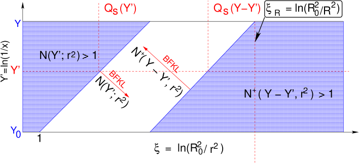
Figure 23: The kinematic region, where we can replace the non-linear system of equations given by Eq. (6.1) and Eq. (6.1) (see also Eq. (6.229) and Eq. (6.230)), by the linear BFKL equation.$R$ and $R_{0}$ are the sizes of projectile and target dipoles, $R\,\ll\,R_{0}$).

These sizes are to the right of the left line in Fig. 23. For $Q_{s}(Y-Y^{\prime})$ we have a different normalization, namely $Q_{0}(Y-Y^{\prime}=Y_{0})=1/R^{2}$ and instead of Eq. (6.226) we have

$$\ln(r^{2}/R^{2})\,\geq\,\,\frac{\omega(\gamma_{cr})}{1-\gamma_{cr}}\,\,(Y-Y^{\prime}-Y_{0})\,\,\,\,\,\mbox{or}\,\,\,\,\,\ln(R^{2}_{0}/r^{2})\,\,\leq\,\,\ln(R^{2}_{0}/R^{2})\,\,\,-\,\,\frac{\omega(\gamma_{cr})}{1-\gamma_{cr}}\,\,(Y-Y^{\prime}-Y_{0})$$ (6.227)

Finally, the BFKL equation can describe the scattering amplitude in the band shown in Fig. 23 which has the form

$$\ln\left(R^{2}_{0}Q^{2}_{s}(Y-Y^{\prime})\right)\,\,\,\,\,\,\, \geq \,\,\,\,\,\ln(R^{2}_{0}/r^{2})\,\,\,\,\,\geq\,\,\,\,\,\,\,\,\,\,\,\ln\left(R^{2}_{0}Q^{2}_{s}(Y^{\prime})\right)\,\,\,\mbox{where}$$ (6.228)

$$\ln\left(R^{2}_{0}Q^{2}_{s}(Y-Y^{\prime})\right)\,\,\,\,\,\,\, = \,\,\,\,\,\ln(R^{2}_{0}/R^{2})\,\,\,-\,\,\frac{\omega(\gamma_{cr})}{1-\gamma_{cr}}\,\,(Y-Y^{\prime}-Y_{0})\,;\,$$ (6.229)

$$\ln\left(R^{2}_{0}Q^{2}_{s}(Y^{\prime})\right)\,\,\,\,\,\,\,\,\,\,\,\,\,\,\,\,\,\, = \,\,\,\,\,\,\,\frac{\omega(\gamma_{cr})}{1-\gamma_{cr}}\,\,(Y^{\prime}-Y_{0})\,;$$ (6.230)

This result has been derived by Mueller and Shoshi (see Ref. [24]) using quite a different approach based on the completeness relation for the dipole number density (or in other words, a unitarity constraints in $t$-channel). In this approach the same conclusions stem from the semi-classical equation for the scattering amplitude.

The most interesting result of Ref. [24] is the appearance of a new saturation scale which has the form

$$\ln\left(R^{2}_{0}\,\tilde{Q}^{2}_{s}(Y)\right)\,\,=\,\,\ln\left(R^{2}_{0}\,Q^{2}_{s}(Y)\right)\,\,+\,\,c_{s}\frac{\pi^{2}\bar{\alpha}_{S}\,\chi^{{}^{\prime\prime}}_{\gamma,\gamma}(\gamma_{cr})(1-\gamma_{cr})^{2}}{8\,\ln^{3}(1/\bar{\alpha}_{S})}\,\,=\,\,\bar{\alpha}_{S}\,C_{s}\,Y$$ (6.231)

where $c_{s}$ is a constant which is determined by the exact value of the amplitude where the saturation is declared to occur. Constant $C_{s}$ is equal to

$$C_{s}\,\,\,\equiv\,\,\frac{\chi(\gamma_{cr})}{1-\gamma_{cr}}\,\,+\,\,\,c_{s}\frac{\pi^{2}\,\chi^{{}^{\prime\prime}}_{\gamma,\gamma}(\gamma_{cr})(1-\gamma_{cr})^{2}}{8\,\ln^{3}(1/\bar{\alpha}_{S})}$$ (6.232)

6.3 Solution in the saturation region

In the system of Eq. (6.1) and Eq. (6.1) we have used the relation of Eq. (2.29). However, we need to return to the general form of the action (see Eq. (2.20)) and to a general form of Eq. (6.1) and Eq. (6.1). This general form can be written as follows

$$\frac{\partial N(x,y;Y^{\prime})}{\partial\,Y^{\prime}}\,\,=$$

$$= \,\,\frac{\bar{\alpha}_{S}}{2\pi}\,\int\,d^{2}\,z\,K\left(x,y|z\right)\,\left(N(x,z;Y^{\prime})\,+\,N(z,y;Y^{\prime})\,-\,N(x,y;Y^{\prime})\,-N(z,y;Y^{\prime})\,N(z,y;Y^{\prime})\right)$$

$$- \,\frac{1}{(2\pi)^{4}}\,\frac{\bar{\alpha}_{S}}{\pi}\,\int\,\,G_{0}\left(x,y;Y^{\prime}|x^{\prime},y^{\prime};Y^{\prime}\right)\,\frac{d^{2}x^{\prime}\,d^{2}\,y^{\prime}}{(x^{\prime}-y^{\prime})^{4}}\,K\left(x^{\prime},y^{\prime}|z\right)\,\,d^{2}\,z\,\left(L_{z,y^{\prime}}\,N^{+}\left(z,y^{\prime},Y-Y^{\prime}\right)\right)\,N(x^{\prime},z;Y^{\prime})\,$$

$$\frac{\partial N^{+}(x,y;Y-Y^{\prime})}{\partial\,Y^{\prime}}\,\,=\,\,$$

$$= \,\,\frac{\bar{\alpha}_{S}}{2\pi}\,\int\,d^{2}\,z\,K\left(x,y|z\right)\,\left(N^{+}(x,z;Y-Y^{\prime})\,+\,N^{+}(z,y;Y-Y^{\prime})\,-\,N^{+}(x,y;Y-Y^{\prime})\,-\right.$$

$$- \left.\,\,N^{+}(z,y;Y-Y^{\prime})\,N^{+}(z,y;Y-Y^{\prime})\right)$$

$$- \,\,\frac{1}{(2\pi)^{4}}\,\frac{\bar{\alpha}_{S}}{\pi}\,\int\,\,G_{0}\left(x,y;Y^{\prime}|x^{\prime},y^{\prime};Y^{\prime}\right)\,\frac{d^{2}x^{\prime}\,d^{2}\,y^{\prime}}{(x^{\prime}-y^{\prime})^{4}}\,K\left(x^{\prime},y^{\prime}|z\right)\,\,d^{2}\,z\,\left(L_{z,y^{\prime}}N\left(z,y^{\prime};Y^{\prime}\right)\right)\,N^{+}(x^{\prime},z;Y-Y^{\prime})\,$$

One can see that in the kinematic region where (see Fig. 24)

$$\frac{r^{2}}{R^{2}_{0}}\,Q^{2}_{s}(Y^{\prime})\,\,<\,\,1\,;\,\,\,\,\,\,\,\,\,\,\,\,\,\,\,\,\,\,\mbox{and}\,\,\,\,\,\,\,\,\,\,\,\,\,\,\,\,\,\,\frac{R^{2}}{r^{2}}\,Q^{2}_{s}(Y-Y^{\prime})\,\,<\,\,1$$ (6.235)

both amplitudes $N\left(r,R_{0};Y^{\prime}\right)$ and $N\left(R,r;Y-Y^{\prime}\right)$ are deeply in the saturation region. We can find the solution of Eq. (6.3) and Eq. (6.3) in this region replacing both $N$ by $N=1+\Delta N$ and noticing that constant $N^{+}$ in Eq. (6.3), as well as constant $N$ in Eq. (6.3), does not give a contribution we see that the asymptotic solution is $N=1$ and for $\Delta N$ we have the following equation

$$\frac{\partial\left(L_{x,y}\Delta N(x,y;Y^{\prime})\right)}{\partial\,Y^{\prime}}\,\,=$$ (6.236)

$$\,\,-\frac{\bar{\alpha}_{S}}{2\pi}\,\int\,d^{2}\,z\,K\left(x,y|z\right)\,\left(L_{x,y}\Delta N(x,y;Y^{\prime})\right)\,\,-\,\,\frac{\bar{\alpha}_{S}}{2\pi}\,\int\,d^{2}\,z\,K\left(x,y|z\right)\left(L_{x,z}\Delta N(x,z;Y^{\prime})\right)$$

In Eq. (6.236) we neglect all contributions of the order $(\Delta N)^{2}$, $\Delta N\,\Delta N^{+}$ and $(\Delta N^{+})^{2}$.

Eq. (6.236) has a solution if we assume that $\Delta N$ has a geometrical scaling [50], namely, $\Delta N$ is a function of one variable

$$\zeta\,\,\,=\,\,\,\ln\left(\frac{r^{2}}{R^{2}_{0}}\,\tilde{Q}^{2}_{s}(Y^{\prime})\right)\,\,=\,\,\xi\,\,-\,\,\ln\left(R^{2}_{0}\,\tilde{Q}^{2}_{s}(Y^{\prime})\right)$$ (6.237)

where $\tilde{Q}_{s}$ is given by Eq. (6.231).

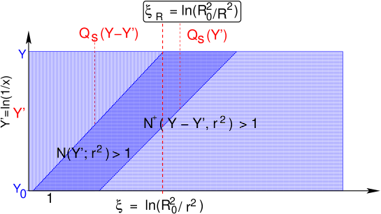
Figure 24: The kinematic region where both amplitudes $N(r^{2},R^{2}_{0};Y^{\prime})$ and $N(r^{2},R^{2};Y-Y^{\prime})$ are in the saturation region.

Using Eq. (6.222) we can rewrite Eq. (6.236) in the form

$$C_{s}\frac{\Delta\tilde{N}(\zeta)}{d\zeta}\,\,=\,\,-\,\,\zeta\,\Delta\tilde{N}(\zeta)\,\,-\,\,\int_{1/\tilde{Q}_{s}(Y^{\prime})}\,\frac{d^{2}z}{\pi}\,K(x,y;z)\,\,\Delta\tilde{N}(x,z;Y^{\prime})$$ (6.238)

where $\tilde{N}\,\,=\,\,L_{x,y}N(x,y;Y)$. In Ref. [50] it is shown that the main contribution in the saturation region stems from logarithmic integration, namely,

$$\int_{1/\tilde{Q}_{s}(Y^{\prime})}\,\,\frac{d^{2}z}{\pi}\,\,K(x,y;z)\,\,\,\,\longrightarrow\,\,\,\,\int^{(x-y)^{2}}_{1/\tilde{Q}_{s}(Y^{\prime})}\,\,\frac{dz^{2}}{(x-z)^{2}}\,\,\,\,+\,\,\,\,\int^{(x-y)^{2}}_{1/\tilde{Q}_{s}(Y^{\prime})}\,\,\frac{dz^{2}}{(y-z)^{2}}$$ (6.239)

Eq. (6.239) reduces Eq. (6.238) to

$$C_{s}\,\frac{\Delta\tilde{N}(\zeta)}{d\zeta}\,\,=\,\,-\,\,2\,\,\zeta\,\Delta\tilde{N}(\zeta)\,\,-\,\int^{\zeta}\,d\zeta^{\prime}\Delta\tilde{N}(\zeta^{\prime})$$ (6.240)

Introducing a new function $\Delta{\cal N}(\zeta)\,\,=\,\,\int^{\zeta}\,d\zeta^{\prime}\Delta\tilde{N}(\zeta^{\prime})$ we can rewrite Eq. (6.240) in the form

$$C_{s}\,\Delta{\cal N}"_{\zeta,\zeta}\,\,=\,\,-\,\,2\,\,\zeta\,\Delta{\cal N}"_{\zeta}(\zeta)\,\,-\,\,\Delta{\cal N}$$ (6.241)

the solution of this equation is equal to (see 9.255(2) in Ref. [48]

$$\Delta{\cal N}(\zeta)\,\,=\,\,\exp\left\{-\frac{\zeta^{2}}{2\,C_{s}}\,\right\}\,D_{-\frac{1}{2}}\left(\sqrt{\frac{2}{C_{s}}}\,\zeta\right)$$ (6.242)

where $D_{p}(t)$ is the parabolic cylinder function (see 9.240 - 9.255 in Ref. [48]). Eq. (6.242) leads to

$$\Delta{\cal N}(\zeta)\,\,\,\longrightarrow\,\,\exp\left(-\frac{\zeta^{2}}{C_{s}}\right)$$ (6.243)

In semi-classical approach Eq. (6.243) leads to $\Delta N\,\propto\,\exp\left(-\,\frac{1-\gamma_{cr}}{\omega(\gamma_{cr})}\,\zeta^{2}\right)$ in the case if we neglect the difference between $Q_{s}$ and $\tilde{Q}_{s}$ (see Eq. (6.231). This result is very surprising. Indeed, the approach to the asymptotic solution in the case of the Balitsky-Kovchegov equation gives $\Delta N\propto\,exp\left(-\,\frac{1-\gamma_{cr}}{2\,\omega(\gamma_{cr})}\,\zeta^{2}\right)$ [50] which is slower than Eq. (6.243). The estimates based on the Iancu - Mueller approach [15, 16] gave even smaller coefficient in the exponent than for the Balitsky-Kovchegov equation. The solution of the functional equation (see previous section and Ref. [21]) also gives a coefficient which is in two times smaller than in the Iancu - Mueller approach. In the last two approaches the $t$-channel unitarity has been heavily used. Certainly, the BFKL Pomeron Calculus satisfies the $t$-channel unitarity constraints, but we cannot guarantee that the semi-classical approach respects $t$ - channel unitarity.

The second problem with the solution of Eq. (6.243) could be our assumption that the solution in the saturation region has the same geometrical scaling behaviour as the solution to the Balitsky-Kovchegov equation. In Ref. [24] it is shown that the geometrical scaling is not correct assumption in the vicinity of the saturation scale in the Mueller-Shoshi band. What happens inside the saturation region we have not studied yet. To find out whether the geometrical scaling behaviour is an inherent property of the system we need to solve Eq. (6.1) and Eq. (6.1) in the vicinity of two saturation scales taking into account the non-linear corrections. We will do this in further publications.

7 Conclusions

We show in this paper that the BFKL Pomeron Calculus in the kinematic region given by Eq. (1.3) has two equivalent descriptions: (i)  one is the generating functional which gives a clear probabilistic interpretation of the processes of high energy scattering and provides also a Hamiltotian-like description of the system of interacting dipoles; (ii)  the second is the Langevin equation for directed percolation (see Eq. (3.60)). We are able to prove this equation for the dipoles in the momentum represetation if the impact parametrepresentationlarger than $b\,\gg 1/k$ where $k$ is the transverse momentum of a dipole.

In other words, the BFKL Pomeron Calculus can be considered as an alternative description of the statistical system of dipoles with different kinds of interactions between them.

One of the results of this paper is the understanding the two Pomerons to one Pomeron merging in the framework of the dipole approach. It turns out that the Feynman diagrams of Fig. 18, Fig. 19 and Fig. 20 describe the process given by Eq. (4.155). In this process two dipoles are produced in the first stage and two other dipoles in the second stage of the processes. All these four dipoles can interact with the target leading to Eq. (4.159) for the contribution to the generating functional. At first sight, Eq. (4.159) contradicts the probabilistic treatment due to the negative sign in front of this term in Eq. (3.69). Indeed, it seems strange that two dipoles decay into four dipoles with negative amplitude since this amplitude looks rather as probability of this decay. We showed in section 4 that this sign minus has a very simple explanation and stems from the fact that the decay of two dipoles into four actually goes in two stages. During the first one, one dipole decays into two with positive probability. During the second stage of the process the second dipole scatters off the produced two dipoles. This rescattering does not produce the new dipoles but change the two dipoles, produced during the first stage, to two new dipoles. This rescattering process goes in the Born approximation of perturbative QCD but it generates almost a pure imaginary scattering amplitude. This fact results in extra minus sign. The calculations of section 4 suggest the educated guess: all processes of merging for Pomerons ( say $nP\to mP$ with $m<n$, for example such as $3P\to 2P$) will lead to the term in Eq. (3.69) and Eq. (3.71) of the following type:

$$\prod_{i}^{2n}u(x_{i},y_{i})\,\prod^{n}_{l}\frac{\delta}{\delta u(x_{l},y_{l})}$$ (7.244)

It should be stressed that the vertex in front of Eq. (7.244) can be found directly from the JIMWLK approach as [37] as it was demonstrated in Ref. [45]. Therefore, the evolution equations (Markov’s chain) for the generating functional together with the JIMWLK approach lead to the selfconsistent and complete theory of high energy interaction in QCD.

It should be stressed that the negative sign does not change the fact that the high energy amplitude can be written in terms of probabilities to find the given number of dipoles of definite sizes (see Eq. (3.65)). It was shown in section 3.3 that the equations for generating functional can be rewritten as the path integral for the partition function using which we can introduce the thermodynamic potential to describe the system of dipoles.

It is shown that the question about negative amplitude does not arise if we treat the system of dipoles in the momentum representation. Markov’s chain of equation for this system is written in the paper (see Eq. (4.195)) and can be considered as a practical way to find a solution in accessible range of energies.

The result of this paper is the solution to the linear functional equation for the generating functional in the high energy region. We found the semi-classical solution for the toy model in the entire kinematic region while we were able to calculate the asymptotic solution and the first correction to it at high energy in the general case of interacting dipoles. This solution shows the two BFKL Pomerons to one BFKL Pomeron merging is essential only in the limited region of the phase space where the resulting vertex is positive.

The third result of this paper is the first attempt to solve the semi-classical equations for the BFKL Pomeron calculus. We confirm the Mueller-Shoshi band in $\ln(1/x)$ and $\xi=\ln(R^{2}_{0}/r^{2})$ plane where the solution to the linear BFKL equation can describe the scattering amplitude which follows from the set of equation in the semi-classical approach. We found the solution deeply in the saturation region where the scattering amplitude approaches unity ($N\,\rightarrow\,1$). It turns out that approach is steeper for our case than for the mean field approximation.

Being elegant and beautiful the BFKL Pomeron Calculus has a clear disadvantage: it lacks theoretical ideas what kind of Pomeron interactions we should take into account and why. Of course, the Feynman diagrams in leading $\ln(1/x)$ approximation of perturbative QCD allow us, in principle, to calculate all possible Pomeron interactions but, practically, it is very hard job. Even if we calculate these vertices we need to understand what set of vertices we should take into account for calculation of the scattering amplitude. In this paper we show that the the BFKL Pomeron calculus together with the JIMWLK approach allows us to build the selfconsistent and complete theory of the high energy scattering in QCD. However, we lack the formalism how to extract the multi Pomeron vertices from the JIMWLK approach as well as the general approach which will allow us to take into account all possible multi Pomeron vertices. This is the reason why we need to develop a more general formalism. Fortunately, such a formalism has been built and it is known under the abbreviation JIMWLK-Balitsky approach [40, 37, 28]. In this approach we are able to calculate all vertices for Pomeron interactions as it was demonstrated in Ref. [45] and it solves the first part of the problem: determination of all possible Pomeron interactions. However, we need to understand what vertices we should take into account for calculation of the scattering amplitude. We hope that a further progress in going beyond of the BFKL Pomeron Calculus (see Refs. [45, 46]) will lead to such a development of the BFKL Pomeron Calculus that we will have a consistent theoretical approach. Hopefully this approach will be simpler than Lipatov’s effective action [47] which is not easier to solve than the full QCD Lagrangian.

It is well known that the mean field approach to our problem which includes only one dipole to two dipoles decay in the master equation (see Eq. (3.69)) has been studied quite well both analytically [50] and numerically [52]. We firmly believe that the probabilistic interpretation gives a practical method for creating a Monte Carlo code in spirit of the approach suggested in Ref. [53]. This code will allow us to find a numerical solution to the problem and to consider the inclusive observables. This extension is very desirable since the most experimental data exist for these observables. We also hope that the semi-classical approach for searching the solution to the master equation will be useful for developing both analytical and numerical approaches which will result in predictions for the LHC.

Appendix A Calculation of $G_{0}(x_{1},x_{2}|x^{\prime}_{1},x^{\prime}_{2})$.

The solution of the BFKL equation is given by [26]

$$G(x_{1},x_{2};x^{{}^{\prime}}_{1},x^{{}^{\prime}}_{2}|\omega)\,=\,\sum_{n=-\infty}^{+\infty}\int_{-\infty}^{+\infty}\frac{(\nu^{2}+n^{2}/4)d\nu}{[\nu^{2}+(n-1)^{2}/4][\nu^{2}+(n+1)^{2}/4]}\frac{G_{\nu\mu}(x_{1},x_{2},x^{{}^{\prime}}_{1},x^{{}^{\prime}}_{2})}{\omega-\omega(\nu,\mu)}$$ (A.245)

where $G_{\nu\mu}(x_{1},x_{2},x^{{}^{\prime}}_{1},x^{{}^{\prime}}_{2})$ is the Mellin transform of Eq. (2.11) and $x_{i}$ are two-dimensional vectors in complex coordinates

$$x_{i}=x_{i,x}+ix_{i,y} x^{*}_{i}=x_{i,x}-ix_{i,y}$$ (A.246)

The function $\omega(\nu,\mu)$ is the eigen value of the BFKL equation given by Eq. (2.13).

The four-point Green function is presented in terms of the hypergeometric functions [26, 6]

$$G_{\nu\mu}(x_{1},x_{2},x^{{}^{\prime}}_{1},x^{{}^{\prime}}_{2})=C_{1}x^{h}x^{*\tilde{h}}F(h,h,2h;x)F(\tilde{h},\tilde{h},2\tilde{h};x^{*})$$

$$+C_{2}x^{1-h}x^{*1-\tilde{h}}F(1-h,1-h,2-2h;x)F(1-\tilde{h},1-\tilde{h},2-2\tilde{h};x^{*})$$ (A.247)

with $h=\frac{1}{2}+i\nu+\frac{n}{2}$, $\tilde{h}=\frac{1}{2}+i\nu-\frac{n}{2}$, and $x$ is the anharmonic ratio

$$x=\frac{x_{12}x_{1^{\prime}2^{\prime}}}{x_{11^{\prime}}x_{22^{\prime}}}$$ (A.248)

Coefficients $C_{1}$ and $C_{2}$ are given by [26]

$$C_{1}=\frac{b_{n,-\nu}}{2\pi^{2}}\hskip 56.9055ptC_{2}=\frac{b_{n,\nu}}{2\pi^{2}}$$ (A.249)

with

$$b_{n,\nu}=\pi^{3}2^{4i\nu}\frac{\Gamma(-i\nu+(1+|n|)/2)\Gamma(i\nu+|n|/2)}{\Gamma(i\nu+(1+|n|)/2)\Gamma(-i\nu+|n|/2)}$$ (A.250)

As we have discussed, the high energy asymptotic behaviour stems from $n=0$ term in Eq. (A.245). The initial condition for Eq. (2.11) at $Y=Y_{0}$ is given by the following expression

$$G_{0}(x_{1},x_{2};x^{\prime}_{1},x^{\prime}_{2})\,\,=$$ (A.251)

$$\,\,\int\,\frac{d\omega}{2\,\pi\,i}\int_{-\infty}^{+\infty}\,\,\frac{\nu^{2}d\nu}{(\nu^{2}+1/4)^{2}}\frac{G_{\nu\mu}(x_{1},x_{2},x^{\prime}_{1},x^{\prime}_{2})}{\omega-\omega(\nu,n=0)}\,=\,\frac{1}{\omega}\int_{-\infty}^{+\infty}\,\,\frac{\nu^{2}d\nu}{(\nu^{2}+1/4)^{2}}\,\,G_{\nu\mu}(x_{1},x_{2},x^{\prime}_{1},x^{\prime}_{2})$$

This integral can be taken by closing contour of integration over singularities of the integrand.

The function

$$\frac{\nu^{2}}{(\nu^{2}+1/4)^{2}}$$ (A.252)

has two poles at $\frac{i}{2}$ and $-\frac{i}{2}$. The four-point Green function of Eq. (A) consists of two terms, one with $C_{1}(xx^{*})^{\frac{1}{2}+i\nu}$ and the other one $C_{2}(xx^{*})^{\frac{1}{2}-i\nu}$. For small $|x|$ this terms should be integrated closing contour in upper and lower semi-planes respectively. The resulting contour in the lower semi-plane runs anticlockwise and thus the value of the contour integral enters with a minus sign.

The terms could be expanded in the vicinity of their poles. Let us consider the first term. We expand the function $C_{1}$ in the vicinity of $\frac{i}{2}$

$$C_{1}=\frac{\pi}{2}2^{-4i\nu}\frac{\Gamma(-i\nu)}{\Gamma(-i\nu+\frac{1}{2})\Gamma(1+i\nu)}\frac{\Gamma(i\nu+\frac{3}{2})}{(i\nu+\frac{1}{2})}$$ (A.253)

The hypergeometric function can be written as a sum

$$F(a,b,c;x)=1+\frac{\Gamma(c)}{\Gamma(a)\Gamma(b)}\sum^{\infty}_{n=1}\frac{\Gamma(a+n)\Gamma(b+n)}{\Gamma(c+n)}\frac{x^{n}}{n!}$$ (A.254)

In the case of $F(h,h,2h;x)$ the singularity of $\Gamma$ function at $\frac{i}{2}$ can factorized out the sum

$$F(h,h,2h;x)=1+\frac{\Gamma(2h)}{\Gamma(h)\Gamma(h)}\sum^{\infty}_{n=1}\frac{\Gamma(h+n)\Gamma(h+n)}{\Gamma(2h+n)}\frac{x^{n}}{n!}$$

$$\simeq 1+\frac{1}{2\Gamma(h)}\sum^{\infty}_{n=1}\frac{x^{n}}{n}=1-\frac{1}{2}\frac{ln(1-x)}{\Gamma(i\nu+\frac{1}{2})}$$ (A.255)

At this stage the first term of the integrand of Eq. (A.251) can be written as

(A.256)

$$\frac{1}{\omega}\frac{\nu^{2}}{(i\nu+\frac{1}{2})^{3}(i\nu-\frac{1}{2})^{2}}\frac{\pi}{2}2^{-4i\nu}\frac{\Gamma(-i\nu)}{\Gamma(-i\nu+\frac{1}{2})\Gamma(1+i\nu)}(xx^{*})^{\frac{1}{2}+i\nu}\left(1-\frac{1}{2}\frac{ln(1-x)}{\Gamma(\frac{1}{2}+i\nu)}\right)\left(1-\frac{1}{2}\frac{ln(1-x^{*})}{\Gamma(\frac{1}{2}+i\nu)}\right)$$

It is clearly seen that the term of zero order in $ln|1-x|$ has a third order pole at $\nu=\frac{i}{2}$; the term of first order in $ln|1-x|$ has a second order pole at $\nu=\frac{i}{2}$, and, the term of second order in $ln|1-x|$ has a simple pole at $\nu=\frac{i}{2}$. The contributions of those terms in the contour integral are found to be

$$\frac{i\pi^{2}}{\omega}[-2\,\,+\,\,ln(xx^{*})(-4+ln(xx^{*}))]$$ (A.257)

$$-\frac{\pi^{2}}{2\omega}[-2\,\,+\,\,\gamma\,\,+\,\,ln(xx^{*})]ln[(1-x)(1-x^{*})]$$ (A.258)

$$-\frac{i\pi^{2}}{4\omega}ln(1-x)ln(1-x^{*})$$ (A.259)

respectively.

In a similar way we may expand the second of the integrand in vicinity of its pole at $\nu=-\frac{i}{2}$, namely

(A.260)

$$\frac{1}{\omega}\frac{\nu^{2}}{(\frac{1}{2}-i\nu)^{3}(i\nu+\frac{1}{2})^{2}}\frac{\pi}{2}2^{4i\nu}\frac{\Gamma(i\nu)}{\Gamma(i\nu+\frac{1}{2})\Gamma(1-i\nu)}(xx^{*})^{\frac{1}{2}-i\nu}\left(1-\frac{1}{2}\frac{ln(1-x)}{\Gamma(\frac{1}{2}-i\nu)}\right)\left(1-\frac{1}{2}\frac{ln(1-x^{*})}{\Gamma(\frac{1}{2}-i\nu)}\right)$$

The integration is performed on the lower semicircle and results in overall minus sign of the integral. The contributions corresponding to Eq. (A.257), Eq. (A.258) and Eq. (A.259) are

$$-\frac{i\pi^{2}}{\omega}[-\,\,2\,\,+\,\,ln(xx^{*})(-4+ln(xx^{*}))]$$ (A.261)

$$-\frac{\pi^{2}}{2\omega}[-2\,\,+\,\,\gamma\,\,+\,\,ln(xx^{*})]ln[(1-x)(1-x^{*})]$$ (A.262)

$$+\frac{i\pi^{2}}{4\omega}ln(1-x)ln(1-x^{*})$$ (A.263)

respectively.

Comparing the contributions we note that that of zero and second order
in $ln[(1-x)(1-x^{*})]$ are exactly canceled out, and we are left with

$$-2\frac{\pi^{2}}{2\omega}[-2\,\,+\,\,\gamma\,\,+\,\,ln(xx^{*})]ln[(1-x)(1-x^{*})]$$ (A.264)

For small $|x|$ this can written as

$$-\frac{4\pi^{2}}{\omega}\hskip 4.26773ptln|x|\hskip 4.26773ptln|1-x|$$ (A.265)

or

$$+\frac{4\pi^{2}}{\omega}\hskip 4.26773ptln\frac{1}{|x|}\hskip 4.26773ptln|1-x|$$ (A.266)

Going back to complex vector representation of x and rewriting Eq. (A.267) as

$$G_{0}(x_{1},x_{2};x^{\prime}_{1},x^{\prime}_{2})\,\,=\,\,+\frac{4\pi^{2}}{\omega}\hskip 4.26773ptln\left|\frac{x_{11^{\prime}}x_{22^{\prime}}}{x_{12^{\prime}}x_{1^{\prime}2}}\right|\hskip 4.26773ptln\left|\frac{x_{11^{\prime}}x_{22^{\prime}}}{x_{12}x_{1^{\prime}2^{\prime}}}\right|$$ (A.267)

we see that we reproduce the result of [26]. Therefore, we demonstrated that Eq. (A.267) gives a correct initial condition for searching the scattering amplitude at high energies restricting ourselves by the one term in Eq. (2.11) with $n=0$.

Appendix B The path integral formalism for the generating functional.

We want to develop a path integral formalism similar to that we found for the toy model, but where the probabilities to find $n$ dipoles depend of dipole sizes. In our notation we denote by Latin index rapidity interval, and Greek indices relate to a size of dipole.

As in Chapter 3.3 we introduce the creation and annihilation operators

$$\hat{a}(q)=\frac{\delta}{\delta u(q)}\hskip 56.9055pt\hat{a}^{\dagger}(q)=u(q)$$ (B.268)

with commutation relations $[\hat{a}(q),\hat{a}^{\dagger}(q^{\prime})]=\delta(q-q^{\prime})$ at fixed $Y$. The expression for the coherent states in this case takes form of

$$|\phi(q)>=e^{\phi(q)\hat{a}^{\dagger}(q)-\phi(q)}|0>$$ (B.269)

with

$$\hat{a}(q^{\prime})|\phi(q)>=\phi(q)|\phi(q)>\delta(q-q^{\prime})$$ (B.270)

First we consider discrete dipole sizes $q_{\alpha}=(L/N)\alpha$, where $L$ is a maximal possible dipole size, $N$ a number of intervals of $L$ discretization, and $\alpha$ is an integer number running from $0$ to $N$. In this case the commutation relations become $[\hat{a}(q_{\alpha}),\hat{a}^{\dagger}(q_{\beta})]=\delta_{\alpha,\beta}$.

The unit operator can be written in terms of the coherent states

$$\hat{I}=\prod_{\alpha}\int\frac{d\phi^{*}(q_{\alpha})d\phi(q_{\alpha})}{i\pi}e^{-\phi^{*}(q_{\alpha})\phi(q_{\alpha})+\phi(q_{\alpha})+\phi^{*}(q_{\alpha})}|\phi(q_{\alpha})><\phi(q_{\alpha})|$$ (B.271)

The operator $\mathcal{H}$ defined in Eq. (3.71) can be written as

$$\mathcal{H}[\hat{a}^{\dagger},\hat{a}]= - \sum_{\beta}\sum_{\gamma}\sum_{\lambda}[V_{1\rightarrow 2}(q_{\beta}\rightarrow q_{\gamma}+q_{\lambda})\{-\hat{a}^{\dagger}(q_{\beta})+\hat{a}^{\dagger}(q_{\gamma})\hat{a}^{\dagger}(q_{\lambda})\}\hat{a}(q_{\beta})$$ (B.272)

$$- V_{2\rightarrow 1}(q_{\gamma}+q_{\lambda}\rightarrow q_{\beta})\{\hat{a}^{\dagger}(q_{\gamma})\hat{a}^{\dagger}(q_{\lambda})-\hat{a}^{\dagger}(q_{\beta})\}\frac{1}{2}\hat{a}(q_{\gamma})\hat{a}(q_{\lambda})]$$

Following the logic of Chapter 3.3 we consider a matrix element

$$\left\{\prod_{\alpha^{\prime}}<\phi_{j+1}(q_{\alpha^{\prime}})|\right\}(1+\mathcal{H}\Delta Y)\left\{|\prod_{\alpha}\phi_{j}(q_{\alpha})>\right\}$$ (B.273)

First, look at the second term of the Hamiltonian

$$\left\{\prod_{\alpha^{\prime}}<\phi_{j+1}(q_{\alpha^{\prime}})|\right\}\sum_{\beta}\sum_{\gamma}\sum_{\lambda}[-V_{1\rightarrow 2}(q_{\beta}\rightarrow q_{\gamma}+q_{\lambda})\hat{a}^{\dagger}(q_{\gamma})\hat{a}^{\dagger}(q_{\lambda})\hat{a}(q_{\beta})]\left\{\prod_{\alpha}|\phi_{j}(q_{\alpha})>\right\}$$

$$\left\{\prod_{\alpha^{\prime}}<\phi_{j+1}(q_{\alpha^{\prime}})|\right\}\sum_{\beta}\sum_{\gamma}\sum_{\lambda}[-V_{1\rightarrow 2}(q_{\beta}\rightarrow q_{\gamma}+q_{\lambda})\phi^{*}_{j+1}(q_{\gamma})\phi^{*}_{j+1}(q_{\lambda})\phi_{j}(q_{\beta})]\left\{\prod_{\alpha}|\phi_{j}(q_{\alpha})>\right\}$$ (B.274)

In Eq. (B) we used the property of the coherent states given by Eq. (B.270).

In the continuous limit $\delta_{\alpha,\beta}$ is replaced by $\delta(q_{\alpha}-q_{\beta})$, and $\prod_{\alpha}d\phi^{*}(q_{\alpha})d\phi(q_{\alpha})$ by functional integration $\int\mathcal{D}\phi^{*}\mathcal{D}\phi$.

From here we see that rest of the calculations is similar to that of Chapter 3.3 and we end up with the expression for a matrix element of an operator $A$ between states of initial $Y_{0}$ and final rapidity $Y$

$$<Y|A|Y_{0}>\sim\int\mathcal{D}\Phi^{+}\mathcal{D}\Phi A(Y)e^{S}$$ (B.275)

where

$$S\, = \,\int\left(\int\Phi^{+}(q)\frac{d}{dY}\Phi(q)dq+\mathcal{H}(\Phi^{+}+1,-\Phi)\,\right)dY$$ (B.276)

with the Hamiltonian given by

$$\mathcal{H} =$$ (B.277)

$$+ \int d^{4}q_{0}d^{4}q_{1}d^{4}q_{2}[V_{1\rightarrow 2}(q_{0}\rightarrow q_{1}+q_{2})\{-\Phi^{+}(q_{0})+\Phi^{+}(q_{1})+\Phi^{+}(q_{2})+\Phi^{+}(q_{1})\Phi^{+}(q_{2})\}\Phi(q_{0})$$

$$- V_{2\rightarrow 1}(q_{1}+q_{2}\rightarrow q_{0})\{\Phi^{+}(q_{1})\Phi^{+}(q_{2})+\Phi^{+}(q_{1})+\Phi^{+}(q_{2})-\Phi^{+}(q_{0})\}\frac{1}{2}\Phi(q_{1})\Phi(q_{2})]$$

Appendix C The exact calculations in the semi-classical approach

At this appendix we calculate exactly exponent in semi-classical solution and compare it with it approximations at small and large values of $\omega$, which ware used for calculation of corresponding weight functions.

Remind that Eq. (4.171)

$$\Phi^{\pm}_{u}\,\,=\,\,\frac{\kappa_{1}}{2\,\,L(u)}\,\left\{\,\,1\,\,\pm\,\,\sqrt{1\,\,+\,\,\frac{4\,\,\omega\,\,L(u)}{\,\,\kappa_{1}\,\,u\,(1-u)\,}}\,\,\right\}$$ (C.278)

Therefore exponent in semi-classical solution $\Phi^{\pm}$ will be defined by the following integrals:

$$\Phi^{\pm}(u)\,\,=\,\,\int_{0}^{u}\frac{\kappa_{1}}{2\,\,L(u^{\prime})}\,\left\{\,\,1\,\,\pm\,\,\sqrt{1\,\,+\,\,\frac{4\,\,\omega\,\,L(u^{\prime})}{\,\,\kappa_{1}\,\,u^{\prime}\,(1-u^{\prime})\,}}\,\,\right\}\,du^{\prime}\,=\,I_{1}\,+\,I_{2}$$ (C.279)

where

$$I_{1}\, = \,\,\int_{0}^{u}\frac{\kappa_{1}}{2\,\,L(u^{\prime})}\,du^{\prime}$$

$$= \,\,\frac{2}{\sqrt{6\kappa_{2}-1-\kappa_{2}^{2}}}\cdot\left[\arctan\left(\frac{1-\kappa_{2}+2u}{\sqrt{6\kappa_{2}-1-\kappa_{2}^{2}}}\right)\,-\,\arctan\left(\frac{1-\kappa_{2}}{\sqrt{6\kappa_{2}-1-\kappa_{2}^{2}}}\right)\right]$$

$$I_{2}\,\, = \,\,\pm\,\frac{\kappa_{1}}{2}\int_{0}^{u}\,\frac{du^{\prime}}{L(u^{\prime})}\,\sqrt{1\,\,+\,\,\frac{4\,\,\omega\,\,L(u^{\prime})}{\,\,\kappa_{1}\,\,u^{\prime}\,(1-u^{\prime})\,}}$$ (C.281)

$$= \,\,\pm\,\frac{\kappa_{1}}{2}\int_{0}^{u}\,\frac{du^{\prime}}{u^{\prime}(1+u^{\prime})+\kappa_{2}(1-u^{\prime})}\,\sqrt{1\,\,+\,\,\frac{4\,\,\omega\cdot[u^{\prime}(1+u^{\prime})+\kappa_{2}(1-u^{\prime})]}{\,\,\kappa_{1}\,\,u^{\prime}\,(1-u^{\prime})\,}}$$

$$= \,\,\pm\,\,[\,II_{2}(u)-II_{2}(0)\,]$$

where $II_{2}$ defined as following indefinite integral:

$$II_{2}(t)\,\, = \,t\,\,\sqrt{-\,\,\frac{(A^{+}\,+\,8\omega\frac{\kappa_{2}}{\kappa_{1}}(1-t))\cdot(A^{-}\,+\,8\omega\frac{\kappa_{2}}{\kappa_{1}}(1-t))}{4^{3}\omega^{2}\frac{\kappa_{2}}{\kappa_{1}^{2}}}}\,\,\sqrt{1+4\omega\,\frac{\frac{\kappa_{2}}{\kappa_{1}}+\frac{1-\kappa_{2}}{\kappa_{1}}t+\kappa_{2}t^{2}}{t(1-t)}}$$

$$\,\cdot\{\left(4\omega\sqrt{\frac{1}{\kappa_{1}^{2}}-6\frac{\kappa_{2}}{\kappa_{1}^{2}}+\frac{\kappa_{2}^{2}}{\kappa_{1}^{2}}}\right)EF\left[i\cdot\arcsin h\left(\sqrt{\frac{4\omega}{A^{-}}\cdot\frac{\kappa_{2}}{\kappa_{1}}\cdot\frac{t}{1-t}}\right),\,\,\frac{A^{-}}{A^{+}}\right]$$

$$-\,EPi\left[-\,\frac{A^{-}}{\frac{4\omega}{\kappa_{1}}\cdot(-1-\kappa_{2}+\sqrt{1-6\kappa_{2}+\kappa_{2}^{2}})},\,\,i\cdot\arcsin h\left(\sqrt{\frac{8\omega}{A^{-}}\cdot\frac{\kappa_{2}}{\kappa_{1}}\cdot\frac{1-t}{t}}\right),\,\,\frac{A^{-}}{A^{+}}\right]$$

$$+\,EPi\left[\frac{A^{-}}{\frac{4\omega}{\kappa_{1}}\cdot(1+\kappa_{2}+\sqrt{1-6\kappa_{2}+\kappa_{2}^{2}})},\,\,i\cdot\arcsin h\left(\sqrt{\frac{8\omega}{A^{-}}\cdot\frac{\kappa_{2}}{\kappa_{1}}\cdot\frac{1-t}{t}}\right),\,\,\frac{A^{-}}{A^{+}}\right]\}$$

$$\cdot\frac{1}{\left[-t(1-t)-4\omega\,\frac{\frac{\kappa_{2}}{\kappa_{1}}+\frac{1-\kappa_{2}}{\kappa_{1}}t+\kappa_{2}t^{2}}{t(1-t)}\right]\cdot\sqrt{1-6\kappa_{2}+\kappa_{2}^{2}}\,\,\,\sqrt{\frac{4\omega}{A^{-}}\cdot\frac{\kappa_{2}}{\kappa_{1}}\cdot\frac{t}{1-t}}}$$

In the last relation we used the following notations:

$$A^{\pm} \equiv 1+\frac{4\omega}{\kappa_{1}}+4\omega\frac{\kappa_{2}}{\kappa_{1}}\;\pm\;\sqrt{-128\omega\frac{\kappa_{2}}{\kappa_{1}^{2}}+\left(1+\frac{4\omega}{\kappa_{1}}+4\omega\frac{\kappa_{2}}{\kappa_{1}}\right)^{2}}$$

$$EF(\varphi,m) \equiv \int_{0}^{\varphi}\frac{d\theta}{\sqrt{1-m\cdot\sin^{2}(\theta)}}\;=\;Elliptic\;integral\;of\;the\;first\;kind$$

$$EPi(n,\varphi,m) \equiv \int_{0}^{\varphi}\frac{d\theta}{(1-n\cdot\sin^{2}(\theta))\cdot\sqrt{1-m\cdot\sin^{2}(\theta)}}\;=\;Elliptic\;integral\;of\;the\;third\;kind$$

We can see that in spite the fact that $\Phi^{\pm}$ can be calculated explicitly (in radicals), it is too complicated in order to use it for the calculations of the weight functions $\phi^{\pm}(\omega)$ in Eq. (4.173) and Eq. (4.174). Nevertheless, this exact calculation very fruitful for two purposes: (I) using exact form of $\Phi^{\pm}$ we can estimate how good our approach for small and large $\omega$ (or in another words how good we estimated spectrum of our solution), (II) once we know our spectral functions $\phi^{\pm}(\omega)$ we can use this exact solution for the following calculations. It is important to note that $II_{2}(t)$ looks as imaginary functions, but on fact the imaginary part is closely related to regularization of singularity at $u=0$, thus it is essential in some since. The plots below illustrates how good our approach for small and large $\omega$, which we used for calculations of $\Phi^{\pm}$.

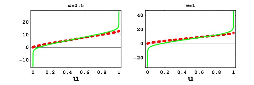
Figure 25: At this plot we compare positive branch of our exact result (thick doted line) with for $\phi(\omega)$ with approximation for small values of $\omega$ (i.e. $\omega>\frac{\kappa_{1}}{\kappa_{2}}$), which was used in Eq. (4.173)  (thin solid line)

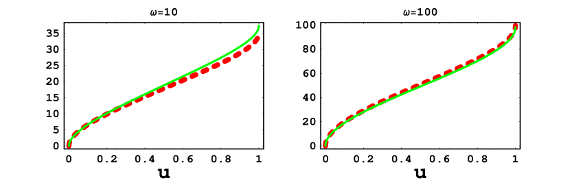
Figure 26: At this plot we compare positive branch of our exact result (thick doted line) with for $\phi(\omega)$ with approximation for large values of $\omega$ (i.e. $\omega>\frac{\kappa_{1}}{\kappa_{2}}$), which was used in Eq. (4.176)  (thin solid line)

References

- [1] L. V. Gribov, E. M. Levin and M. G. Ryskin, Phys. Rep. 100, 1 (1983).
- [2] A. H. Mueller and J. Qiu, Nucl. Phys.,427 B 268 (1986) .
- [3] E. A. Kuraev, L. N. Lipatov, and F. S. Fadin, Sov. Phys. JETP 45, 199 (1977); Ya. Ya. Balitsky and L. N. Lipatov, Sov. J. Nucl. Phys. 28, 22 (1978).
- [4] J. Bartels, M. Braun and G. P. Vacca, Eur. Phys. J. C40, 419 (2005) [arXiv:hep-ph/0412218] ; J. Bartels and C. Ewerz, JHEP 9909, 026 (1999) [arXiv:hep-ph/9908454] ; J. Bartels and M. Wusthoff, Z. Phys. C66, 157 (1995) ; A. H. Mueller and B. Patel, Nucl. Phys. B425, 471 (1994) [arXiv:hep-ph/9403256]; J. Bartels, Z. Phys. C60, 471 (1993).
- [5] M. A. Braun, Phys. Lett. B632 (2006) 297 [arXiv:hep-ph/0512057]; arXiv:hep-ph/0504002 ; Eur. Phys. J. C16, 337 (2000) [arXiv:hep-ph/0001268]; M. Braun, Eur. Phys. J. C6, 321 (1999) [arXiv:hep-ph/9706373]; M. A. Braun and G. P. Vacca, Eur. Phys. J. C6, 147 (1999) [arXiv:hep-ph/9711486].
- [6] H. Navelet and R. Peschanski, Nucl. Phys. B634, 291 (2002) [arXiv:hep-ph/0201285]; Phys. Rev. Lett. 82, 137 (1999), [arXiv:hep-ph/9809474]; Nucl. Phys. B507, 353 (1997) [arXiv:hep-ph/9703238].
- [7] J. Bartels, L. N. Lipatov and G. P. Vacca, Nucl. Phys. B706, 391 (2005) [arXiv:hep-ph/0404110].
- [8] V. N. Gribov, Sov. Phys. JETP 26, 414 (1968) [Zh. Eksp. Teor. Fiz. 53, 654 (1967)].
- [9] O.V. Kancheli, Sov. JETP Lett. 18, 274 (1973), in Caneschi, L. (ed.): “Regge theory of low-p(T) hadronic interactions’, p. 312, North-Holland, 1989; Pisma Zh. Eksp. Teor. Fiz. 22 (1975) 491.
- [10] P. Grassberger and K. Sundermeyer, Phys. Lett. B77, 220 (1978).
- [11] E. Levin, Phys. Rev. D49, 4469 (1994).
- [12] K. G. Boreskov, “Probabilistic model of Reggeon field theory,” arXiv:hep-ph/0112325 and reference therein.
- [13] C.W. Gardiner,“Handbook of Stochastic Methods for Physics, Chemistry and the Natural Science”, Springer-Verlag, Berlin, Heidelberg 1985.
-
[14]
G. Veneziano, Phys. Letters 52B (1974) 220; Nucl.
Phys.B74 (1974) 365;
M. Ciafaloni, G. Marchesini anf G. Veneziano, Nucl. Phys. B98 (1975) 493. - [15] E. Iancu and A. H. Mueller, Nucl. Phys. A730 (2004) 460, 494, [arXiv:hep-ph/0308315],[arXiv:hep-ph/0309276].
- [16] M. Kozlov and E. Levin, Nucl. Phys. A739 (2004) 291 [arXiv:hep-ph/0401118].
- [17] A. H. Mueller, Nucl. Phys. B415, 373 (1994); ibid B437, 107 (1995).
- [18] E. Levin and M. Lublinsky, Nucl. Phys. A730, 191 (2004) [arXiv:hep-ph/0308279].
- [19] E. Levin and M. Lublinsky, Phys. Lett. B607, 131 (2005) [arXiv:hep-ph/0411121].
- [20] E. Levin and M. Lublinsky, Nucl. Phys. A763,172 (2005) , arXiv:hep-ph/0501173.
- [21] E. Levin, Nucl. Phys. A763, 140 (2005), arXiv:hep-ph/0502243.
- [22] E. Iancu and D. N. Triantafyllopoulos, Nucl. Phys. A756, 419 (2005) [arXiv:hep-ph/0411405]; Phys. Lett. B610, 253 (2005) [arXiv:hep-ph/0501193].
- [23] A. H. Mueller, A. I. Shoshi and S. M. H. Wong, Nucl. Phys. B715, 440 (2005) [arXiv:hep-ph/0501088].
- [24] A. H. Mueller and A. I. Shoshi, “Small-x physics near the saturation regime,” arXiv:hep-ph/0405205; Nucl. Phys. B692 (2004) 175 [arXiv:hep-ph/0402193].
- [25] G. P. Korchemsky, J. Kotanski and A. N. Manashov, Phys. Lett. B583 (2004) 121 [arXiv:hep-ph/0306250] ; S. E. Derkachov, G. P. Korchemsky, J. Kotanski and A. N. Manashov, Nucl. Phys. B645 (2002) 237 [arXiv:hep-th/0204124]; S. E. Derkachov, G. P. Korchemsky and A. N. Manashov, Nucl. Phys. B661 (2003) 533 [arXiv:hep-th/0212169]; Nucl. Phys. B617 (2001) 375 [arXiv:hep-th/0107193]; and references therein.
- [26] L. N. Lipatov, Phys. Rept. 286, 131 (1997) [arXiv:hep-ph/9610276]; Sov. Phys. JETP 63, 904 (1986) and references therein.
- [27] E. Iancu, G. Soyez and D. N. Triantafyllopoulos, arXiv:hep-ph/0510094.
- [28] I. Balitsky, [arXiv:hep-ph/9509348]; Phys. Rev. D60, 014020 (1999) [arXiv:hep-ph/9812311].
- [29] Y. V. Kovchegov, Phys. Rev. D60, 034008 (1999), [arXiv:hep-ph/9901281].
- [30] L. Pechenik and H. Levine, Phys. Rev. E59, 3893 (1999),arXiv:cond-mat/9811020.
- [31] H. Hinrichsen, Advances in Physics 49 815 (2000).
- [32] H. Weigert, Prog. Part. Nucl. Phys. 55, 461 (2005), arXiv:hep-ph/0501087 and references therein.
- [33] J. P. Blaizot, E. Iancu and H. Weigert, Nucl. Phys. A713, 441 (2003), [arXiv:hep-ph/0206279].
- [34] C.R. Doering, C. Mueller and P. Smereka,Physica A 325, 243 (2002).
- [35] C. Marquet, G. Soyez and B. W. Xiao, “On The Probability Distribution Of The Stochastic Saturation Scale In QCD,” arXiv:hep-ph/0606233.
- [36] G. Soyez, Phys. Rev. D72, 016007 (2005), [arXiv:hep-ph/0504129].
- [37] J. Jalilian-Marian, A. Kovner, A. Leonidov and H. Weigert, Phys. Rev. D59, 014014 (1999), [arXiv:hep-ph/9706377]; Nucl. Phys. B504, 415 (1997), [arXiv:hep-ph/9701284]; J. Jalilian-Marian, A. Kovner and H. Weigert, Phys. Rev. D59, 014015 (1999), [arXiv:hep-ph/9709432]; A. Kovner, J. G. Milhano and H. Weigert, Phys. Rev. D62, 114005 (2000), [arXiv:hep-ph/0004014] ; E. Iancu, A. Leonidov and L. D. McLerran, Phys. Lett. B510, 133 (2001); [arXiv:hep-ph/0102009]; Nucl. Phys. A692, 583 (2001), [arXiv:hep-ph/0011241]; E. Ferreiro, E. Iancu, A. Leonidov and L. McLerran, Nucl. Phys. A703, 489 (2002), [arXiv:hep-ph/0109115]; H. Weigert, Nucl. Phys. A703, 823 (2002), [arXiv:hep-ph/0004044].
- [38] M. Ciafaloni and E. Onofri, Nucl. Phys. B151, 118 (1979).
- [39] J. Bartels and M. G. Ryskin, Z. Phys. C76 (1997) 241 [arXiv:hep-ph/9612226].
- [40] L. McLerran and R. Venugopalan, Phys. Rev. D 49,2233, 3352 (1994); D 50,2225 (1994); D 53,458 (1996); D 59,09400 (1999).
- [41] V. A. Abramovsky, V. N. Gribov and O. V. Kancheli, Yad. Fiz. 18, 595 (1973) [Sov. J. Nucl. Phys. 18, 308 (1974)].
- [42] V. N. Gribov, “Space-Time Description Of Hadron Interactions At High Energies,” arXiv:hep-ph/0006158.
- [43] G. P. Lepage and S. J. Brodsky, Phys. Rev. D 22 (1980) 2157.
- [44] R. P. Feynman, Phys. Rev. Lett. 23 (1969) 1415.
- [45] A. Kovner and M. Lublinsky, ArXiv:hep-ph/0510047; arXiv:hep-ph/0503155; Phys. Rev. Lett. 94, 181603 (2005) [arXiv:hep-ph/0502119]; JHEP 0503, 001 (2005) [arXiv:hep-ph/0502071]; Phys. Rev. D71, 085004 (2005) [arXiv:hep-ph/0501198]; “Odderon and seven Pomerons: QCD Reggeon field theory from JIMWLK evolution,” arXiv:hep-ph/0512316.
- [46] Y. Hatta, E. Iancu, L. McLerran and A. Stasto, Nucl. Phys. A762 (2005) 272 [arXiv:hep-ph/0505235]; Nucl. Phys. A 764 (2006) 423 [arXiv:hep-ph/0504182].
- [47] L. N. Lipatov, Nucl. Phys. B452, 69 (1995).
- [48] I. Gradstein and I. Ryzhik, “ Tables of Series, Products, and Integrals”, Verlag MIR, Moskau,1981.
-
[49]
Erich Kamke, “Differentialgleichungen: Lösungsmethoden und Lösunge
Bd. 1: Gewöhnliche
Differentialgleichungen,” Stuttgart, Germany,
Teubner Verlag, 1983;
Andrey D. Polyanin, “Handbook of Linear Differential Equations for Engineers and Scientists”, Chapman & Hall/CRC, 2002. - [50] E. Levin and K. Tuchin, Nucl. Phys. A693 (2001) 787 [arXiv:hep-ph/0101275]; A691 (2001) 779 [arXiv:hep-ph/0012167]; B573 (2000) 833 [arXiv:hep-ph/9908317]; M. Kozlov and E. Levin, Nucl. Phys. A764 (2001) 498 arXiv:hep-ph/0504146.
- [51] E. Iancu, K. Itakura and L. McLerran, Nucl. Phys. A708 (2002) 327 [arXiv:hep-ph/0203137].
- [52] N. Armesto and M. A. Braun, Eur. Phys. J. C20, 517 (2001) [arXiv:hep-ph/0104038]; M. Lublinsky, Eur. Phys. J. C21, 513 (2001) [arXiv:hep-ph/0106112]; E. Levin and M. Lublinsky, Nucl. Phys. A712, 95 (2002) [arXiv:hep-ph/0207374]; Nucl. Phys. A712, 95 (2002) [arXiv:hep-ph/0207374]; Eur. Phys. J. C22, 647 (2002) [arXiv:hep-ph/0108239]; M. Lublinsky, E. Gotsman, E. Levin and U. Maor, Nucl. Phys. A696, 851 (2001) [arXiv:hep-ph/0102321]; Eur. Phys. J. C27, 411 (2003) [arXiv:hep-ph/0209074]; K. Golec-Biernat, L. Motyka and A.Stasto, Phys. Rev. D65, 074037 (2002) [arXiv:hep-ph/0110325]; E. Iancu, K. Itakura and S. Munier, Phys. Lett. B590 (2004) 199 [arXiv:hep-ph/0310338]. K. Rummukainen and H. Weigert, Nucl. Phys. A739, 183 (2004) [arXiv:hep-ph/0309306]; K. Golec-Biernat and A. M. Stasto, Nucl. Phys. B668, 345 (2003) [arXiv:hep-ph/0306279]; E. Gotsman, M. Kozlov, E. Levin, U. Maor and E. Naftali, Nucl. Phys. A742, 55 (2004) [arXiv:hep-ph/0401021]; K. Kutak and A. M. Stasto, Eur. Phys. J. C41, 343 (2005) [arXiv:hep-ph/0408117]; G. Chachamis, M. Lublinsky and A. Sabio Vera, Nucl. Phys. A748, 649 (2005) [arXiv:hep-ph/0408333]; J. L. Albacete, N. Armesto, J. G. Milhano, C. A. Salgado and U. A. Wiedemann, Phys. Rev. D71, 014003 (2005) [arXiv:hep-ph/0408216]; E. Gotsman, E. Levin, U. Maor and E. Naftali, Nucl. Phys. A750 (2005) 391 [arXiv:hep-ph/0411242].
- [53] A. H. Mueller and G. P. Salam, Nucl. Phys. B475, 293 (1996), [arXiv:hep-ph/9605302]; G. P. Salam, Nucl. Phys. B461, 512 (1996).
- [54] J. Bartels and E. Levin, Nucl. Phys. B387 (1992) 617.
- [55] S. Munier and R. Peschanski, Phys. Rev. D70 (2004) 077503; D69 (2004) 034008 [arXiv:hep-ph/0310357]; Phys. Rev. Lett. 91 (2003) 232001 [arXiv:hep-ph/0309177].
- [56] A. H. Mueller and D. N. Triantafyllopoulos, Nucl. Phys. B640 (2002) 331 [arXiv:hep-ph/0205167]; D. N. Triantafyllopoulos, Nucl. Phys. B648 (2003) 293 [arXiv:hep-ph/0209121].