A zero–dimensional model for high–energy
scattering in QCD

Abstract

We investigate a zero–dimensional toy model originally introduced by Mueller and Salam [1] which mimics high–energy scattering in QCD in the presence of both gluon saturation and gluon number fluctuations, and hence of Pomeron loops. Unlike other toy models of the reaction–diffusion type, the model studied in this paper is consistent with boost invariance and, related to that, it exhibits a mechanism for particle saturation close to that of the JIMWLK equation in QCD, namely the saturation of the emission rate due to high–density effects. Within this model, we establish the dominant high–energy behaviour of the $S$–matrix element $\langle S^{n}\rangle$ for the scattering between a target obtained by evolving one particle and a projectile made with exactly $n$ particles. Remarkably, we find that all such matrix elements approach the black disk limit $S=0$ at high rapidity $Y$, with the same exponential law: $\langle S^{n}\rangle\sim\exp(-Y)$ for all values of $n$. This is so because the $S$–matrix is dominated by rare target configurations which involve only few particles. We also find that the bulk distribution for a saturated system is of the Poisson type.

ECT*–06–09
SACLAY–T06/067

1 Introduction

Much of the recent progress in the field of high–energy QCD has come from the gradual understanding [2, 3, 4, 5, 6, 7, 8, 9, 10, 11, 12, 13, 14, 15, 16, 17, 18, 19, 20, 21, 22, 23, 24, 25, 26] of the analogies between the gluon evolution in QCD at high energy and a classical stochastic process, similar to the ‘reaction–diffusion process’ $A\rightleftharpoons AA$ [27, 28]. Such analogies lead to the conclusion that the properties of the QCD scattering amplitudes at very high energy, including in the vicinity of the unitarity limit, are strongly influenced by gluon–number fluctuations in the dilute regime, and hence cannot be reliably computed from mean field approximations like the Balitsky–Kovchegov (BK) equation [5, 6]. Although at a first sight surprising — since the high–energy regime is characterized by high gluon occupancy, and therefore should be less affected by fluctuations —, such a strong sensitivity to fluctuations was in fact noticed in early studies of unitarization in the context of the dipole picture [2, 3, 4] and, more recently, it has been rediscovered within the context of the non–linear QCD evolution in the vicinity of the saturation line [12, 14].

It has been realized [17] that the relevant fluctuations are missed by the JIMWLK equation [7, 8, 9], which describes the non–linear evolution of the gluon distribution in the (high–density) target, as well as by its ‘dual’ counterpart, the Balitsky hierarchy [5] for the scattering amplitudes, in which the evolution is rather encoded in the wavefunction of the (dilute) projectile. The JIMWLK equation properly encompasses the mechanism responsible for gluon saturation at high density, but it misses the correlations associated with gluon splitting in the dilute regime. Correspondingly, the Balitsky equations faithfully describe the splitting processes within the projectile, but completely ignore the non–linear effects responsible for saturation.

At the same time, new equations have been proposed [17, 19, 18, 20], which heuristically combine the dipole picture in the dilute regime with the JIMWLK evolution at high density, thus leading to a generalization of the Balitsky hierarchy which encompasses both saturation and fluctuation effects in the limit where the number of colors $N_{c}$ is large, $N_{c}\gg 1$. These equations have been interpreted [23] as an effective theory for BFKL ‘pomerons’, in which the pomerons are allowed to dissociate and recombine with each other, like the ‘molecules’ in the reaction–diffusion problem. (See also Ref. [29] for a related approach in the context of nucleus–nucleus scattering.) But the complexity of these ‘Pomeron loop’ equations has so far hindered any systematic approach towards their solutions, including via numerical methods. The only properties of these solutions to be presently known come essentially from the correspondence with statistical physics [13, 14, 15, 17, 30, 31], which is however limited to asymptotically high energies and very small values of the coupling constant.

In view of the complexity of the QCD problem, several authors [17, 32, 33, 34, 35] have recently started investigating simpler models in zero transverse dimensions that allow for more direct studies (often analytic) of the approach towards saturation and unitarization with increasing energy. These models are usually formulated in terms of stochastic distribution of classical, point–like, particles which evolve in ‘time’ (rapidity) according to some suitable master equation. The models discussed in Refs. [17, 32, 34, 35] are all borrowed from statistical physics and describe a $A\rightleftharpoons AA$ reaction process. The model briefly discussed in Ref. [33] has been originally proposed by Mueller and Salam [1] as a toy model for ‘dipole’ evolution in the presence of saturation, and seems to be the closest to the actual QCD dynamics, as we shall explain at length in what follows. This is the model that we shall focus on in this paper.

At this point, one may legitimately wonder about the usefulness of any zero–dimensional model in the context of the high–energy evolution in QCD. As well known, this evolution is genuinely non–local in the transverse plane, and this non–locality is responsible for the main characteristic of a hadron wavefunction at sufficiently high energy, namely, the coexistence of two different phases at different values of the gluon transverse momentum $k_{\perp}$: (i) a dilute phase at large $k_{\perp}$, where the standard, linear (or ‘leading–twist’), perturbative evolution applies and (ii) a high–density phase, also known as the color glass condensate [36, 9, 37], at relatively low $k_{\perp}$, where the dynamics is fully non–linear and the gluon occupation factor (almost) saturates. With increasing energy, the CGC phase extends towards larger values of $k_{\perp}$, and the main physical questions refer to the rate of this expansion and to the properties of the gluon distribution and of the scattering amplitudes in the vicinity of the saturation line — i.e., in the transition region from dense to dilute [38, 39, 40]. In particular, it is precisely in this region that the effects of the gluon–number fluctuations are most striking [14, 15, 17] : they considerably slow down the energy increase of the saturation momentum and render the saturation line diffuse, which in turn has important consequences for the measured cross–sections [41, 42].

Clearly, all these interesting features are lost when one restricts oneself to a zero–dimensional problem. But even in that case, some non–trivial questions remain, whose detailed understanding could shed light on the physics of saturation in the presence of particle–number fluctuations. Chiefly among these, there is the problem of the approach of the (average) $S$–matrix element $\langle S\rangle$ towards the black disk limit $\langle S\rangle=0$ with increasing energy. The arguments in Refs. [1, 12] as well as the analysis to be presented in this paper demonstrate that this approach is strongly influenced by the fluctuations (at least in specific frames, since the physically relevant configurations are frame–dependent): the average $S$–matrix near the unitarity limit is dominated by atypical configurations, which have a relatively low gluon occupancy — well below the average occupancy at that energy — and yield a large contribution $S\sim 1$ to the average quantity $\langle S\rangle$.

The dominance of rare fluctuations on the average $S$–matrix has an interesting implication for the matrix element $\langle S^{n}\rangle$ of a projectile made with $n$ particles. As well known, the quantity $|\langle S^{n}\rangle|^{2}$ measures the probability that the system of $n$ particles emerge unscattered. Simple arguments of the mean–field type suggest that $\langle S^{n}\rangle\sim\langle S\rangle^{n}$ at high energy. (For instance, this is the prediction of the Balitsky–JIMWLK equations.) However, if the average $S$–matrix is dominated by rare configurations for which $S\sim 1$ per incoming particle, then for these relevant configurations we have $S^{n}\sim S\sim 1$ for any $n$, which after averaging yields $\langle S^{n}\rangle\sim\langle S\rangle$, in sharp contrast with the mean field expectation. These arguments will be confirmed by our subsequent analysis of the Mueller–Salam model; for instance, in the case where the target is obtained by evolving a single particle, we shall find that $\langle S^{n}\rangle\sim\exp(-Y)$ for any $n$.

Let us now explain why, in our opinion, the model introduced by Mueller and Salam in Ref. [1] is indeed closer to the actual QCD dynamics than the (zero–dimensional) reaction model $A\rightleftharpoons AA$ (although the latter appears to more widely studied in the recent literature). The main reason is that the Mueller–Salam model correctly captures the QCD mechanism for the saturation of the particle number at high energy, which is not particle recombination (as in the reaction–diffusion process), but rather the saturation of the rate for particle emission due to high–density effects. The new particle which is emitted when increasing the rapidity in one step can be radiated off any of the particles created in the previous steps and, moreover, it can undergo multiple scattering off the latter. When the density is relatively low (the low–energy case), the emission rate is simply proportional to the total number of sources, leading to an exponential increase of the number of particles with the rapidity $Y$. But when the density becomes large enough for multiple scattering to be important, the emission rate saturates at a constant value, independent of the number of particles in the system. Then, the number of particles keeps growing, but only linearly in $Y$. This ‘almost saturation’ scenario is indeed similar to the physical mechanism at work in QCD [43, 44], where gluon saturation — as described by the JIMWLK equation — proceeds via the saturation of the rate for gluon emission by strong color field effects (see also the discussion in Refs. [45, 10, 46]). By contrast, in the reaction–diffusion process, the particle (occupation) number saturates at a fixed value (independent of $Y$), a situation which looks unphysical from the perspective of QCD: when increasing the rapidity even within the saturation domain, the gluon phase–space opens towards lower longitudinal momenta, which then allows for further radiation.

Closely related to the above, there is a second reason why the Mueller–Salam model is better suited to mimic the QCD evolution than the reaction model : unlike the latter, the former is consistent with the boost invariance of the $S$–matrix in the presence of multiple scattering. In fact, in Ref. [1], this model has been constructed precisely by requiring that the (average) $S$–matrix be independent upon the choice of a Lorentz frame. Remarkably, within the zero–dimensional context, the requirement of boost invariance together with the assumption of one particle emission per unit rapidity are in fact sufficient to uniquely fix the rate at which a system of $n$ particles can emit another one, and predict, in particular, the saturation of this rate for sufficiently large values of $n$. On the other hand, a model including both particle splitting ($A\to AA$) and particle recombination ($AA\to A$), is in conflict with boost invariance as we shall explain in Appendix A.

In turn, these conceptual differences between the Mueller–Salam model and the reaction–diffusion model entail important structural differences between the two, as well as differences between their respective predictions. For instance, we shall see that the evolution described by the Mueller–Salam model involves particle–number–changing vertices $m\to n$ for all values of $m$ and $n$, so like the JIMWLK equation and its recent generalizations in Refs. [21, 22, 24, 25]. By contrast, the reaction model involves only $1\to 2$ and $2\to 1$ vertices. This difference is in fact related to the issue of boost invariance in the presence of multiple (eikonal) scattering: As recently shown in Refs. [22, 23], the requirement of boost invariance implies a symmetry property for the evolution Hamiltonian known as self–duality. As further explained in Ref. [23], on the example of the ‘Pomeron loop’ equations, the reaction–diffusion dynamics can be made consistent with self–duality, but only under the additional assumption that one can ignore multiple scattering for the individual particles — an assumption which looks unnatural in the context of high–energy QCD. By contrast, if one allows for multiple scattering in the eikonal approximation, then a self–dual evolution Hamiltonian must involve an infinite number of gluon–number–changing vertices, as explicit in the QCD constructions in Refs. [24, 25].

Note also another feature of the reaction–diffusion models (at least in zero transverse dimensions), which looks unphysical in the context of QCD: As shown in Ref. [35], such models predict a ‘grey disk’ limit at high energy, that is, the corresponding $S$–matrix saturates at a non–zero value when $Y\to\infty$. This will be briefly discussed in Appendix A.

Other interesting results emerging from our study, may have a counterpart in QCD as well. The nature of the physically relevant configurations which contribute to the average $S$–matrix is frame–dependent. For definiteness, consider the collision between two systems which in their respective rest frames reduce to one particle (the ‘target’) and, respectively, to $n$ particles (the ‘projectile’). While the average $S$–matrix $\langle S^{n}\rangle$ is frame–independent, the configurations which dominate the average at high energy are different in different frames: whereas in the rest frame of the projectile, the average is dominated by rare target configurations which are dilute, in the target rest frame, and for $n\geq 2$, $\langle S^{n}\rangle$ is rather controlled by the typical configurations in the wavefunction of the projectile, which are at saturation. We shall find that these typical configurations at saturation follow a Poisson distribution. The case $n=1$ (the symmetric scattering) is special: $\langle S\rangle$ is controlled by rare configurations, but marginally sensitive to the saturated ones, in any frame, and has a different subleading behaviour at high energy as compared to the case where $n\geq 2$.

The paper is organized as follows: Sect. 2 will be devoted to structural aspects of the Mueller–Salam model. In Sect. 2.1, we shall construct the master equation from the requirement of boost invariance; then, in Sect. 2.2, we shall use this equation to derive a hierarchy of evolution equations for the $S$–matrix elements $\langle S^{n}\rangle$. In Sect. 3 we shall use the solution to the master equation to investigate the high–energy behaviour of the model. We shall successively consider the $S$–matrix elements $\langle S^{n}\rangle$ (in Sect. 3.1), the bulk of the particle distribution (in Sect. 3.2), and the frame–dependence of the configurations which control the average $S$–matrix (in Sect. 3.3). Finally, in Sect. 4, we shall discuss the correspondence between the toy model and the high–energy problem in QCD, with emphasis on the similarity between the respective evolution equations in various limits.

2 The toy model: Structural aspects

As explained in the Introduction, the toy model that we shall consider is ‘zero–dimensional’ in the sense that its only variable is the rapidity interval $Y$ which controls the high–energy evolution. The ‘physical’ problem that we have in mind is that of the scattering between two systems of particles, referred to as the projectile and the target. Each system is characterized by a probability distribution giving the number of particles it contains at a given rapidity. During the collision of the two systems, particles of the projectile and the target undergo independent collisions, characterized by a scattering amplitude $\tau$. In order to keep close contact with QCD, we shall use throughout a QCD–inspired terminology and refer to the two colliding systems as two “onia” and to the particles which compose these onia as “dipoles”. This is suggestive since, in the dilute regime at least, the evolution that we shall describe corresponds to the zero–dimensional version of Mueller’s dipole picture [2, 3, 4, 1].

The number of dipoles in each system depends upon its rapidity, and therefore on the frame. We put the right mover (the ‘target’) at rapidity $Y-Y_{0}$ and the left mover (the ‘projectile’) at rapidity $-Y_{0}$ ($Y_{0}>0)$. We denote by $P_{m}^{{\rm L}}(Y_{0})$ the probability to find exactly $m$ dipoles inside the projectile at rapidity $Y_{0}$. Similarly $P_{n}^{{\rm R}}(Y-Y_{0})$ will be the corresponding distribution for the target. Allowing the dipoles in each onia to scatter independently with each other, the $S$–matrix for a configuration with $m$ dipoles in the projectile and $n$ dipoles in the target takes the factorized form $S=\sigma^{mn}$, where $\sigma=1-\tau$ is the $S$–matrix for the scattering between two elementary dipoles and $\tau$ is the corresponding $T$-matrix. The most interesting case in view of the comparison with QCD is the weak coupling regime $\tau\ll 1$ (see Sect. 4).

The physical $S$–matrix is obtained by averaging over all the possible configurations in the two onia, with the respective probability distributions:

$$\left\langle S\right\rangle_{Y}=\sum_{m,n=1}^{\infty}P_{m}^{{\rm L}}(Y_{0})P_{n}^{{\rm R}}(Y-Y_{0})\,\sigma^{mn}.$$ (2.1)

This expression for the S-matrix reflects the fundamental factorization assumption which lies at the basis of our analysis. This formula was used in Ref. [33], while in their original formulation, Mueller and Salam [1] write, in their analog of Eq. (2.1), ${\rm e}^{-\tau mn}$ in place of $\sigma^{mn}$.

2.1 Particle saturation from boost invariance

We shall assume that the two onia follow the same evolution law in rapidity, that is, they obey the same microscopic dynamics. The initial conditions at $Y=0$ are left arbitrary for the time being, but they will be specified later, when this will be needed. Then, as we show now, the rapidity evolution is uniquely fixed by the following two constraints:

1. Lorentz (boost) invariance: The total $S$–matrix should be independent of the choice of frame, i.e. , of $Y_{0}$, which implies

   $$\frac{{\rm d}\left\langle S\right\rangle}{{\rm d}Y_{0}}=0.$$ (2.2)

2. The onium evolves through dipole emission, in such a way that only one new dipole can be produced under a step ${\rm d}Y$ in rapidity. Thus, in a step ${\rm d}Y$, a system of $n$ dipoles can turn into a system of $n+1$ dipoles, with a probability $f_{n}{\rm d}Y$, and stay in its initial configuration with a probability $1-f_{n}{\rm d}Y$. It follows that the probability $P_{n}(Y)$ evolves according to the following master equation:

   $$\frac{{\rm d}P_{n}(Y)}{{\rm d}Y}=f_{n-1}\,P_{n-1}(Y)-f_{n}\,P_{n}(Y),$$ (2.3)

   where $f_{n}$ is a function of $n$ to be determined shortly. In this equation and throughout, $P_{n}$ refers generically to either $P_{n}^{{\rm R}}$, or $P_{n}^{{\rm L}}$. Note that the evolution (2.3) preserves the total probability: ${\rm d}(\sum_{n}P_{n}(Y))/{\rm d}Y$ =0.

As noticed in Ref. [1], the two conditions above determine the transition probabilities $f_{n}$ up to an overall normalization factor (which is then fixed by $f_{1}$). Indeed, setting the derivative of Eq. (2.1) with respect to $Y_{0}$ equal to zero and using Eq. (2.3) we arrive at

$$\sum_{m,n}P_{m}^{{\rm L}}(Y_{0})P_{n}^{{\rm R}}(Y-Y_{0})\,\sigma^{mn}[f_{m}(1-\sigma^{n})-f_{n}(1-\sigma^{m})]=0\,\Rightarrow\,f_{n}=c\,(1-\sigma^{n}),$$ (2.4)

where $c$ is a constant that can be reexpressed as $c=f_{1}/(1-\sigma)$, where $f_{1}$ is the rate of splitting of one dipole into two. Without loss of generality, we shall set $f_{1}=1$. (Within the QCD dipole picture, this rate would be equal to $\bar{\alpha}_{s}/2\pi$ times the dipole kernel; see, e.g., Refs. [2, 11] for details.) We then obtain, from Eq. (2.4),

$$f_{n}=\frac{1-\sigma^{n}}{1-\sigma}=1+\sigma+\cdots+\sigma^{n-1}\,\leq\,n.$$ (2.5)

The quantity $f_{n}$ is the rate at which a system of $n$ dipoles emits an extra one in a step ${\rm d}Y$ in rapidity. The constraint of boost-invariance of the scattering matrix forces the $f_{n}$ (and hence the probability distribution $P_{n}$) to depend on $\sigma$, and furthermore induces non trivial correlations that affect their $n$–dependence. To better visualize the implications of Eq. (2.5), it is useful to consider the two limits of strong ($\tau\to 1$) and weak ($\tau\to 0$) couplings. In the weak coupling regime, $\sigma\simeq 1$ and $f_{n}\simeq n$: in this regime, the $n$ dipoles split independently of each other. In the strong coupling regime however, $\sigma\simeq 0$, and $f_{n}\simeq 1$: in this case correlations in the $n$-dipole system are such that only a single dipole can be emitted.

When $\tau$ is fixed and small, which is the case of physical interest, a similar change of regime occurs when increasing the value $n$. Namely, Eq. (2.5) implies that, when $\tau\ll 1$, the rate $f_{n}$ has the following limiting behaviors:

$$\frac{f_{n}}{n}=\begin{cases}\displaystyle{1-\frac{\tau(n-1)}{2}\,+\,\cdots}&\text{ for\,\, $n\ll 1/\tau$}\\ \displaystyle{\frac{1}{\tau n}\,-\,\cdots\ll 1}&\text{ for\,\, $n\gg 1/\tau$}\,.\end{cases}$$ (2.6)

According to Eq. (2.6), the emission rate $f_{n}$ saturates at a large, but constant, value $1/\tau\gg 1$ when $n\mathrel{\hbox to0.0pt{\raise 2.20013pt\hbox{$>$}\hss}{\lower 2.20013pt\hbox{$\sim$}}}n_{\rm sat}\sim 1/\tau\gg 1$. As we shall discover soon, $n_{\rm sat}$ is indeed the order of magnitude of the average dipole number at the onset of saturation.

Alternatively, observing that $\sigma^{n}$ is the $S$–matrix for the scattering of a dipole projectile on an $n$–dipole target, we may interpret the presence of higher powers of $\sigma$ in the emission rate (2.5) as reflecting the multiple scattering between the newly emitted dipole and its sources. This interpretation becomes perhaps more transparent when Eqs. (2.3) and (2.5) are used to compute the rate for the evolution of the average $S$–matrix with $Y$. One finds

$$\frac{{\rm d}\left\langle S\right\rangle}{{\rm d}Y}=-\frac{1}{\tau}\sum_{m,n}P_{m}^{{\rm L}}(Y_{0})P_{n}^{{\rm R}}(Y-Y_{0})\,\sigma^{mn}(1-\sigma^{m})(1-\sigma^{n}),$$ (2.7)

where the quantities $t_{n}\equiv 1-\sigma^{n}$ and $t_{m}\equiv 1-\sigma^{m}$ can be recognized as the scattering amplitudes for the scattering between one dipole — the one created in the last step in the evolution — and the $n$ preexisting dipoles in the target and, respectively, the $m$ dipoles in the projectile.

For latter reference, let us notice that Eq. (2.1) is equivalent to the following factorized form of the scattering amplitude $\left\langle T\right\rangle\equiv 1-\left\langle S\right\rangle$

$$\left\langle T\right\rangle_{Y}=\sum_{k=1}^{\infty}\frac{(-1)^{k-1}}{k!}\langle n^{(k)}\rangle_{Y_{0}}\,\langle t^{k}\rangle_{Y-Y_{0}},$$ (2.8)

which is the form generally used in the QCD context (see, e.g., Refs. [6, 16, 26]). In this equation, $\langle n^{(k)}\rangle\equiv\langle n(n-1)\cdots(n-k+1)\rangle$ is the $k$–body normal–ordered dipole number (here, in the wavefunction of the projectile), $t\equiv 1-s$ the scattering amplitude for a single dipole, and $\langle t^{k}\rangle_{Y-Y_{0}}$ is the average amplitude for the simultaneous scattering of $k$ dipoles off the target. Note that, in the discussion above, we have introduced the notation $s$ for the $S$–matrix for a projectile made with a single dipole. This notation will be systematically used in what follows. Correspondingly, the $S$–matrix for a projectile made with exactly $m$ dipoles is $s^{m}$.

Finally, let us mention that the $P_{n}$’s can be obtained from the following generating functional

$$Z(u,Y)=\sum_{n=1}^{\infty}P_{n}(Y)\,u^{n}.$$ (2.9)

from which most quantities of interest can also be derived. In particular,

$$\langle n^{(k)}\rangle\equiv\langle n(n-1)\cdots(n-k+1)\rangle\,=\,\frac{{\rm d}^{k}Z(u,Y)}{{\rm d}u^{k}}\Big{|}_{u=1}\,.$$ (2.10)

Differentiating Eq. (2.9) with respect to $Y$ and using the master equation one arrives at

$$\frac{{\rm d}Z}{{\rm d}Y}=\frac{1-u}{1-\sigma}\,\left[Z(\sigma u)-Z(u)\right].$$ (2.11)

This equation turns out to be difficult to solve analytically, so in what follows we shall work mostly with the master equation.

2.2 Evolution equations: Saturation, unitarity & fluctuations

Using the master equation (2.3), we shall now deduce evolution equations for physical quantities such as the average $S$–matrix or the average dipole number, and study some of their general properties. More specific predictions about the solutions to these equations at high energy will be discussed in Sect. 3.

Let us begin with the scattering matrix and rewrite Eq. (2.1) as

$$\left\langle S\right\rangle_{Y}=\sum_{m}P_{m}^{{\rm L}}(Y_{0})\,\left\langle s^{m}\right\rangle_{Y-Y_{0}}$$ (2.12)

where

$$\left\langle s^{m}\right\rangle_{Y}\equiv\sum_{n}P_{n}^{{\rm R}}(Y)\,\sigma^{mn}\,=\,Z^{{\rm R}}(u=\sigma^{m},Y)$$ (2.13)

is the average $S$–matrix for a projectile made with exactly $m$ dipoles and a generic target. Matrix elements like $\left\langle s^{m}\right\rangle_{Y}$ carry information about the dipole correlations in the target.

From Eqs. (2.13), (2.3) and (2.5), it is now straightforward to obtain the following evolution equation for $\left\langle s^{m}\right\rangle$ :

$$\frac{{\rm d}\left\langle s^{m}\right\rangle}{{\rm d}Y}=f_{m}\left[\langle s^{m+1}\rangle-\langle s^{m}\rangle\right].$$ (2.14)

This is not a closed equation — $\left\langle s^{m}\right\rangle$ being related to $\langle s^{m+1}\rangle$ —, but rather a particular equation from an infinite hierarchy. This equation has been obtained here by following the evolution of the target (namely, by using Eq. (2.3) for $P_{n}^{\rm R}$), but it can be easily reinterpreted as describing evolution in the projectile: when increasing the projectile rapidity by ${\rm d}Y$, the incoming system of $m$ dipoles can turn, with a rate $f_{m}$ into a system of $(m+1)$ dipoles, which then scatters off the target with an $S$–matrix $\langle s^{m+1}\rangle$. This is the origin of the first term within the brackets in the r.h.s. of Eq. (2.14). As for the second term, involving $(-\left\langle s^{m}\right\rangle)$, it corresponds to the case where the system remains intact during the evolution (which occurs with probability $1-f_{m}{\rm d}Y$).

For $m=1$ (a single dipole in the projectile), Eq. (2.14) reduces to

$$\frac{{\rm d}\left\langle s\right\rangle}{{\rm d}Y}=\langle s^{2}\rangle-\langle s\rangle,$$ (2.15)

which is formally identical to the first equation in the Balitsky–JIMWLK hierarchy. However, differences with respect to the latter appear already for $m=2\,$. Indeed we have

$$\frac{{\rm d}\left\langle s^{2}\right\rangle}{{\rm d}Y}=(2-\tau)\left[\langle s^{3}\rangle-\langle s^{2}\rangle\right].$$ (2.16)

The corresponding Balitsky equation would not contain the term proportional to $\tau$ in the r.h.s. More generally the Balitsky equations are obtained by replacing $f_{m}$ by $m$ in the r.h.s. of Eq. (2.14), which amounts to ignoring saturation effects in the projectile. Such effects may be expected to be negligible when $m\tau\ll 1$, but we shall discover in the next section that this is not so. In fact they are essential to get the correct description of the evolution at large $Y$.

Alternatively, the difference between the hierarchy in Eq. (2.14) and the Balitsky hierarchy can be attributed to particle–number fluctuations in the target. For $n\gg 1$ the discrete nature of $n$ becomes inessential and the associated fluctuations are unimportant. Therefore, let us replace the summation over $n$ in Eq. (2.1) for the average $S$-matrix by the corresponding integration (but keep a discrete sum over $m$ on the side of the projectile) and require boost invariance. Then we find that we need to impose a separate evolution law for the target and the projectile wavefunctions, that is, the splitting rates $f_{n}^{{\rm R}}$ and $f_{m}^{{\rm L}}$ must be different functions. It is a matter of simple algebra to obtain

$$\frac{{\rm d}P_{n}^{{\rm R}}(Y)}{{\rm d}Y}\,\simeq-\frac{\partial}{\partial n}\,\left[\frac{1-\sigma^{n}}{|\ln\sigma|}\,P_{n}^{{\rm R}}(Y)\right]\equiv-\frac{\partial}{\partial n}\left[f_{n}^{{\rm R}}\,P_{n}^{{\rm R}}(Y)\right]\,,$$ (2.17)

while at the same time the left mover is evolving according to Eq. (2.3), but with $f_{m}^{{\rm L}}=m$. After also trading the sum over $n$ in the definition (2.13) of $\left\langle s^{m}\right\rangle$ by the corresponding integral, we find that Eq. (2.17) leads to the Balitsky hierarchy, as anticipated:

$$\frac{{\rm d}\left\langle s^{m}\right\rangle}{{\rm d}Y}\,\simeq\,m\,\left[\langle s^{m+1}\rangle-\langle s^{m}\rangle\right]\,.$$ (2.18)

The fact that neglecting the correlations associated with particle–number fluctuations in the target is equivalent to ignoring the saturation effects in the projectile is in agreement with the general arguments in Ref. [17]. Further insight on this issue can be gained by rewriting the evolution equations in terms of the scattering amplitudes $\langle t^{k}\rangle$ introduced in Eq. (2.8). The corresponding equations are easily deduced from those for $\langle s^{m}\rangle$ by using $t\equiv 1-s$. The first three equations in this hierarchy read:

$$\frac{{\rm d}\left\langle t\right\rangle}{{\rm d}Y} \,=\, \langle t\rangle-\langle t^{2}\rangle,$$ (2.19)

$$\frac{{\rm d}\left\langle t^{2}\right\rangle}{{\rm d}Y} \,=\, 2\langle t^{2}\rangle-2\langle t^{3}\rangle+\tau\langle t(1-t)^{2}\rangle,$$ (2.20)

$$\frac{{\rm d}\left\langle t^{3}\right\rangle}{{\rm d}Y} \,=\, 3\langle t^{3}\rangle-3\langle t^{4}\rangle+3\tau\langle t^{2}(1-t^{2})\rangle+\tau^{2}\langle t(1-t)^{3}\rangle.$$ (2.21)

The new terms, as compared to the corresponding Balitsky equations, are those proportional to $\tau$ or $\tau^{2}$ in the last two equations. As mentioned before, these terms reflect dipole–number fluctuations in the target.

First we consider Eq. (2.20): Among the three fluctuation terms there, namely $\tau\langle t(1-t)^{2}\rangle=\tau\langle t^{3}-2t^{2}+t\rangle$, we shall focus on the last one, $\tau\langle t\rangle$, since this is the most important one. (When $\tau\ll 1$, the other terms are negligible in all regimes.) Although formally suppressed by a power of $\tau$ with respect to the (BFKL–like) term $\langle t^{2}\rangle$, the fluctuation term $\tau\langle t\rangle$ is in fact equally important in the low density regime where $\langle t\rangle\sim\tau$. To clarify its physical meaning, note that, in the dilute regime, the average dipole scattering amplitude is simply proportional to the average dipole number in the target: $\langle t\rangle\simeq\tau\left\langle n\right\rangle$. Thus, $\tau\langle t\rangle\simeq\tau^{2}\langle n\rangle$, and the physical interpretation becomes transparent: under a rapidity step ${\rm d}Y$, any one among the $\left\langle n\right\rangle$ target dipoles can split into two and then the child dipoles can scatter with the two projectile ones, with strength $\tau^{2}$. Thus, the simultaneous scattering of two projectile dipoles gives us access to the correlations induced via dipole splitting in the target.

Let us now move to the next equations in the hierarchy. Eq. (2.21) for $\langle t^{3}\rangle$ contains two relevant fluctuation terms, of order $\tau\langle t^{2}\rangle$ and $\tau^{2}\langle t\rangle$, respectively. The first one has the same physical origin as the term $\tau\langle t\rangle$ in the equation for $\langle t^{2}\rangle$: that is, two among the three projectile dipole ‘feel’ a fluctuation by scattering off the child dipoles produced by a splitting in the target. The second term, $\tau^{2}\langle t\rangle\simeq\tau^{3}\langle n\rangle$, describes the process in which the fluctuation is felt by all the three projectile dipoles: e.g., two of them scatter off one child dipole, and the third one scatters off the other child dipole. These terms are both relevant since they are of the same order in the low density region where $\left\langle t\right\rangle\sim\tau$. It is not hard to understand the generalization to higher equations in this hierarchy: the equation for $\langle t^{k}\rangle$ will involve relevant fluctuation terms of the following types: $\tau\langle t^{k-1}\rangle$, $\tau^{2}\langle t^{k-2}\rangle$, $\dots$, $\tau^{k-1}\langle t\rangle$. All such terms appear to be important for building up many–body correlations in the dilute regime.

Incidentally, the previous discussion also shows that the r.h.s. of the evolution equation for $\langle t^{k}\rangle$ involves terms proportional to $\langle t^{m}\rangle$ where the power $m$ can take all the values from $m=1$ up to $m=k+1$. Since $k$ is generic, this means that the hierarchy as a whole involves vertices relating $\langle t^{k}\rangle$ to $\langle t^{m}\rangle$ for arbitrary values of $k$ and $m$.

Eq. (2.19) allows us to estimate the rapidity $Y_{c}$ for the onset of unitarity corrections in the dipole–target scattering. Let us assume that, at $Y=0$, the target consists in a single dipole: $P_{n}^{{\rm R}}(0)=\delta_{n1}$; then we have $\langle t^{k}\rangle_{0}=\tau^{k}$, hence $\langle t^{k+1}\rangle_{0}\ll\langle t^{k}\rangle_{0}$ and these inequalities will be preserved in the early stages of the evolution where one can therefore neglect $\langle t^{2}\rangle$ as compared to $\langle t\rangle$ in the r.h.s. of Eq. (2.19). This then leads to $\langle t\rangle\simeq\tau{\rm e}^{Y}$, the analog of the BFKL increase [47]. Clearly this ceases to be correct when $\langle t\rangle\sim 1$, that is, for $Y\sim Y_{c}\equiv\ln(1/\tau)$. For larger rapidities $Y\mathrel{\hbox to0.0pt{\raise 2.20013pt\hbox{$>$}\hss}{\lower 2.20013pt\hbox{$\sim$}}}Y_{c}$, multiple scattering becomes important and ensures the unitarization of the dipole amplitude ($\langle t\rangle\to 1$ as $Y\to\infty$), as we shall discover in the next section.

Equivalently, $Y_{c}$ marks the onset of the saturation effects in the target in the frame where the projectile is dilute. To see this, consider the evolution equation for the average dipole number $\left\langle n\right\rangle$ in the target, that is

$$\frac{{\rm d}\left\langle n\right\rangle}{{\rm d}Y}=\frac{1}{\tau}\left\langle 1-\sigma^{n}\right\rangle\,,$$ (2.22)

where $\langle 1-\sigma^{n}\rangle=\langle t\rangle$ is recognized as the scattering amplitude for a projectile made with one dipole, cf. Eq. (2.13). At low density, $\langle 1-\sigma^{n}\rangle\simeq\tau\left\langle n\right\rangle$, and the dipole number exhibits the exponential growth $\left\langle n\right\rangle={\rm e}^{Y}$ characteristic of BFKL evolution. But when $\left\langle n\right\rangle$ becomes as large as $n_{\rm sat}\sim 1/\tau$, which happens for $Y\sim Y_{c}$, the growth is tamed by non–linear effects. Eventually, when $Y\gg Y_{c}$, $\langle\sigma^{n}\rangle$ becomes negligible so that ${{\rm d}\langle n\rangle}/{{\rm d}Y}\simeq{1}/{\tau}$ and $\langle n\rangle$ grows only linearly (as expected for the gluon occupation factor in QCD [43, 44]). To summarize,

$$\langle n\rangle={\rm e}^{Y}\qquad\mbox{when}\qquad Y\ll Y_{c}\;;\qquad\langle n\rangle\,\simeq\,\frac{Y-Y_{c}}{\tau}\qquad\mbox{when}\qquad Y\gg Y_{c}\,.$$ (2.23)

3 The high–energy behaviour of the toy model

In this section, we shall establish the dominant high–energy (i.e., large–$Y$) behaviour predicted by the toy model for the dipolar $S$–matrix elements $\left\langle s^{m}\right\rangle$ with $m\geq 1$, and also for the dipole distribution in the target.

3.1 The dipole $S$–matrix elements $\left\langle s^{m}\right\rangle$

For definiteness, let us focus on the situation where the target reduces to a single dipole in its own rest frame: $P_{n}^{{\rm R}}(0)=\delta_{n1}$. (More general initial conditions will be briefly discussed in Sect. 3.3.) Also, let us perform our calculation in the projectile rest frame. This last choice turns out to be very non–trivial since, as we shall discover in Sect. 3.3, the configurations which dominate the average $S$–matrix are different in different frames. In conformity with these choices, the $S$–matrix element $\left\langle s^{m}\right\rangle$ will be computed according to Eq. (2.13); that is, we shall first solve the master equation (2.3) with the initial condition $P_{n}^{{\rm R}}(0)=\delta_{n1}$ and then perform the sum over $n$ in Eq. (2.13). We shall not be able to perform these operations exactly, but only under suitable approximations, which preserve the dominant behaviour of $\left\langle s^{m}\right\rangle$ at high energy.

Before we proceed with our calculations, we note that the hierarchy in Eq. (2.14) admits the following, two–parameter, family of solutions:

$$\langle s\rangle_{\rm as}=\frac{A}{1-\sigma}(Y-Y_{a})\,{\rm e}^{-{Y}}\qquad\mbox{and}\qquad\langle s^{m}\rangle_{\rm as}=\frac{A\sigma^{m-2}}{1-\sigma^{m-1}}\,{\rm e}^{-{Y}}\quad\mbox{for}\quad m\geq 2\,,$$ (3.1)

with arbitrary values for the parameters $A$ and $Y_{a}$. Although these cannot be the complete solutions, as they do not obey the physical initial conditions at $Y=0$ for any choice of the free parameters, with the choices $A=\sigma^{2}$ and $Y_{a}\sim Y_{c}\equiv\ln(1/\tau)$ they describe the asymptotic form of the physical solutions at large $Y\gg Y_{c}$ (hence the subscript ‘as’), as we shall see.

What is remarkable about the behaviour of these solutions is the fact that, for asymptotically large $Y$, all the $\left\langle s^{m}\right\rangle_{Y}$’s approach the black disk limit ($S=0$) according to the same exponential law $\exp({-Y})$, for all $m$. This might look counterintuitive since, at large $Y$, the target onium is typically characterized by a large number of dipoles, off which a projectile dipole will scatter with a very small $S$–matrix, $s\ll 1$. We would then expect $\left\langle s^{m}\right\rangle\ll\langle s\rangle$ when $m>1$. In fact, if one assumes that $\left\langle s^{m+1}\right\rangle\ll\langle s^{m}\rangle$ for sufficiently large $Y$, then one gets from Eq. (2.14)

$$\langle s^{m}\rangle_{\rm typical}\approx{\rm e}^{-f_{m}Y}\qquad\mbox{for \, large\, $Y$}\,,$$ (3.2)

which is indeed consistent with the initial assumption $\left\langle s^{m+1}\right\rangle\ll\langle s^{m}\rangle$ (at least, as long as $m\ll 1/\tau$), but is nevertheless in contradiction with the correct asymptotic behaviour exhibited in Eq. (3.1). The problem with the estimate (3.2) is that it implicitly assumes that the average $S$–matrix is controlled by the typical target configurations, which have a large dipole number. However, even at large $Y$ there is still a non–vanishing probability that dilute configurations remain present in the target, and as we shall show explicitly, the sum over $n$ in Eq. (2.13) is dominated by rare fluctuations for which $n$ is relatively low, $n\sim\mathcal{O}(1)$, and therefore $s\sim\sigma^{n}\sim 1$, which in turn implies $s^{m}\sim s$. Such fluctuations have a low probability $\sim\exp({-Y})$, but this is compensated by the fact that their contribution to the average $S$–matrix is relatively large, of order one. On the other hand, the typical configurations have a probability of order one. Since $n$ is very large and of the order of the average dipole number $\langle n\rangle\simeq(Y-Y_{c})/\tau$ (see Eq. (2.23)), the contribution of these configurations to $\langle s^{m}\rangle$ is exponentially suppressed, namely $\sigma^{mn}\sim\exp\{-m(Y-Y_{c})\}$. These estimates suggest that indeed, at least for $m\geq 2$, the average $S$–matrix $\langle s^{m}\rangle$ is dominated by the rare dilute configurations. The case $m=1$ is a priori more subtle, since then both rare and typical configurations can give significant contributions.

To make this discussion more quantitative and confirm the asymptotic behaviour displayed in Eq. (3.1), we shall now proceed to an explicit calculation of the probabilities $P_{n}(Y)$. We do so by using the Laplace transform of $P_{n}(Y)$

$$\widetilde{P}_{n}(\omega)=\int\limits_{0}^{\infty}{\rm d}Y\,{\rm e}^{-\omega Y}P_{n}(Y),$$ (3.3)

in terms of which the master equation reads

$$\widetilde{P}_{n}(\omega)=\frac{f_{n-1}\widetilde{P}_{n-1}(\omega)+P_{n}(0)}{\omega+f_{n}}.$$ (3.4)

Using the initial condition $P_{n}(0)=\delta_{n1}$, we get

$$\widetilde{P}_{n}(\omega)=\frac{1}{f_{n}}\prod_{k=1}^{n}\left(1+\frac{\omega}{f_{k}}\right)^{-1},$$ (3.5)

from which one can obtain $P_{n}(Y)$ by the inverse Laplace transform

$$P_{n}(Y)=\int\limits_{\mathcal{C}}\frac{{\rm d}\omega}{2\pi{\rm i}}\,{\rm e}^{\omega Y}\widetilde{P}_{n}(\omega),$$ (3.6)

where the integration is to be done in the counterclockwise direction along any contour $\mathcal{C}$ enclosing all the poles of $\widetilde{P}_{n}(\omega)$. Notice that all the these poles occur in the finite interval $(-1/\tau,-1]$.

There are two limiting behaviors of $P_{n}(Y)$ that can be identified respectively with the cases of weak coupling ($f_{n}=n$) and strong coupling ($f_{n}=1$). In the first case one obtains the familiar distribution of the dipole model [3]

$$P_{n}^{\rm dip}(Y)\,=\,{\rm e}^{-Y}\,\big{(}1-{\rm e}^{-Y}\big{)}^{n-1}\,.$$ (3.7)

In the second case, the distribution is of the Poisson type:

$$P_{n}^{\rm Poisson}(Y)=\frac{Y^{n-1}}{(n-1)!}\,{\rm e}^{-Y}.$$ (3.8)

In the general case, we do not have a closed expression but one can easily construct $P_{n}(Y)$ in the form of a (finite) sum:

$$P_{n}(Y)=\sum_{k=1}^{n}c_{k}^{n}\,{\rm e}^{-f_{k}Y},$$ (3.9)

with coefficients $c_{k}^{n}$ determined by

$$\sum_{k=1}^{n}c_{k}^{n}=\delta_{n1}\quad\text{and}\quad c_{k}^{n}=\frac{f_{n-1}}{f_{n}-f_{k}}\,c_{k}^{n-1}.$$ (3.10)

These can be iteratively constructed. Here we shall present only few of them, some of which will be important for our subsequent analysis. We have

$$c_{1}^{n}=\frac{1}{\sigma^{n-1}},\quad c_{2}^{n}=-\frac{f_{n-1}}{\sigma^{2n-3}},\quad\dots,\quad c_{n-1}^{n}=\frac{(-1)^{n}f_{n-1}}{\sigma^{n(n-1)/2}},\quad c_{n}^{n}=\frac{(-1)^{n+1}}{\sigma^{n(n-1)/2}}.$$ (3.11)

Just for illustration, the first four probabilities are given by

$$P_{1}(Y) = {\rm e}^{-Y},$$ (3.12)

$$P_{2}(Y) = \frac{1}{\sigma}\,{\rm e}^{-Y}-\frac{1}{\sigma}\,{\rm e}^{-f_{2}Y},$$ (3.13)

$$P_{3}(Y) = \frac{1}{\sigma^{2}}\,{\rm e}^{-Y}-\frac{1-\sigma^{2}}{\sigma^{3}(1-\sigma)}\,{\rm e}^{-f_{2}Y}+\frac{1}{\sigma^{3}}\,{\rm e}^{-f_{3}Y},$$ (3.14)

$$P_{4}(Y) = \frac{1}{\sigma^{3}}\,{\rm e}^{-Y}-\frac{1-\sigma^{3}}{\sigma^{5}(1-\sigma)}\,{\rm e}^{-f_{2}Y}+\frac{1-\sigma^{3}}{\sigma^{6}(1-\sigma)}\,{\rm e}^{-f_{3}Y}-\frac{1}{\sigma^{6}}\,{\rm e}^{-f_{4}Y}.$$ (3.15)

It is easy to verify that these distributions go over to either the dipole distribution (3.7) or the Poisson distribution (3.8) as $\sigma\to 1$ or $\sigma\to 0$, respectively.

From Eq. (3.9)–(3.11), it is clear that for large $Y$ and not too large values of $n$, the dominant contribution to $P_{n}(Y)$ is given by the first term in Eq. (3.9), proportional to ${\rm e}^{-Y}$. Indeed, the terms with $k\geq 2$ are exponentially suppressed at large $Y$ with respect to the first term. But the situation changes when $n$ becomes large, since the coefficients $c_{k}^{n}$ increase rapidly with $n$ and this rise can compensate for the exponential suppression with $Y$. One can roughly estimate the value of $n$ at which this change of regime occurs by requiring that the first two terms in the expansion of $P_{n}(Y)$ become of the same order. This criterion yields

$$n_{\rm cr}\sim\frac{\sigma Y-\ln(1/\tau)}{|\ln\sigma|}\sim\frac{Y-Y_{c}}{\tau},$$ (3.16)

where $Y_{c}\equiv\ln(1/\tau)$, as before, and the second estimate holds when $\tau\ll 1$. A more precise estimate for $n_{\rm cr}$ will be obtained in the next section and reads $n_{\rm cr}\approx(\sigma/\tau)(Y-Y_{c})$. Clearly, this number is of the order of, but smaller than, the average number of dipoles $\langle n\rangle$ at large $Y$ (cf. Eq. (2.23)). Hence, the configurations with $n\ll n_{\rm cr}$ are relatively dilute and thus have a small probability, approximately given by the first term in the sum in Eq. (3.9) : $P_{n}(Y)\approx(1/\sigma)^{n-1}{\rm e}^{-Y}\ll 1$. In Fig. 1, this analytic estimate is compared with the exact result, as obtained by the numerical solution to the master equation. On the other hand, for $n\mathrel{\hbox to0.0pt{\raise 2.20013pt\hbox{$>$}\hss}{\lower 2.20013pt\hbox{$\sim$}}}n_{\rm cr}$ — the case of the typical configurations — $P_{n}(Y)$ is of order one and is dominated by the terms with large values of $k$, of order $n$ (see Sect. 3.2). As discussed above, we do not expect these bulk configurations to affect the calculation of the average $S$-matrix elements $\langle s^{m}\rangle$, which are expected to be controlled by the dilute configurations with $n\ll n_{\rm cr}$.

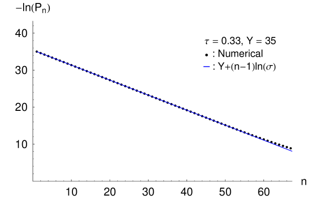
Figure 1: For high $Y$ and values of $n$ such that $n\lesssim n_{\rm cr}$ the probabilities $P_{n}(Y)$ are dominated by the first term of the sum in Eq. (3.9). Notice that for the values of $Y$ and $\tau$ used in this plot, $n_{\rm cr}\sim 67$.

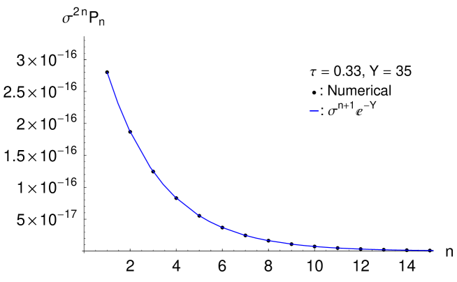
Figure 2: The distribution $\sigma^{2n}P_{n}$ as a function of $n$ for large $Y$; only the rare configurations with $n$ up to $\sim 1/\tau$ contribute to $\langle s^{2}\rangle$.

Let us verify this by explicitly computing $\langle s^{m}\rangle$, starting with $m=2$. To that aim, we separate out the contribution of the configurations with $n\lesssim n_{\rm cr}$ in Eq. (2.13) for $\langle s^{2}\rangle$. This yields

$$\langle s^{2}\rangle=\sum_{n=1}^{n_{\rm cr}}P_{n}(Y)\sigma^{2n}\simeq{\rm e}^{-Y}\sum_{n=1}^{n_{\rm cr}}\frac{\sigma^{2n}}{\sigma^{n-1}}=\frac{\sigma^{2}(1-\sigma^{n_{\rm cr}-1})}{1-\sigma}\,{\rm e}^{-Y}\,\simeq\,\frac{\sigma^{2}}{1-\sigma}\,{\rm e}^{-Y},$$ (3.17)

where the neglected terms are of $\mathcal{O}({\rm e}^{-2(Y-Y_{c})})$, and thus are exponentially suppressed when $Y\gg Y_{c}$ relatively to the dominant contribution, of $\mathcal{O}({\rm e}^{-(Y-Y_{c})})$. In practice only the configurations with up to $\sim 1/\tau$ dipoles contribute to the final result (this is manifest in Fig. 2), and for them $\sigma^{n}\mathrel{\hbox to0.0pt{\raise 2.20013pt\hbox{$>$}\hss}{\lower 2.20013pt\hbox{$\sim$}}}\sigma^{1/\tau}\sim{\rm e}^{-1}$. For any such configuration, the $S$–matrix for a projectile dipole is of order one, $s=\sigma^{n}\sim\mathcal{O}(1)$, as anticipated. The contribution of the bulk configurations with $n\mathrel{\hbox to0.0pt{\raise 2.20013pt\hbox{$>$}\hss}{\lower 2.20013pt\hbox{$\sim$}}}n_{\rm cr}$ to $\langle s^{2}\rangle$ will be considered in Sect. 3.2 and found to be of $\mathcal{O}({\rm e}^{-2(Y-Y_{c})})$, so like the terms neglected in evaluating Eq. (3.17). Hence, the final result in Eq. (3.17) gives indeed the dominant behaviour when $Y\gg Y_{c}$.

One can extend this calculation to an arbitrary $m\geq 2$. In fact, the larger $m$ is, the faster the convergence of the sum over $n$ in Eq. (2.13) is. Then it is straightforward to show that

$$\langle s^{m}\rangle\simeq\frac{\sigma^{m}}{1-\sigma^{m-1}}\,{\rm e}^{-Y}\qquad\mbox{for}\qquad m\geq 2\,.$$ (3.18)

We emphasize here that not only the $Y$–dependence, but also the prefactor in the above equation are well under control. This result is in agreement with the respective one in Eq. (3.1) and it fixes the parameter $A$ there to be $A=\sigma^{2}$.

More generally, the above procedure allows one to calculate the generating functional $Z(u,Y)$, Eq. (2.9), for large $Y$ and any value of $u$ which is strictly smaller than $\sigma$: the corresponding result is obtained by simply replacing $\sigma^{m}\to u$ in Eq. (3.18), and reads

$$Z(u,Y)\simeq\frac{u}{1-(u/\sigma)}\,{\rm e}^{-Y}\qquad\mbox{for}\quad Y\gg Y_{c}\quad\mbox{and}\quad 0\leq u<\sigma\,.$$ (3.19)

The analytic estimate (3.18) for $\langle s^{m}\rangle$ and the corresponding one for $Z(m)\equiv Z(u=\sigma^{m})$ are compared to the respective numerical results in Figs. 3 and 4.

Figure 3: The $S$–matrix for the scattering of $m$ projectile dipoles normalized to that for the scattering of two dipoles; for $Y\gg Y_{c}\approx 1.5$ and $m\geq 2$, the $Y$–dependence is the same and equal to ${\rm e}^{-Y}$.

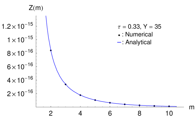
Figure 4: The generating functional as a function of $m=\ln u/\ln\sigma$ for $m>1$. When $m$ is an integer, $Z(m)$ gives the $S$-matrix for the scattering of $m$ projectile dipoles off the target.

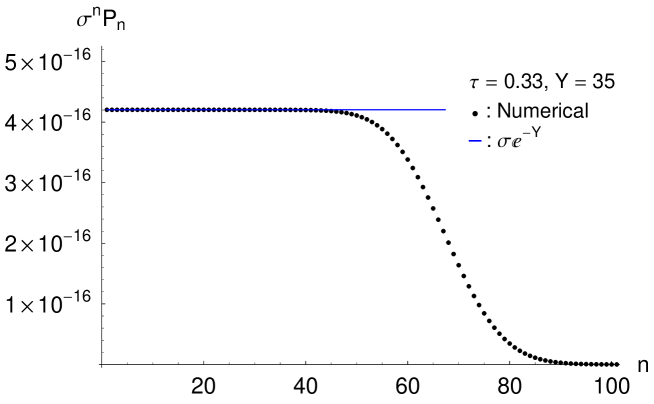
Figure 5: The distribution $\sigma^{n}P_{n}$ as a function of $n$ for large $Y$; all the configurations with $n$ up to $n_{\rm cr}\approx\sigma(Y\!-\!Y_{c})/\tau$ contribute to $\langle s\rangle$.

Let us now turn to the case $m=1$, which is special. Then the analog of Eq. (3.17) reads

$$\langle s\rangle=\sum_{n=1}^{n_{\rm cr}}P_{n}(Y)\sigma^{n}\simeq\sigma{\rm e}^{-Y}\sum_{n=1}^{n_{\rm cr}}1\,\simeq\,\frac{\sigma^{2}}{1-\sigma}\,(Y-Y_{c})\,{\rm e}^{-Y}\,,$$ (3.20)

where we have used the improved estimate $n_{\rm cr}\approx(\sigma/\tau)(Y-Y_{c})$, to be found in Sect. 3.2. The prefactor in front of the exponential in the final result is essentially the number of configurations which contribute to the average $S$–matrix, with each such configuration bringing a contribution of $\mathcal{O}({\rm e}^{-Y})$. Note, however, that the above sum is dominated by its upper limit, i.e., by configurations with $n\sim n_{\rm cr}$, for which our approximations are not fully under control. This result turns out to be nevertheless correct (up to corrections of $\mathcal{O}(1)$ to the rapidity shift $Y_{c}$, which go beyond the present accuracy), for the following reason: the distribution $\sigma^{n}P_{n}(Y)$ is almost flat as a function of $n$ so long as $n\lesssim n_{\rm cr}$ — as manifest on Eq. (3.20) — but it drops out very fast when $n>n_{\rm cr}$ (this can be seen in the numerical results in Fig. 5 and will be analytically verified in the next section).

Figure 6: The expectation value $\langle s\rangle$ of the $S$–matrix for onium–onium scattering. Starting from $\langle s\rangle_{0}=\sigma$, this expectation values falls exponentially to zero when $Y\gg Y_{c}$, in agreement with the analytic prediction (3.20) (see also Fig. (7)).

Figure 7: The average value $\langle s\rangle$ for higher values of $Y$. The analytic curve is obtained by using Eq. (3.20) with $Y_{c}=\ln(1/\tau)$.

A different way to check Eq. (3.20) is to rely on the hierarchy of evolution equations for $\langle s^{m}\rangle$. As previously noticed, $\langle s^{m}\rangle$ given by Eq. (3.18) is an accurate asymptotic solution for all the equations in the hierarchy starting with the second one. Then one can use this result, together with the first equation in the hierarchy, Eq. (2.15), in order to determine the asymptotic form of $\langle s\rangle$. Thus one easily recovers Eq. (3.20) where however the rapidity shift $Y_{c}$ is left undetermined. A further confirmation of Eq. (3.20) can be found in the original calculation of $\langle s\rangle$ by Mueller and Salam [1], which is based on the solution to Eq. (2.17) and which yields the same result as our Eq. (3.20) with $Y_{c}=\ln(1/\tau)+\mathcal{O}(1)$. The analytic estimate (3.20) is compared to the respective, exact, numerical result in Figs. (6) and (7), which confirm that both the $Y$–dependence and the normalization shown in Eq. (3.20) are indeed under control.

To conclude this section, it is instructive to compare the above results to those predicted by the dipole picture. Since the latter is not boost invariant, we shall obtain different results for $\langle s^{m}\rangle$ depending upon the system that we decide to evolve: the target or the projectile:

(i) Projectile evolution in the dipole picture. The dipole $S$–matrix elements $\langle s^{m}\rangle$ obey the Balitsky equations, that is, Eq. (2.14) with the prefactor $f_{m}$ replaced by $m$. By doing this replacement, one looses Lorentz invariance. This is formally recovered by allowing the projectile and the target to obey different evolution equations. Namely, if the projectile obeys dipole evolution, then in order for the r.h.s. of Eq. (2.12) to be independent of $Y_{0}$, the target probabilities $P_{n}^{{\rm R}}(Y-Y_{0})$ which enter $\left\langle s^{m}\right\rangle_{Y-Y_{0}}$ via Eq. (2.13) must evolve according to the ‘JIMWLK’ version of the master equation, i.e., Eq. (2.17).

Let us then estimate the high–energy behaviour of $\langle s^{m}\rangle$ as predicted by the Balitsky equations: by inserting the Ansatz $\langle s^{m}\rangle=\exp{(-c_{m}Y)}$ in this hierarchy, one immediately finds $c_{m}=m$, and hence

$$\langle s^{m}\rangle={\rm e}^{-mY}\qquad\mbox{ at large $Y$\ \ \ \ \ \ (no saturation in the projectile) }\,,$$ (3.21)

which is essentially the mean field estimate (3.2). Thus, by neglecting saturation effects in the projectile wavefunction (or, equivalently, particle–number fluctuations in the target wavefunction), we are led to the wrong conclusion that $\left\langle s^{m+1}\right\rangle$ vanishes faster than $\langle s^{m}\rangle$ at large $Y$.

(ii) Target evolution in the dipole picture. By using the target–average expression (2.13) for $\langle s^{m}\rangle$ together with the explicit solution (3.7) for the probabilities in the dipole picture, one immediately finds:

$$\langle s^{m}\rangle\simeq\frac{\sigma^{m}}{1-\sigma^{m}}\,{\rm e}^{-Y}\qquad\mbox{for $m\geq 1$ \ and \ large $Y$}\qquad\mbox{(no saturation in the target)},$$ (3.22)

where the neglected terms are of order $\mathcal{O}({\rm e}^{-2Y})$. For $m\geq 2$, this is essentially the same as the correct result at large $Y$, as given in Eq. (3.18). This agreement is consistent with the fact that $\langle s^{m}\rangle$ with $m\geq 2$ is dominated by rare target configurations with a small dipole number and thus are insensitive to saturation effects. For $m=1$, on the other hand, the dipole–picture prediction in Eq. (3.22) is different from the correct respective result in Eq. (3.20); namely, it misses the large, overall, factor $Y-Y_{c}$, which in Eq. (3.20) has been produced by summing over configurations with a relatively large number of dipoles $n\mathrel{\hbox to0.0pt{\raise 2.20013pt\hbox{$<$}\hss}{\lower 2.20013pt\hbox{$\sim$}}}(Y-Y_{c})/\tau$ (cf. Eq. (3.20)), which are close to saturation.

3.2 The bulk of the dipole distribution

Although they appeared to be quasi–irrelevant in our previous calculation of the average $S$–matrix, the typical configurations become important when this calculation is performed in a different frame. Therefore, in this subsection we study these typical configurations, i.e. the probability distribution $P_{n}(Y)$ at high energy (typically, $Y\gtrsim Y_{c}$) and for a large number of dipoles $n\gg n_{\rm sat}$.

To compute this distribution, we return to the exact Laplace transform, Eq. (3.5), and write

$$\ln[f_{n}\widetilde{P}_{n}(\omega)]=-\sum_{k=1}^{n}\ln\left(1+\frac{\omega}{f_{k}}\right)=\sum_{r=1}^{\infty}\frac{(-1)^{r}\omega^{r}}{r}\sum_{k=1}^{n}f_{k}^{-r},$$ (3.23)

where we have expanded the logarithm and exchanged the order of the two summations. We shall now perform the summation over $k$ in the above equation, under the assumptions that $n\tau\gg 1$ and $\tau\ll 1$. More precisely, we shall neglect terms which are of order (or smaller than) $\mathcal{O}{({\rm e}^{-\tau n})}$ and/or $\mathcal{O}{(\tau)}$. Notice that all these summations grow linearly with $n$ for large $n$ (since $f_{k}^{-r}\simeq\tau^{r}$ when $k\gg 1/\tau$), so it will be convenient to subtract this large contribution and then perform approximations on the remainder. We thus have

$$\Sigma_{1}\equiv\sum_{k=1}^{n}f_{k}^{-1}=\tau\sum_{k=1}^{n}\frac{1}{1-\sigma^{k}}\simeq\tau n+\tau\sum_{k=1}^{\infty}\frac{\sigma^{k}}{1-\sigma^{k}}\simeq\tau n+\ln(1/\tau)+\gamma_{\rm E},$$ (3.24)

where the third, approximate, equality has been obtained by extending the upper limit of the sum from $n$ to $\infty$, which is correct up to terms of order $\mathcal{O}{({\rm e}^{-\tau n})}$. The ensuing sum is evaluated in Appendix B under the assumption that $\tau\ll 1$. Also, $\gamma_{\rm E}=0.577...$ is the Euler constant.

Similarly for $r\geq 2$ we have (cf. Appendix B)

$$\Sigma_{r}\equiv\sum_{k=1}^{n}f_{k}^{-r}=\tau^{r}\sum_{k=1}^{n}\frac{1}{(1-\sigma^{k})^{r}}\simeq\tau^{r}n+\tau^{r}\sum_{k=1}^{\infty}\frac{1-(1-\sigma^{k})^{r}}{(1-\sigma^{k})^{r}}\simeq\tau^{r}n+\zeta(r),$$ (3.25)

where $\zeta(r)$ is the Riemann Zeta function. Note that the above summations are dominated by large values $k=\mathcal{O}(n)$, as anticipated in the discussion preceding Eq. (3.16). Using Eqs. (3.24) and (3.25), one can do the summation over $k$ in Eq. (3.23) to obtain

$$\ln[f_{n}\widetilde{P}_{n}(\omega)]\approx-\omega\ln(1/\tau)-n\ln(1+\tau\omega)+\ln\Gamma(1+\omega).$$ (3.26)

Thus we finally arrive at

$$P_{n}(Y)\simeq\tau\int\limits_{\mathcal{C}}\frac{{\rm d}\omega}{2\pi{\rm i}}\,\frac{{\rm e}^{\omega[Y-\ln(1/\tau)]}\,\Gamma(1+\omega)}{(1+\tau\omega)^{n}}\,,$$ (3.27)

which so far is valid for large $n\gg 1/\tau$ but arbitrary $Y$. It is straightforward to check that this distribution satisfies indeed the large–$n$ version of the master equation, i.e., the equation obtained from Eq. (2.3) after replacing $f_{n}\simeq 1/\tau$, as appropriate when $n\gg 1/\tau$.

Even though Eq. (3.27) is considerably simpler than the general form, it is still difficult to proceed without any further approximations, because of the presence of the Gamma function which has single poles on the negative real axis. Since we are interested in large values of $n$ and $Y$, we can evaluate the integral in Eq. (3.27) using a saddle point approximation. As we shall see, the saddle point will occur at a small value of $\omega$, so that we can replace the Gamma function by the lowest order terms in its expansion around $\omega=0$ : $\Gamma(1+\omega)\simeq 1-\gamma_{\rm E}\omega$. (This means that only the sum $\Sigma_{1}$ in Eq. (3.24) and the $\tau^{r}n$ terms of the sums in Eq. (3.25) are kept in the subsequent analysis.) We then obtain

$$P_{n}(Y)\simeq\tau\int\limits_{\mathcal{C}}\frac{{\rm d}\omega}{2\pi{\rm i}}\,\frac{{\rm e}^{\tau\omega\nu}}{(1+\tau\omega)^{n}}\simeq\frac{\tau}{\sqrt{2\pi|F^{\prime\prime}(\omega_{0})|}}\exp[F(\omega_{0})],$$ (3.28)

where we have defined the variable

$$\nu=\frac{Y-\ln(1/\tau)-\gamma_{\rm E}}{\tau}\,,$$ (3.29)

and the function

$$F(\omega)=\tau\omega\nu-n\ln(1+\tau\omega),$$ (3.30)

while the contour integral over $\omega$ has been evaluated in the saddle point approximation. For the latter to be justified, at least one of the conditions $\nu\tau\gg 1$ (i.e., $Y\gg Y_{c}\equiv\ln(1/\tau)$) and $n\tau\gg 1$ needs to be satisfied. Besides, the saddle point must obey $|\omega_{0}|\ll 1$, for consistency with the previous manipulations. Clearly, the saddle point occurs at

$$\omega_{0}=\frac{n-\nu}{\tau\nu}\,,$$ (3.31)

so the condition $|\omega_{0}|\ll 1$ is tantamount to $|n-\nu|\ll\tau\nu$. Evaluating $F$ and $F^{\prime\prime}$ at the saddle point and substituting in Eq. (3.28) we finally obtain a Poisson distribution, as anticipated:

$$P_{n}(\nu)=\frac{1}{\Gamma(n)}\,\nu^{n-1}{\rm e}^{-\nu}.$$ (3.32)

As aforementioned, this approximation is valid so long as $|n-\nu|\ll\tau\nu$. This range covers indeed the “bulk” of the distribution at large $Y$ (see also Fig. 8) : when summed over $n$ within this range, Eq. (3.32) yields a total probability equal to 1 up to terms of order $\mathcal{O}{({\rm e}^{-\tau\nu})}$. Moreover, the lower limit $n_{\rm min}=\nu-\tau\nu\equiv\sigma\nu$ is essentially the same as the upper limit (previously denoted as $n_{\rm cr}$) of the validity range of the approximation for $P_{n}$ constructed in Sect. 3.1 (which, we recall, consists in preserving only the first term in the sum in Eq. (3.9)). Indeed, if one redefines $n_{\rm cr}$ via the condition that these two approximations match with each other (up to prefactors) when $n=n_{\rm cr}$, then one finds $n_{\rm cr}=(1-\tau+\mathcal{O}{(\tau^{2})})\nu\approx n_{\rm min}$. Thus, the two approximations for $P_{n}$ at large $Y$ that we have constructed in this paper are complementary to each other, in the sense that, together, they cover all the interesting values of $n$ and they approximately match with each other at the borderline $n_{\rm min}\equiv n_{\rm cr}$ between their respective domains of validity in $n$.

Figure 8: For high $Y$ the probabilities $P_{n}(Y)$ follow a Poisson distribution for large values of $n$.

Now let us discuss some aspects of this distribution. The maximum of the distribution occurs at $n^{*}=\nu+1/2$ and the value at the maximum is $P_{n^{*}}\equiv P_{\rm max}=1/\sqrt{2\pi\nu}$, while the width of the distribution is proportional to $\sqrt{\nu}$. We need to say here that terms of order $\mathcal{O}{(\ln(1/\tau))}$ in the location of the maximum have not been kept, since this would requires a calculation of $\Sigma_{1}$ in Eq. (3.24) to $\mathcal{O}{(\tau)}$ accuracy (see Appendix B).

Figure 9: Factorization of expectation values holds only for quantities dominated by the bulk of the probability distribution; here the ratio of the (normal ordered) dipole-pair number with respect to the dipole number squared which approaches unity for $Y\gg Y_{c}$, in agreement with Eq. (3.33).

From Eq. (3.32) is is straightforward to deduce the average dipole number at high energy — one thus finds $\langle n\rangle=\nu$, which is indeed the same as in Eq. (2.23) — and, more generally, all the $k$–body dipole densities, which are readily obtained as

$$\langle n^{(k)}\rangle=\langle n\rangle^{k}=\nu^{k}\qquad\mbox{when}\qquad Y\gg Y_{c}\,.$$ (3.33)

This equation exhibits mean-field–like factorization, as expected for the bulk distribution at high density. This is illustrated in Fig. 9.

Let us now use the Poisson distribution (3.32) to compute the contribution of the bulk configurations to the expectation value of the $S$–matrix for the scattering of $m$ external dipoles. One thus finds

$$\langle s^{m}\rangle_{\rm bulk}=\,\sigma^{m}\,{\rm e}^{-f_{m}\tau\nu}\sim\,\langle s\rangle_{\rm bulk}^{f_{m}},$$ (3.34)

as expected from the mean field approximation, cf. Eq. (3.2). However, for $m\geq 2$, this bulk contribution is exponentially smaller (at large $\tau\nu\simeq Y-Y_{c}$) than the respective contribution of the rare configurations with only few dipoles, as previously computed in Eq. (3.18). Also, even for $m=1$, the result above is smaller by a large factor $1/(\tau\nu)\ll 1$ than the previous result in Eq. (3.20), which, we remember, is due to the configurations with $n\mathrel{\hbox to0.0pt{\raise 2.20013pt\hbox{$<$}\hss}{\lower 2.20013pt\hbox{$\sim$}}}n_{\rm cr}$. Thus, the present calculation of the bulk distribution confirms our previous conclusion that the $S$–matrix is dominated by the rare configurations which involve relatively few dipoles.

The above results enable us to also compute the high–energy behaviour of $Z(u,Y)$ for $u$ within the range $\sigma<u<1$, and thus complete our previous estimate, Eq. (3.19). Indeed, for large $Y$ and $u>\sigma$, $Z(u,Y)$ is dominated by the typical configurations, distributed according to Eq. (3.32). By using the latter within Eq. (2.9), one easily finds

$$Z(u,Y)\approx\exp\left\{-\frac{1-u}{\tau}(Y-Y_{c})\right\}\qquad\mbox{for}\quad Y\gg Y_{c}\quad\mbox{and}\quad\sigma<u<1.$$ (3.35)

The support of this function is strongly peaked near $u=1$, within a distance $1-u\sim\tau/(Y-Y_{c})$ which becomes smaller and smaller with increasing energy and/or decreasing $\tau$. But if we let $Y\to\infty$ for fixed $u<1$ (even arbitrarily close to 1), then $Z(u,Y)$ vanishes exponentially, which is another manifestation of the ‘black disk’ limit in our model.

3.3 More on boost invariance and the initial conditions

Although the average $S$–matrix is frame–independent, by construction, within the model under consideration, the physical picture of the collision — in the sense of relevant configurations — depends very much upon the choice of the frame, as we shall now demonstrate via some explicit calculations. (This dependence has been previously noticed in Refs. [1, 12].) To that aim, it is convenient to consider the (toy–model analog of) dipole–nucleus scattering; that is, we shall assume that, at $Y=0$, the target is made with $A\geq 2$ dipoles, whereas the projectile contains only one dipole: $P_{n}^{\rm R}(0)=\delta_{nA}$ and $P_{m}^{\rm L}(0)=\delta_{m1}$. Note that this is the same physical problem as considered in Sect. 3.1 — one onium starts as a single dipole in its rest frame, while the other one starts as a collection of exactly $A$ dipoles (with $A$ denoted as $m$ in Sect. 3.1) — but the terminology that we use is now different (in the sense of interchanging what we call ‘target’ and ‘projectile’), since we feel that the present terminology is more natural in relation with a physical dipole–nucleus scattering.

For the aforementioned initial conditions, we shall compute the average $S$–matrix in two different frames: the rest frame of the target (nucleus) and, respectively, that of the projectile (dipole). For more clarity, we shall denote the results of these two calculations by $\left\langle S\right\rangle_{1\times A}$ and, respectively, $\left\langle S\right\rangle_{A\times 1}$. More general initial conditions will be briefly discussed towards the end.

(a) Target (nucleus) rest frame. When the nucleus is at rest, the whole evolution is given to the dipole wavefunction. This is precisely the situation analyzed in Sect. 3.1, from which we simply quote here the final result (cf. Eq. (3.18) with $m\to A$) :

$$\left\langle S\right\rangle_{1\times A}=\frac{\sigma^{A}}{1-\sigma^{A-1}}\,{\rm e}^{-Y}\qquad\mbox{for}\qquad A\geq 2\qquad(\text{nucleus rest frame})\,.$$ (3.36)

As also discussed in Sect. 3.1, in this frame the average $S$–matrix is dominated by rare configurations in the evolved system (the ‘dipole’).

(b) Projectile (dipole) rest frame. This situation is new with respect to Sect. 3.1, in the sense that the whole evolution is now given to a system which starts with more than one dipole at $Y=0$ (the ‘nucleus’). For simplicity we shall consider first the case $A=2$ and then return to generic values for $A$. From the arguments in Sect. 3.1, one may expect the average $S$–matrix to be controlled by the rare configurations in the evolved nucleus which are dilute (but this expectation turns out to be wrong !), so let us first compute the respective contribution to $\left\langle S\right\rangle$. Following the steps given in Sect. 3.1, but now with a different initial condition, it is straightforward to find that the distribution of the rare configurations reads

$$P_{n}^{A=2}(Y)\simeq\frac{f_{n-1}}{\sigma^{2n-4}}\,{\rm e}^{-f_{2}Y}\qquad\text{for}\qquad 2\leq n\lesssim n_{\rm cr}\,,$$ (3.37)

where $n_{\rm cr}$ is basically the same as before, i.e., $n_{\rm cr}\approx(\sigma/\tau)(Y-Y_{c})$. (Note, however, that the value of $Y_{c}$ depends upon $A$; see the discussion around Eq. (3.40) below.) At a first glance, this result seems to imply that the average $S$–matrix will be proportional to ${\rm e}^{-f_{2}Y}$, which would be at variance with the previous result, Eq. (3.36), obtained in the nucleus rest frame and thus would signal a violation of the boost invariance. However, this is not really the case, since the summation over the dilute configurations is not convergent anymore, rather it is dominated by its upper limit $n_{\rm cr}$ (which, we recall, is the borderline towards the bulk configurations). Specifically,

$$\left\langle S\right\rangle_{A\times 1}\sim\sum_{n=2}^{n_{\rm cr}}\sigma^{n}P_{n}^{A=2}(Y)\sim{\rm e}^{-f_{2}Y}\sum_{n=2}^{n_{\rm cr}}\sigma^{-n}\sim\,{\rm e}^{-Y}\,,$$ (3.38)

where only the dominant exponential behaviour has been kept, and this comes from the terms with $n\simeq n_{\rm cr}$, as anticipated. This should be contrasted with the calculation in the nucleus rest frame where the corresponding sum, cf. Eq. (3.17), is rapidly convergent.

The above argument also shows that, in the present frame, $\left\langle S\right\rangle$ is rather dominated by the typical configurations in the evolved nucleus. Returning to the case of arbitrary $A\geq 2$, and following the procedure of Sect. 3.2 with the modified initial condition $P_{n}(0)=\delta_{nA}$, one finds that the precise form of the Poisson distribution which describes the bulk is

$$P_{n}^{A}(Y)=\frac{1}{(n-A)!}\,\nu^{n-A}\,{\rm e}^{-\nu}\,,$$ (3.39)

with $\nu=[Y-Y_{c}(A)]/\tau$, and where the critical rapidity $Y_{c}(A)$, determining the transition of the nucleus from the unsaturated “phase” to the saturated one, reads (for $\tau\ll 1$)

$$Y_{c}(A)=\begin{cases}\displaystyle{\ln\frac{1}{A\tau}}&\text{ for\,\, $A\tau\ll 1$}\\ \displaystyle{0}&\text{ for\,\, $A\tau\gg 1$}\,.\end{cases}$$ (3.40)

(Indeed, when $A\tau\gg 1$, the nucleus is saturated already at $Y=0$. On the other hand, when $A\tau\ll 1$, the nucleus is dilute in the early stages of the evolution, when the average dipole number rises like $\langle n\rangle=A{\rm e}^{Y}$, cf. Eq. (2.23), until it reaches a saturation value of $\mathcal{O}{(1/\tau)}$; this happens when $Y\sim Y_{c}$ with $Y_{c}$ as given above.) Given the probability distribution Eq. (3.39), it is straightforward to calculate the average $S$–matrix for the scattering of one dipole off the bulk distribution of the nucleus. One finds

$$\left\langle S\right\rangle_{A\times 1}\,\approx\,\sigma^{A}\,{\rm e}^{-[Y-Y_{c}(A)]}\,\approx\,\begin{cases}\displaystyle{\frac{\sigma^{A}}{A\tau}\,{\rm e}^{-Y}}&\text{ for\,\, $A\tau\ll 1$}\\[8.5359pt] \displaystyle{\sigma^{A}\,{\rm e}^{-Y}}&\text{ for\,\, $A\tau\gg 1$}\end{cases}\qquad(\text{dipole rest frame})\,.$$ (3.41)

Thus is the final result in the dipole rest frame and is indeed in agreement with the corresponding one in the nucleus rest frame, as given in Eq. (3.36), so long as $\tau\ll 1$ and $A\gg 1$.

Thus we see that, whether the (average) $S$–matrix is dominated by rare configurations or the bulk distribution, really depends upon the frame that one decides to view the process in. This is not perhaps not so surprising, since it reflects the fact that the wavefunction of an evolved hadron is not a frame independent quantity.

Notice also that there is some loss of accuracy when working with the bulk distribution rather than with the rare configurations: although the results (3.36) and (3.41) are consistent with each other within their validity ranges, the former is exact at high energy (i.e., it holds for any values of $\tau$ and $A$), whereas the latter is only approximate (in our second calculation, based on the bulk distribution, we have not been able to obtain the expression of the prefactor when $A\tau\sim 1$).

Now let us consider that the two systems are initially composed of $A$ and $B$ dipoles respectively, i.e. $P_{n}^{{\rm R}}(0)=\delta_{nA}$ and $P_{m}^{{\rm L}}(0)=\delta_{mB}$, and let us momentarily assume that $A<B$. From the previous discussion one understands that it is advantageous to work in the rest frame of the left mover. Then one can compute the asymptotic form of the average $S$-matrix, since it is dominated by the rare configurations of the right mover wavefunction, and one finds

$$\left\langle S\right\rangle_{A\times B}\simeq\begin{cases}\displaystyle{\frac{\sigma^{AB}}{\prod_{k=1}^{A}(1-\sigma^{B-k})}\,{\rm e}^{-f_{A}Y}}&\text{ for \,\, $A<B$}\\[14.22636pt] \displaystyle{\frac{\sigma^{A(A+1)}}{\prod_{k=1}^{A}(1-\sigma^{A+1-k})}\,Y{\rm e}^{-f_{A}Y}}&\text{ for\,\, $A=B$}\,.\end{cases}$$ (3.42)

The average $S$-matrix for the special case $A=B$, has been obtained from the $A$-th equation of the hierarchy in Eq. (2.14), after $\left\langle S\right\rangle_{A\times(A+1)}$ has been determined. Notice that Eq. (3.42) is an exact solution to this hierarchy.

More generally, one could imagine that the initial wavefunctions are determined by some smooth distributions in the number of dipoles (rather than by a given number of dipoles). Then one can determine the $S$-matrix, by averaging $\left\langle S\right\rangle_{A\times B}$ over the initial conditions. So long as $P_{1}^{\rm R}(0)$ and $P_{1}^{\rm L}(0)$ are non–zero, the asymptotic behaviour is simply given by the appropriate generalization of Eq. (3.20), namely

$$\left\langle S\right\rangle=\sum_{A,B=1}^{\infty}P_{A}^{{\rm R}}(0)P_{B}^{{\rm L}}(0)\left\langle S\right\rangle_{A\times B}\simeq P_{1}^{\rm R}(0)P_{1}^{\rm L}(0)\,\frac{\sigma^{2}}{1-\sigma}\,Y{\rm e}^{-Y}\,,$$ (3.43)

since the term $A=B=1$ dominates the double sum when $Y\to\infty$.

4 Correspondence between the toy model and high energy QCD

Throughout this paper, we have emphasized similarities between the structure and the predictions of the toy model and the known or expected properties of high–energy QCD. In what follows, we discuss this correspondence in a more systematic way.

The factorization formula for the $S$–matrix, Eq. (2.1), is reminiscent of the factorization schemes proposed within high–energy QCD in Refs. [3, 48, 11, 22, 23], which have in common to be symmetric between the projectile and the target. With the noticeable exception of the dipole factorization [3], which however fails to accommodate the saturation effects in the wavefunctions of the colliding hadrons, all the other schemes alluded to above are not written in terms of particle numbers, but rather in terms of gluon fields, sometimes represented (in the CGC formalism [37]) as classical color charges together with the color fields they radiate. It is therefore essential to establish the proper correspondence between gluons in QCD and particles in the toy model.

This correspondence goes as follows: the ‘dipoles’ in the toy model correspond to $s$–channel gluons in QCD (so like the real color dipoles in Mueller’s dipole picture), while $\tau=1-\sigma$ corresponds to gluons exchanged in the $t$–channel. (The analog of $\tau$ in QCD starts at order $\alpha_{s}^{2}$, corresponding to a two–gluon exchange between a pair of dipoles.) Hence, in an effective gluon language, the evolution described by Eqs. (2.3) and (2.5) contains vertices for gluon splitting in the $s$–channel — these are, of course, the vertices $f_{n}$ — and also vertices for both splitting and merging in the $t$–channel — each exchange $\tau$ being sandwiched between two such vertices. Hence, this evolution constructs the analog of the ‘Pomeron loops’ in the onium wavefunction. Fully symmetric ‘Pomeron loops’ will develop, of course, in the $S$–matrix for onium–onium scattering, as described by Eq. (2.1).

With this identification, the toy–model hierarchy for the dipole scattering amplitudes, cf. Eqs. (2.14) or (2.19)–(2.21), corresponds to the QCD evolution equations with Pomeron loops, as constructed in Refs. [17, 18, 19]. To render this analogy more precise, let us focus first on the case where Pomeron loops are absent, and for which the toy model version is given in Eqs. (2.17) and (2.18). We would like to argue that the continuum version of the master equation, Eq. (2.17), is the toy–model analog of the JIMWLK equation in QCD. The JIMWLK equation [7, 8, 9] is written for the color fields $A^{+}_{a}\equiv\alpha^{a}$ radiated in the $t$–channel by the gluons produced in the $s$–channel by the high–energy evolution of the (right–moving) target. It is a second–order, functional, differential equation with respect to $\alpha$ and reads, schematically,

$$\frac{\partial W_{Y}[\alpha]}{\partial Y}\,=\,\frac{1}{2}\frac{\delta}{\delta\alpha_{a}}\,\chi^{ab}[\alpha]\frac{\delta}{\delta\alpha_{b}}\,W_{Y}[\alpha]\,,$$ (4.1)

where the transverse coordinates have not been shown. The quantity $W_{Y}[\alpha]$ is the probability distribution for the fields $\alpha_{a}$ (the analog of $P_{n}(Y)$ of the toy model). The kernel $\chi^{ab}[\alpha]$ — the analog of the emission rate $f_{n}$ — is non–linear in $\alpha$ to all orders, via Wilson lines. These describe the multiple scattering of the gluon emitted in the $s$–channel in the last step of the evolution off the background field $\alpha$ (the $t$–channel gluons) produced by the previous steps of the evolution; this rescattering is similar to that included in $f_{n}$ within the toy model. To complete the identification between Eqs. (4.1) and (2.17), one should recall that in the JIMWLK equation each $s$–channel gluon is allowed to radiate only two gluons in the $t$–channel. Hence, the second–order derivative w.r.t. $\alpha$ in Eq. (4.1) can be interpreted as a single derivative w.r.t. $n$ (the number of gluons in the $s$–channel) and then Eq. (4.1) becomes indeed similar to Eq. (2.17).

Strictly speaking, the JIMWLK equation does include some fluctuations, since it is Fokker–Planck equation for a random walk in the functional space of color fields[10]. However, these are merely color fluctuations which are suppressed at large $N_{c}$. The essential correlations associated with gluon–number fluctuations are lost because of the impossibility to probe both ($s$–channel) gluons which are produced after one splitting. This is related to the fact that, as aforementioned, an $s$–channel gluon cannot radiate more than two $t$–channel fields, and thus cannot undergo multiple scattering off the projectile. By contrast, within the toy model, the dipoles are allowed to scatter multiply — both inside the target wavefunction and with the dipoles in the projectile —, hence the $n$–body correlations associated with splitting are fully taken into account. In the language of QCD, each $s$–channel gluon is allowed to absorb and radiate an arbitrary number of $t$–channel gluons, so like in the more general, ‘self–dual’, evolution described in Refs. [24, 25].

In fact, as noticed in Ref. [33], the structure of the master equation for the toy model bears some formal resemblance to that of the ‘diamond’ Hamiltonian constructed in Refs. [24, 25]. In particular, it shares with the latter the property of being self–dual, as it should, since the self–duality of the Hamiltonian is equivalent to the fact that the $S$-matrix is boost–invariant, when the latter is given by a factorization formula like the one in Eq. (2.1) [22, 23]. To see this, note that the master equation can be rewritten as (cf. Eqs. (2.3) and (2.5))

$$\frac{{\rm d}P_{n}(Y)}{{\rm d}Y}\,=\,-\,\frac{1}{\tau}\,\Big{(}1-{\rm e}^{-\frac{\partial}{\partial n}}\Big{)}\Big{(}1-{\rm e}^{-n|\ln\sigma|}\Big{)}\,P_{n}(Y)\,\equiv\,H\Big{[}n|\ln\sigma|,\frac{\partial}{\partial n}\Big{]}P_{n}(Y)\,,$$ (4.2)

where we have extended $n$ to be a continuum variable and used $g(n-1)=\exp(-{\rm d}/{\rm d}n)g(n)$ for a generic function $g(n)$. As anticipated, the ‘Hamiltonian’ appearing in Eq. (4.2) is ‘self–dual’ [33], that is, it is invariant under the self–duality transformation which in the present context consists in exchanging

$$\frac{\partial}{\partial n}\ \longleftrightarrow\ n|\ln\sigma|\,,$$ (4.3)

and then reversing the order of the operators. Moreover, the presence of two types of exponentials — one involving the number of particles $n$ and one involving the derivative ${\partial}/{\partial n}$ — is reminiscent of the two types of Wilson lines which appear in the QCD Hamiltonian proposed in Refs. [24, 25]. In QCD, $n|\ln\sigma|$ is replaced by the color field produced by the $s$–channel gluons, and ${\partial}/{\partial n}$ by the (functional) derivative with respect to the color charge density of these gluons.

Let us now return to the equations obeyed by the dipole scattering amplitudes and compare the structure of the fluctuation terms between the toy model and QCD. Consider first the equation for $\langle t^{2}\rangle$, as displayed in Eq. (2.20) for the toy model and, respectively, in Eqs. (2.7) and (2.8) of Ref. [18] for QCD. In both cases, the dominant fluctuation term is of the generic type $\tau\langle t\rangle$, i.e., it is linear in $\langle t\rangle$ and of order $\tau\sim\alpha_{s}^{2}$. Yet, the experience with the toy model tells us that the coefficient of the fluctuation term in QCD (cf. Eq. (2.7) in Ref. [18]) may actually be incomplete. Indeed, in the calculation of this term in Refs. [17, 18, 19] one has neglected the possibility that the individual dipoles from the target undergo multiple scattering with the dipoles in the projectile; that is, in deriving the equation for $\langle t^{2}\rangle$, the two external dipoles have been allowed to scatter only with two different dipoles from the target (but not also to scatter both off a same dipole). By contrast, in the toy model calculation, multiple scattering is included and is in fact responsible for an $\mathcal{O}{(1)}$ contribution to the coefficient of fluctuation term $\tau\langle t\rangle$ in Eq. (2.20) : if that contribution was neglected, the ensuing coefficient would be twice as large than the correct one. More generally, if one considers the equation satisfied by $\langle t^{m}\rangle$ within the toy model, then among the $m-1$ (relevant) fluctuation terms which are included in this equation (cf. Sect. 2.2) — namely, $\tau\langle t^{m-1}\rangle$, $\tau^{2}\langle t^{m-2}\rangle$, $\dots$, $\tau^{m-1}\langle t\rangle$ — only the analog of the first term, $\tau\langle t^{m-1}\rangle$, has been so far included in the corresponding equation in QCD [18].

This discussion allows us to draw some lessons for QCD: most likely, the Pomeron loop equations in QCD at large $N_{c}$ should be completed by including the effects of the multiple scattering of the individual target dipoles. This conclusion appears to be in conflict with some recent analyses within QCD [49, 50], which should be therefore carefully reexamined. Furthermore, the more intricate structure for the fluctuation terms suggested by the toy model seems to prevent one from mapping the problem under study into a single Langevin equation. Note that, although the detailed structure of the fluctuation terms in QCD may be indeed more complicated than anticipated by the original analysis in Refs. [17, 18, 19, 23], it is possible that the additional terms will not modify the qualitative asymptotic behaviour of the dipole scattering amplitudes at high energy and large $N_{c}$. As argued in Refs. [15, 17], this behaviour seems to be dictated simply by the stochastic nature of the evolution equations.

An other interesting result of the toy model that we expect to extend to QCD as well is the fact that the average $S$–matrix in the vicinity of the unitarity limit is dominated by rare fluctuations with only few gluons. This is in agreement with the arguments presented in that sense in Refs. [1, 12], which also show that the exponential approach towards the black disk limit should be somehow faster in QCD, namely like $\langle s\rangle\sim\exp(-Y^{2})$, to be compared with the toy–model result $\langle s\rangle\sim\exp(-Y)$. (The additional factor of $Y$ in QCD comes from the phase–space for diffusion in the dipole transverse sizes.) But what is most interesting about our present results is that the $S$–matrix $\langle s^{m}\rangle$ for the simultaneous scattering of several dipoles is even more strongly dominated by the rare fluctuations which are dilute, to the point that $\langle s^{m}\rangle$ with $m\geq 2$ is not at all sensitive to saturation effects in the target wavefunction, and (unlike $\langle s\rangle$) it could have been simply computed within the dipole picture. It would be interesting to understand whether a similar feature holds in QCD as well. If so, this would mean that, for $m\geq 2$, $\langle s^{m}\rangle$ in high–energy QCD at large $N_{c}$ can be reliably computed via numerical simulations within Mueller’s dipole picture.

Appendix A Lack of boost invariance for the recombination process

In this appendix, we shall consider more general (zero–dimensional) models in which in addition to particle splitting, one allows for recombination. The simplest model of this type is the reaction model $A\rightleftharpoons AA$, introduced in the context of QCD in Ref. [17], and further discussed in Refs. [32, 34, 35]. In that model, a particle can split into two ($A\to AA$) at a rate $\alpha$ per particle and, conversely, two particles can recombine into one ($AA\to A$) with a rate $\beta$ per pair of particles. In what follows, we shall consider a more general version of this model, in which the rates for splitting ($f_{n}$) and merging ($g_{n}$) are taken to be general functions of the number $n$ of particles in the system. Hence, in such a process, particle number saturation can in principle occur via two different mechanisms: the saturation of the rate for particle splitting and the particle recombination.

However, as we shall show in what follows, the recombination process cannot be made consistent with the boost invariance of the $S$–matrix (within the factorization scheme of Eq. (2.1)) for any choice of the $g_{n}$’s. This finding, together with the fact that, within the context of the JIMWLK equation, gluon saturation occurs via the saturation of the emission rate, suggests that the models based on recombination may not closely resemble the QCD dynamics. This conclusion is further supported by the observation in Ref. [26] that, if one attempts to interpret the Pomeron loop equations of QCD [17] as a reaction–diffusion process (in either the target or the projectile), then one is lead to introduce an effective ‘recombination vertex’ which has no definite sign, and hence no probabilistic interpretation.

The master equation is obtained by adding to the r. h. s. of Eq. (2.3) the terms responsible for recombination. We thus obtain

$$\frac{{\rm d}P_{n}(Y)}{{\rm d}Y}=f_{n-1}\,P_{n-1}(Y)-f_{n}\,P_{n}(Y)+g_{n+1}\,P_{n+1}(Y)-g_{n}\,P_{n}(Y),$$ (A.1)

where the functions $f_{n}$ and $g_{n}$ should be chosen so as to ensure the boost invariance of the $S$–matrix and satisfy the boundary conditions $f_{1}=\alpha$ and $g_{1}=0$. By requiring the average $S$–matrix in Eq. (2.1) to be independent of $Y_{0}$, we easily obtain the following constraint

$$f_{m}(1-\sigma^{n})-f_{n}(1-\sigma^{m})-g_{m}(\sigma^{-n}-1)+g_{n}(\sigma^{-m}-1)=0.$$ (A.2)

A priori, there are two different ways in which this constraint could be satisfied: (i) the independent cancellation of the $f$-terms and $g$-terms, and (ii) the mutual cancellation between the two types of terms. Both are excluded, as we now show.

(i) By requiring the independent cancellation of the $f$-terms and the $g$-terms in Eq. (A.2), one finds

$$f_{n}=c\,(1-\sigma^{n})\quad\text{and}\quad g_{n}=d\,(\sigma^{-n}-1),$$ (A.3)

where the constants $c$ and $d$ are determined by the boundary conditions at $n=1$. For $f_{n}$ we recover Eq. (2.5), but the condition $g_{1}=0$ can be satisfied only by choosing $d=0$, and hence $g_{n}=0$ for any $n$.

(ii) In order for the $f$-terms to cancel against the $g$-terms in Eq. (A.2) one needs

$$f_{n}=c\,(\sigma^{-n}-1)\quad\text{and}\quad g_{n}=-c\,(1-\sigma^{n}).$$ (A.4)

Depending on the sign of the constant $c$, either the $f_{n}$’s or the $g_{n}$’s will be negative, and thus there is no probabilistic interpretation — a situation reminiscent of the difficulty met in Ref. [26].

The standard reaction–diffusion process $A\rightleftharpoons AA$ is defined by (see, e.g., [17])

$$f_{n}=\alpha n\quad\text{and}\quad g_{n}=\beta n(n-1)/2,$$ (A.5)

and thus it does not belong to the case (ii); this process has a well–defined probabilistic interpretation, but is inconsistent with the boost invariance of the $S$–matrix in the factorization scheme of Eq. (2.1), which includes multiple scattering for the individual particles.

To better appreciate this difficulty, let us explicitly compute, within the reaction model of Eq. (A.5), the high–energy limit of the average $S$–matrix for ‘dipole–nucleus scattering’ — i.e., for the scattering between two onia which in their respective rest frames reduce to a single dipole in the case of the projectile and, respectively, to a set of $A$ dipoles, with $A\geq 1$, in the case of the target — by separately working in the target rest frame and in the projectile rest frame. We anticipate that the final results will be non–zero in both cases (in agreement with the ‘grey disk limit’ reported in Ref. [35]), but different for the two calculations. Only one of these results will correspond to that found in Ref. [35], which has adopted the point of view of the projectile evolution.

Before we proceed, let us notice that, within the reaction model of Eq. (A.5), the quantities $\alpha$, $\beta$ and $\sigma$ are a priori independent parameters (the first two of them referring to the evolution of the onium wavefunction, and the third one characterizing the elementary dipole–dipole scattering), but in view of the correspondence with QCD one needs to assume that the ratio $\beta/\alpha$ is of the same order as $\tau\equiv 1-\sigma$, namely they are both of $\mathcal{O}{(\alpha_{s}^{2})}$ (in particular, this implies $\beta\ll\alpha$). To facilitate the comparison between this model and the one studied in this paper, we denote $\beta/2\alpha\equiv\tau_{0}$, with $\tau_{0}\sim\tau\ll 1$.

We start by summarizing the formulæ giving $\left\langle S\right\rangle_{Y}$ in the considered frames:

(a) Target (nucleus) rest frame (i.e., projectile evolution). This is the case $Y_{0}=Y$ in Eq. (2.1), which then implies:

$$\left\langle S\right\rangle_{Y}^{{\rm L}}=\sum_{m}P_{m}^{{\rm L}}(Y)\,\,\sigma^{mA}\,=\,Z^{{\rm L}}(u=\sigma^{A},Y),$$ (A.6)

where $P_{m}^{{\rm L}}(0)=\delta_{m1}$, so that $Z^{{\rm L}}(u,Y=0)=u$.

(b) Projectile (dipole) rest frame (i.e., target evolution). In this case, $Y_{0}=0$ and Eq. (2.1) implies:

$$\left\langle S\right\rangle_{Y}^{{\rm R}}=\sum_{n}P_{n}^{{\rm R}}(Y)\,\,\sigma^{n}\,=\,Z^{{\rm R}}(u=\sigma,Y),$$ (A.7)

where this time $P_{n}^{{\rm R}}(0)=\delta_{nA}$, implying $Z^{{\rm R}}(u,Y=0)=u^{A}$.

We have related here $\left\langle S\right\rangle_{Y}$ to the generating functional $Z(u,Y)$, cf. Eq. (2.13), since as shown in Ref. [35] the latter is the quantity which is most conveniently evaluated in the context of the reaction model. Specifically, it is first straightforward to use Eq. (A.1) with the vertices $f_{n}$ and $g_{n}$ from Eq. (A.5) to deduce the following evolution equation for $Z(u,Y)$ in the reaction model (to be compared to Eq. (2.11)) :

$$\frac{{\rm d}Z}{{\rm d}Y}\,=\,u(1-u)\left\{-\alpha\,\frac{\partial Z}{\partial u}\,+\,\frac{\beta}{2}\,\frac{\partial^{2}Z}{\partial u^{2}}\right\}.$$ (A.8)

This equation is the starting point of the analysis in Ref. [35]. As shown there, and it can be also easily verified by inspection, this equation admits the following, non–trivial, fixed point

$$Z_{\infty}(u)\,=\,\frac{{\rm e}^{u/\tau_{0}}-1}{{\rm e}^{1/\tau_{0}}-1}\,,\qquad(\tau_{0}\equiv\beta/2\alpha),$$ (A.9)

which, as anticipated by our notations, is the same as the high–energy limit of the physical generating functional (i.e., the solution to Eq. (A.8) with physical initial conditions) : $Z(u,Y\to\infty)\to Z_{\infty}(u)$ for any initial conditions. (This is demonstrated in Ref. [35].) This should be contrasted to the corresponding behaviour of the model studied by us here, where we have seen that $Z(u,Y)$ vanishes exponentially when $Y\to\infty$ for any $u<1$ (cf. Eqs. (3.19) and (3.35)).

By substituting Eq. (A.9) in Eqs. (A.6) and (A.7), it is easy to compute the asymptotic values of the (average) $S$–matrix in the two Lorentz frames under consideration. Explicitly, one obtains

$$\left\langle S\right\rangle_{\infty}^{{\rm L}}\,=\,\frac{{\rm e}^{\sigma^{A}/\tau_{0}}-1}{{\rm e}^{1/\tau_{0}}-1}\,\simeq\,{\rm e}^{-(1-\sigma^{A})/\tau_{0}}\,-\,{\rm e}^{-1/\tau_{0}}\,,$$ (A.10)

where the second, approximate, equality holds since $\tau_{0}\ll 1$. The quantity $1-\sigma^{A}$ can be recognized as the original value of the scattering amplitude at $Y=0$: $\left\langle T\right\rangle_{0}=1-\left\langle S\right\rangle_{0}=1-\sigma^{A}$. It is not hard to show that $\left\langle S\right\rangle_{\infty}^{{\rm L}}<\left\langle S\right\rangle_{0}=\sigma^{A}$ for any positive value of $\tau_{0}$ and any value of $\sigma^{A}$ such that $0<\sigma^{A}<1$. Thus, in this case, one reaches the natural conclusion that the value of the $S$-matrix becomes smaller at high energy.

On the other hand,

$$\left\langle S\right\rangle_{\infty}^{{\rm R}}\,=\,\frac{{\rm e}^{\sigma/\tau_{0}}-1}{{\rm e}^{1/\tau_{0}}-1}\,\simeq\,{\rm e}^{-\tau/\tau_{0}}\,-\,{\rm e}^{-1/\tau_{0}}\,,$$ (A.11)

where the exponent $\tau/{\tau_{0}}$ is of order one. Clearly, for any $A>1$, the two above results are different from each other, namely, one has $1-\sigma^{A}>1-\sigma\equiv\tau$ and hence $\left\langle S\right\rangle_{\infty}^{{\rm L}}<\left\langle S\right\rangle_{\infty}^{{\rm R}}$.

Moreover, when $A$ is large enough, the results above predict that the asymptotic $S$–matrix at high energy may become larger than the original $S$–matrix $\left\langle S\right\rangle_{0}=\sigma^{A}$ at $Y=0$. Indeed, by using $|\ln\sigma|\simeq\tau$, one can easily check that $\left\langle S\right\rangle_{\infty}^{{\rm R}}>\sigma^{A}$ as soon as $A>1/\tau_{0}$.

Appendix B A useful sum

In this Appendix we calculate the following sum (with $\sigma=1-\tau$)

$$\mathcal{S}_{1}(\tau)\equiv\tau\sum_{n=1}^{\infty}\frac{\sigma^{n}}{1-\sigma^{n}}.$$ (B.1)

Up to the $\tau$ prefactor, this is equal to the double sum $\sum_{m,n=1}^{\infty}\sigma^{mn}$, which cannot be written in terms of known functions. Nevertheless, we can obtain an analytic expression for $\tau\ll 1$, by keeping the first few terms in a series expansion. Here we shall work up to order $\mathcal{O}{(\tau)}$. (Of course, the summation can be easily evaluated numerically, since it is rapidly convergent for any $\sigma<1$.)

One can convert the sum into an integral by making use of the Euler–McLaurin summation formula, which may be written as

$$\sum_{n=1}^{\infty}h_{n}=\int\limits_{1}^{\infty}{\rm d}n\,h(n)+\frac{1}{2}\,h(1)+2\sum_{k=1}^{\infty}\frac{(-1)^{k}\zeta(2k)}{(2\pi)^{2k}}\,h^{(2k-1)}(1).$$ (B.2)

With $h(n)=\tau\sigma^{n}/(1-\sigma^{n})$, it is straightforward to calculate the integral and obtain

$$\int\limits_{1}^{\infty}{\rm d}n\,\frac{\tau\sigma^{n}}{1-\sigma^{n}}=\frac{\tau\ln\tau}{\ln(1-\tau)}=\ln\frac{1}{\tau}-\frac{1}{2}\,\tau\ln\frac{1}{\tau}+\mathcal{O}{(\tau^{2})}.$$ (B.3)

The integral contains the dominant contribution for small $\tau$, which is equal to $\ln(1/\tau)$. It is trivial to obtain the contribution of the second term in Eq. (B.2) which is

$$\frac{1}{2}\,h(1)=\frac{1}{2}-\frac{\tau}{2}.$$ (B.4)

For the contribution of the third term in Eq. (B.2) we need the $(2k\!-\!1)$-th derivative of $h(n)$ at $n=1$ which, to the order of interest, reads

$$h^{(2k-1)}(1)=-\Gamma(2k)\left(1-\frac{\tau}{2}\right)+\mathcal{O}{(\tau^{2})}.$$ (B.5)

Notice that we have to sum a series whose terms are growing factorially. However, the terms have alternating signs and the series is Borel summable. Thus we can write the third term as

$$-2\left(1-\frac{\tau}{2}\right)\sum_{k=1}^{\infty}\frac{(-1)^{k}\,\zeta(2k)\,\Gamma(2k)}{(2\pi)^{2k}}$$ (B.6)

$$= -2\left(1-\frac{\tau}{2}\right)\int\limits_{0}^{\infty}\frac{{\rm d}b}{b}\,{\rm e}^{-b}\sum_{1}^{\infty}(-1)^{k}\,\zeta(2k)\left(\frac{b}{2\pi}\right)^{2k}$$

$$= \left(1-\frac{\tau}{2}\right)\int\limits_{0}^{\infty}\frac{{\rm d}b}{b}\,{\rm e}^{-b}\,\left[\frac{b}{2}\,\coth\left(\frac{b}{2}\right)-1\right]=\left(\gamma_{\rm E}-\frac{1}{2}\right)\left(1-\frac{\tau}{2}\right).$$

Adding the three contributions obtained in Eqs. (B.3), (B.4) and (B.6) we finally arrive at

$$\mathcal{S}_{1}(\tau)=\ln\frac{1}{\tau}+\gamma_{\rm E}-\frac{1}{2}\,\tau\ln\frac{1}{\tau}-\frac{1+2\gamma_{\rm E}}{4}\,\tau+\mathcal{O}{(\tau^{2})}.$$ (B.7)

Similarly one can obtain the other sums encountered in Eq. (3.25). One finds

$$\mathcal{S}_{r}(\tau)\equiv\tau^{r}\sum_{n=1}^{\infty}\frac{1-(1-\sigma^{n})^{r}}{(1-\sigma^{n})^{r}}=\zeta(r)+\mathcal{O}{(\tau)}\quad\text{for}\quad r\geq 2.$$ (B.8)

References

- [1] A.H. Mueller and G.P. Salam, Nucl. Phys. B475 (1996) 293.
- [2] A.H. Mueller, Nucl. Phys. B415 (1994) 373; A.H. Mueller, B. Patel, Nucl. Phys. B425 (1994) 471.
- [3] A.H. Mueller, Nucl. Phys. B437 (1995) 107.
- [4] G.P. Salam, Nucl. Phys. B449 (1995) 589; Nucl. Phys. B461 (1996) 512.
- [5] I. Balitsky, Nucl. Phys. B463 (1996) 99; Phys. Lett. B518 (2001) 235; “High-energy QCD and Wilson lines”, arXiv:hep-ph/0101042.
- [6] Yu.V. Kovchegov, Phys. Rev. D60 (1999) 034008; ibid. D61 (1999) 074018.
- [7] J. Jalilian-Marian, A. Kovner, A. Leonidov and H. Weigert, Nucl. Phys. B504 (1997) 415; Phys. Rev. D59 (1999) 014014; J. Jalilian-Marian, A. Kovner and H. Weigert, Phys. Rev. D59 (1999) 014015; A. Kovner, J. G. Milhano and H. Weigert, Phys. Rev. D62 (2000) 114005.
- [8] H. Weigert, Nucl. Phys. A703 (2002) 823.
- [9] E. Iancu, A. Leonidov and L. McLerran, Nucl. Phys. A692 (2001) 583; Phys. Lett. B510 (2001) 133; E. Ferreiro, E. Iancu, A. Leonidov and L. McLerran, Nucl. Phys. A703 (2002) 489.
- [10] J.-P. Blaizot, E. Iancu and H. Weigert, Nucl. Phys. A713 (2003) 441.
- [11] E. Iancu and A.H. Mueller, Nucl. Phys. A730 (2004) 460.
- [12] E. Iancu and A.H. Mueller, Nucl. Phys. A730 (2004) 494.
- [13] S. Munier and R. Peschanski, Phys. Rev. Lett. 91 (2003) 232001; Phys. Rev. D69 (2004) 034008; ibid. D70 (2004) 077503.
- [14] A.H. Mueller and A.I. Shoshi, Nucl. Phys. B692 (2004) 175.
- [15] E. Iancu, A.H. Mueller and S. Munier, Phys. Lett. B606 (2005) 342.
- [16] E. Levin and M. Lublinsky, Phys. Lett. B607 (2005) 131.
- [17] E. Iancu and D.N. Triantafyllopoulos, Nucl. Phys. A756 (2005) 419.
- [18] E. Iancu and D.N. Triantafyllopoulos, Phys. Lett. B610 (2005) 253.
- [19] A.H. Mueller, A.I. Shoshi, and S.M.H. Wong, Nucl. Phys. B715 (2005) 440.
- [20] E. Levin and M. Lublinsky, Nucl. Phys. A763 (2005) 172.
- [21] A. Kovner and M. Lublinsky, Phys. Rev. D71 (2005) 085004.
- [22] A. Kovner and M. Lublinsky, Phys. Rev. Lett. 94 (2005) 181603.
- [23] J.-P. Blaizot, E. Iancu, K. Itakura, and D.N. Triantafyllopoulos, Phys. Lett. B615 (2005) 221.
- [24] Y. Hatta, E. Iancu, L. McLerran, A. Stasto, D.N. Triantafyllopoulos, Nucl. Phys. A764 (2006) 423.
- [25] I. Balitsky, Phys. Rev. D72 (2005) 074027.
- [26] E. Iancu, G. Soyez and D.N. Triantafyllopoulos, Nucl. Phys. A768 (2006) 194.
- [27] C.W. Gardiner, Handbook of Stochastic Methods, Springer, Berlin, 2004.
- [28] For a recent review, see W. Van Saarloos, Phys. Rep. 386 (2003) 29.
- [29] M. Braun, Phys. Lett. B483 (2000) 115; “Conformal invariant equations for nucleus-nucleus scattering in perturbative QCD with ”, arXiv:hep-ph/0504002.
- [30] G. Soyez, Phys. Rev. D72 (2005) 016007.
- [31] R. Enberg, K. Golec–Biernat, and S. Munier, Phys. Rev. D72 (2005) 074021.
- [32] P. Rembiesa and A.M. Stasto, Nucl. Phys. B725 (2005) 251.
- [33] A. Kovner and M. Lublinsky, Nucl. Phys. A767 (2006) 171.
- [34] A. I. Shoshi and B.-W. Xiao, Phys. Rev. D73 (2006) 094014; “Diffractive dissociation including pomeron loops in zero transverse dimensions”, arXiv:hep-ph/0605282.
- [35] M. Kozlov and E. Levin, “Solution for the BFKL Pomeron Calculus in zero transverse dimensions” hep-ph/0604039.
- [36] L. McLerran and R. Venugopalan, Phys. Rev. D49 (1994) 2233; ibid. 49 (1994) 3352; ibid. 50 (1994) 2225.
-
[37]
E. Iancu, A. Leonidov and L. McLerran, “The Colour Glass
Condensate: An
Introduction”, arXiv:hep-ph/0202270. Published in
QCD Perspectives on Hot and Dense Matter,
Eds. J.-P. Blaizot and E. Iancu, NATO Science Series,
Kluwer, 2002;
E. Iancu and R. Venugopalan, “The Color Glass Condensate and High Energy Scattering in QCD”, arXiv:hep-ph/0303204. Published in Quark-Gluon Plasma 3, Eds. R.C. Hwa and X.-N. Wang, World Scientific, 2003. - [38] E. Iancu, K. Itakura, and L. McLerran, Nucl. Phys. A708 (2002) 327.
- [39] A.H. Mueller and D.N. Triantafyllopoulos, Nucl. Phys. B640 (2002) 331.
- [40] D.N. Triantafyllopoulos, Nucl. Phys. B648 (2003) 293.
- [41] Y. Hatta, E. Iancu, C. Marquet, G. Soyez, and D.N. Triantafyllopoulos, Nucl. Phys. A773 (2006) 95.
- [42] E. Iancu, C. Marquet, and G. Soyez, “Forward gluon production in hadron–hadron scattering with Pomeron loops”, arXiv:hep-ph/0605174.
- [43] A. H. Mueller, Nucl. Phys. B558 (1999) 285.
- [44] E. Iancu and L. McLerran, Phys. Lett. B510 (2001) 145.
- [45] A. H. Mueller, Nucl. Phys. B643 (2002) 501.
- [46] E. Iancu, K. Itakura, and L. McLerran, Nucl. Phys. A724 (2003) 181.
- [47] L.N. Lipatov, Sov. J. Nucl. Phys. 23 (1976) 338; E.A. Kuraev, L.N. Lipatov and V.S. Fadin, Zh. Eksp. Teor. Fiz 72, 3 (1977) (Sov. Phys. JETP 45 (1977) 199); Ya.Ya. Balitsky and L.N. Lipatov, Sov. J. Nucl. Phys. 28 (1978) 822.
- [48] I. Balitsky, Phys. Rev. Lett. 81 (1998) 2024; Phys. Rev. D60 (1999) 014020.
- [49] C. Marquet, A.H. Mueller, A.I. Shoshi, and S.M.H. Wong, Nucl. Phys. A762 (2005) 252.
- [50] Y. Hatta, E. Iancu, L. McLerran, and A. Stasto, Nucl. Phys. A762 (2005) 272.