Jet quenching at finite ‘t Hooft coupling and chemical potential from AdS/CFT

Abstract:

Following the nonperturbative prescription for the jet quenching parameter recently proposed by Liu, Rajagopal and Wiedemann, we compute the first correction in the inverse ‘t Hooft coupling corresponding to string $\alpha^{\prime}$ corrections in the dual background. We also consider the introduction of a chemical potential for the $U(1)^{3}$ gauged R-symmetry. While the former mildly diminishes the jet quenching parameter –this suggesting a smooth interpolation between the strong coupling and perturbative results–, the latter generically increases its value. We comment on the extension of this setup to quarks of finite mass.

1 Introduction and Summary

The experimental program at the Relativistic Heavy Ion Collider (RHIC) in Brookhaven National Laboratory [1], has provided considerable insight into the properties of strongly interacting matter at high energy densities. Phenomenological analysis has established several striking features of such substance. First, the results on elliptic flow are well described by hydrodynamical models only if the shear viscosity is taken very low. The medium behaves like a strongly coupled plasma which resembles a liquid more than the gas of quasi-free partons long expected to be the state of matter at such energy densities, known as the Quark Gluon Plasma (QGP). As a second indication of this behavior, high energy partons traversing the medium are strongly quenched. This phenomenon is usually characterized, in models of medium-induced radiation, by the so-called quenching parameter (or transport coefficient) $\hat{q}$ [2]. This parameter has the meaning of the average squared transverse momentum transferred from the medium to the traversing parton, per unit mean free path (see the reviews [3, 4]).

Phenomenological models differ in the detailed framework for calculating the radiative energy loss [2, 5], in the treatment of the geometry and dilution of the medium [6], as well as in the consideration of flow-induced radiation [7] and of additional elastic scattering [8]. The extracted values of the transport coefficient are $\hat{q}\sim 1\div 15$ GeV²/fm, substantially larger than those found in studies of hadron production in DIS on nuclear targets, see e.g. [9]. While the lower bound is compatible with expectations from perturbative QCD [10], higher values demand additional non-perturbative mechanisms. Therefore, and while waiting for upcoming both experimental and phenomenological efforts, it is of uttermost importance to get further information on the possible values of $\hat{q}$ in the strong coupling limit.

The traditional tool for such studies, namely lattice QCD, cannot be presently applied to determining the jet quenching parameter. In contrast, AdS/CFT duality [11] provides a powerful calculational framework where quantum properties of supersymmetric Yang–Mills theories at strong ’t Hooft coupling $\lambda=g_{YM}^{2}N_{c}$ and large number of colors $N_{c}$, are translated into classical computations in a gravitational background. The applications of AdS/CFT techniques to thermal deformations of gauge theories started in [12]. There, the thermodynamics of the black brane geometry was conjectured to describe the behavior of the dual quantum field theory at the Hawking temperature of the black hole. In the limit of a flat horizon, the dual field theory lives in an unconfined phase at strong coupling. Placing probe charges in such a background corresponds to the insertion of sources for very massive quarks in the dual theory. Following this lore, a number of important results where derived concerning the $q\bar{q}$ potential, including features like confinement and screening both at zero and finite temperature [13]. They typically involve a Wilson line stretching either in a timelike or a spacelike direction; rotating Wilson lines where also examined as putative duals to high spin mesons. More recently, the study of thermodynamical properties was extended to encompass near equilibrium magnitudes [14]. A not minor surprise came out with the finding of a universal ratio between the shear viscosity and the entropy density, $\eta/s=1/(4\pi)$ [15] for quantum field theories admitting a holographic dual description. This ratio was conjectured to set a universal bound on physical thermal field theories. The data at RHIC suggest that the values for the QGP are compatible with the lower bound, this strongly supporting the use of AdS/CFT to describe such a system.

Motivated by these successful applications of AdS/CFT to the study of strongly coupled phenomena in thermal gauge theories, Liu, Rajagopal and Wiedemann (LRW) recently proposed a scheme to determine the jet quenching parameter [16]. In their construction, it is central to use the identification [4] of this parameter with the coefficient in the exponent of an adjoint Wilson loop computed along a rectangular contour $\mathcal{C}$ with a large distance $L^{-}$ along the light-cone, and a spacelike separation $L$,  $L\ll L^{-}$:

$$\langle W^{A}(\mathcal{C})\rangle\equiv\exp\left[-\frac{1}{4}\hat{q}L^{-}L^{2}\right]~{}.$$ (1)

At large $N_{c}$ this Wilson loop can be expressed in terms of the Wilson loop for the fundamental represention, $\langle W^{A}(\mathcal{C})\rangle\simeq\langle W^{F}(\mathcal{C})\rangle^{2}$. In turn, the AdS/CFT correspondence tells us that this fundamental Wilson loop can be computed [13] evaluating the classical Nambu-Goto action $S$ for a string ending on the boundary along the previous contour,

$$\langle W^{F}(\mathcal{C})\rangle=\exp\,[-S(\mathcal{C})]~{}.$$ (2)

The result in [16], obtained in a near extremal D3 background corresponding to ${\cal N}=4$ SUSY QCD at finite temperature, exhibited some interesting features. The quenching parameter $\hat{q}$ turned out to be proportional to $T^{3}$ (which of course provides the correct dimensions) and to $\sqrt{\lambda}$ (thus to $\sqrt{N_{c}}$), the latter being totally different to the a priori expected dependence on the number of degrees of freedom of the energy or entropy densities, hence $\propto N_{c}^{2}$. In this way, the quenching parameter appears not to be a direct measure of the energy density of the system, $\hat{q}\propto\epsilon^{3/4}$ as usually assumed [10], but of the third power of the temperature. Moreover, the numerical values turned out to be astonishingly close to the experimental data: for standard values $\alpha_{s}=\frac{1}{2}$ and $N_{c}=3$, $\hat{q}=0.94\,(3.16)$ GeV²/fm for $T=200\,(300)$ MeV. Notice, however, that these quantities imply a ‘t Hooft coupling $\lambda=6\pi$, while the gravity computation is strictly valid in the limit $\lambda\to\infty$. Thus, a more precise theoretical value of $\hat{q}$ in the strong coupling limit neatly demands the understanding of finite ‘t Hooft coupling corrections to the result in [16]. This is one of the targets in this letter.

The paper is organized as follows. In the next section, trying to keep ourselves as generic as possible, we provide a formula for the jet quenching parameter that can be readily applied to a large class of metrics. As a quick example, we present the results for the thermal deformation of Witten’s D4–brane background [12]. We also comment on the fact that this formula admits a straightforward generalization to encompass quark sources of finite mass, and provide some preliminar numerical analysis. In section 3 we compute the first correction in the inverse ‘t Hooft coupling to the value given by LRW. We show that this correction mildly diminishes the jet quenching parameter. This suggests a smooth interpolation between the strong coupling regime and the perturbative results, in analogy with what has been observed for the free energy and the ratio $\eta/s$ [23, 24]. In section 4, the effect of turning on chemical potentials is thoroughly investigated. The relevant metric corresponds to the background of a stack of rotating D3–branes with maximal number of angular momenta. We explore the evolution of the jet quenching parameter along the space of these three independent charges. We typically find an enhancement within the range of thermodynamical stability. We further compare with recent results which have appeared on the subject [19, 20, 21].

2 The jet quenching parameter

In this section we shall provide a formula that allows to readily compute $\hat{q}$ in string theory backgrounds within the class of metrics that are suitable for an AdS/CFT duality, including the case in LRW. We will follow essentially the same steps as in [17]. The family of ten dimensional metrics of interest for us adopt the following form:

$$ds^{2} = G_{MN}\,dX^{M}dX^{N}$$ (3)

$$= -c_{T}^{2}\,dt^{2}+c_{X}^{2}\,dx^{i}dx_{i}+c_{R}^{2}\,dr^{2}+G_{Mn}dX^{M}dX^{n}~{},$$

where $X^{M}=(t,x^{i},r;X^{n}),~{}i=1,...,p,~{}n=1,...,8-p$. This class of metrics encompasses rotating backgrounds which we shall analyze later. We are interested in black brane solutions.

Following [16] we will consider the following lightlike Wilson line

$$x^{-}=\tau~{},\qquad x^{2}=\sigma~{},\qquad r=r(\sigma)~{},$$ (4)

with $x^{\pm}=(x^{0}\pm x^{1})/\sqrt{2}$, $\tau\in(0,L^{-})$, $\sigma\in(-\frac{L}{2},\frac{L}{2})$ and $L^{-}\gg L$ so that isometry along $x^{-}$ direction holds approximately. Also we shall take a symmetric configuration around $\sigma=0$, hence $r_{0}=r(0)$ is an extremal point, $r^{\prime}(0)=0$. The induced metric reads as follows

$$g_{\tau\tau}=\frac{1}{2}(-c_{T}^{2}+c_{X}^{2})~{},\qquad g_{\sigma\sigma}=c_{X}^{2}+c_{R}^{2}\,r^{\prime}(\sigma)^{2}~{}.$$ (5)

From these expressions, the Nambu–Goto action takes the following form

$$S=\frac{L^{-}}{\sqrt{2}\pi\alpha^{\prime}}\int_{0}^{L/2}d\sigma~{}\left(c_{X}^{2}-c_{T}^{2}\right)^{1/2}\left(c_{X}^{2}+c_{R}^{2}\,r^{\prime}(\sigma)^{2}\right)^{1/2}~{}.$$ (6)

The energy is a first integral of motion, from which the following equation for the profile $r(\sigma)$ can be extracted

$$r^{\prime}(\sigma)^{2}=\frac{c_{X}^{2}}{c_{R}^{2}}\left(k\,c_{X}^{2}\,(c_{X}^{2}-c_{T}^{2})-1\right)~{},$$ (7)

where $k$ is an integration constant. Let us assume that the r.h.s. of (7) does not vanish at any location $r\in(r_{H},\infty)$ with $r_{H}$ the location of the horizon, while, on the other hand, we assume $c_{R}(r_{H})=\infty$. Then, it necessarily holds that $r_{0}=r_{H}$, and the Wilson line extends symmetrically from $r=\infty$ down to $r_{H}$. With these assumptions, which we must verify case by case, the profile can be obtained from

$$\sigma(r)=\int_{r_{H}}^{r}\frac{c_{R}}{c_{X}}\,\frac{dr}{\left(k\,c_{X}^{2}\,(c_{X}^{2}-c_{T}^{2})-1\right)^{1/2}}~{}.$$ (8)

In particular, the integration constant $k$ is linked with $L$ by the relation $\sigma(\infty)=\frac{L}{2}$. Going to a dimensionless radial coordinate $\rho=r/r_{H}$, this is

$$L=2\,r_{H}\,\int_{1}^{\infty}\frac{c_{R}}{c_{X}}\,\frac{d\rho}{\left(k\,c_{X}^{2}\,(c_{X}^{2}-c_{T}^{2})-1\right)^{1/2}}~{}.$$ (9)

The prescription in LRW for $\hat{q}$ calls for the leading behavior with $L$ in the limit $LT\ll 1$. This is clearly related to the limit $k\to\infty$, i.e.,

$$L=\frac{2\,r_{H}}{\sqrt{k}}\int_{1}^{\infty}\frac{c_{R}\,d\rho}{c_{X}^{2}\,(c_{X}^{2}-c_{T}^{2})^{1/2}}+{\cal O}(k^{-3/2})~{}.$$ (10)

Using (7) and (8), we can write the action as follows

$$S=\frac{r_{H}\,L^{-}}{\sqrt{2}\pi\alpha^{\prime}}\int_{1}^{\infty}\frac{\sqrt{k}\,(c_{X}^{2}-c_{T}^{2})\,c_{X}\,c_{R}\,d\rho}{\left(k\,c_{X}^{2}\,(c_{X}^{2}-c_{T}^{2})-1\right)^{1/2}}~{}.$$ (11)

We must still subtract the contribution corresponding to the self-energy of the quarks. This is given by the Nambu–Goto action for a pair of Wilson lines that stretch straight from the boundary to the horizon,

$$S_{0}=\frac{r_{H}\,L^{-}}{\sqrt{2}\pi\alpha^{\prime}}\int_{1}^{\infty}c_{R}\,(c_{X}^{2}-c_{T}^{2})^{1/2}\,d\rho~{}.$$ (12)

To leading order in $k^{-1}$, taking into account that $L$ is given by (10), $S_{I}=S-S_{0}$ reads [17]

$$S_{I}=\frac{L^{-}}{\sqrt{2}\pi\alpha^{\prime}}\,\frac{L^{2}}{8r_{H}}\left(\int_{1}^{\infty}\frac{c_{R}\,d\rho}{c_{X}^{2}\,(c_{X}^{2}-c_{T}^{2})^{1/2}}\right)^{-1}~{}.$$ (13)

From here, let us extract an expression for the jet quenching parameter. We find it convenient to define

$$c_{T}^{2}(\rho)=\frac{1}{\Delta_{R}}\,\hat{c}_{T}^{2}(\rho)~{},~{}~{}~{}~{}~{}~{}c_{X}^{2}(\rho)=\frac{1}{\Delta_{R}}\,\hat{c}_{X}^{2}(\rho)~{},~{}~{}~{}~{}~{}~{}c_{R}^{2}(\rho)=\Delta_{R}\,\hat{c}_{T}^{2}(\rho)~{},$$ (14)

where the dimensionless quantity $\Delta_{R}$ reads

$$\Delta_{R}=\Bigg{(}\frac{(\alpha^{\prime})^{5-p}\,\lambda}{r_{H}^{7-p}}\Bigg{)}^{1/2},$$ (15)

$\lambda$ being the ‘t Hooft coupling in the $p+1$ dimensional dual gauge theory. From these formulas, (1) and (2), we obtain

$$\hat{q}=\frac{1}{\sqrt{2}\pi\lambda}\left(\frac{r_{H}}{\alpha^{\prime}}\right)^{6-p}\,\left(\int_{1}^{\infty}\frac{\hat{c}_{R}\,d\rho}{\hat{c}_{X}^{2}\,(\hat{c}_{X}^{2}-\hat{c}_{T}^{2})^{1/2}}\right)^{-1}~{}.$$ (16)

As it stands, this formula calls for a translation of $r_{H}$ in terms of the field theoretical quantities. In the case of non-rotating backgrounds we can provide a more explicit solution. For this class of metrics the Hawking temperature is given by the standard formula

$$T=\left.\frac{1}{4\pi}\frac{{c_{T}^{2}}^{\prime}(r)}{\sqrt{c_{T}^{2}(r)\,c_{R}^{2}(r)}}\right|_{r=r_{H}}~{}.$$ (17)

Using this definition of the temperature, we can solve for $r_{H}/\alpha^{\prime}$ as follows

$$\frac{r_{H}}{\alpha^{\prime}}=\Bigg{[}4\pi\sqrt{\lambda}\,T\,\left(\frac{\sqrt{\hat{c}_{T}^{2}(\rho)\,\hat{c}_{R}^{2}(\rho)}}{{\hat{c}_{T}^{2}}{{}^{\prime}}(\rho)}\right)\Bigg{|}_{\rho=1}\Bigg{]}^{\frac{2}{5-p}},$$ (18)

and replace it in (16) to arrive at the formula

$$\hat{q}=\frac{1}{\sqrt{2}\pi}\,\Bigg{[}16\pi^{2}\Bigg{(}\frac{\sqrt{\hat{c}_{T}^{2}(1)\,\hat{c}_{R}^{2}(1)}}{{\hat{c}_{T}^{2}}{{}^{\prime}}(1)}\Bigg{)}^{2}\,\Bigg{]}^{\frac{6-p}{5-p}}\,T^{2}\,\left(T^{2}\,\lambda\right)^{\frac{1}{5-p}}\,\left(\int_{1}^{\infty}\frac{\hat{c}_{R}\,d\rho}{\hat{c}_{X}^{2}\,(\hat{c}_{X}^{2}-\hat{c}_{T}^{2})^{1/2}}\right)^{-1}.$$ (19)

This expression is invariant under reparameterization of the radial coordinate (upon suitable change of the integration limits). Indeed, the dependence on $T$ and $\lambda$ for generic $p$ also coincides with the discussion in LRW. For example, as it stands, it can be directly used to extract the quenching parameter for the thermal deformation of Witten’s D4–brane background. In this metric, the fifth dimension has been compactified to a circle of radius $\ell$. Hence, the four dimensional effective coupling is $\tilde{\lambda}=\lambda/\ell\equiv 4\pi\alpha_{SYM}N_{c}$. Therefore we may write for the effective quenching parameter the following expression

$$\hat{q}\simeq 14.26\,c\,T^{3}\,\alpha_{SYM}\,N_{c}~{},$$ (20)

where $c=\ell T$ is the ratio of radii of the thermal and Kaluza–Klein circles. The particular value $c=1$ signals the confinement/deconfinement transition temperature $T=T_{c}=1/\ell$ [25]. Therefore, strictly speaking, (20) is valid for $c\geq 1$, or $T\geq T_{c}$. The numerical factor in (20) is the result of (19) with $p=4$ after inserting $\hat{c}_{T}^{2}=\sqrt{8\pi}\rho^{3/2}(1-\rho^{-3})$, $\hat{c}_{X}^{2}=\sqrt{8\pi}\rho^{3/2}$ and $\hat{c}_{R}^{2}=(8\pi)^{-1/2}\rho^{-3/2}(1-\rho^{-3})^{-1}$ [26]. For standard values $\alpha_{s}=\frac{1}{2}$ and $N_{c}=3$, we get $\hat{q}=0.87\,(2.93)$ GeV²/fm for $c=1$ and $T=200\,(300)$ MeV. These values are just slightly smaller than those in LRW. Yet, the 5d origin of (20) is reflected in the linear dependence in the ‘t Hooft coupling. In the following sections we shall apply the expressions (16) and (19) to another couple of relevant backgrounds.

Another interesting use of the renormalized expression (19) is the possibility to extend the analysis to quark sources of finite mass. Indeed, from the point of view of the derivation, there is nothing peculiar about the integral upper limit being at the boundary, and it could equally well extend up to a finite value $\rho_{m}=r_{m}/r_{H}<\infty$. The physics then is dual to a geometrical setting in which the ends of the fundamental string are attached to a probe brane that is placed in the above background at a fixed distance from the stack, $r_{m}=m\,\alpha^{\prime}$, set up by the mass of the quarks in the fundamental representation [27, 28]. It is quite evident from the analytic form of the formula (19) that cutting the value of the integral will decrease the denominator, and hence enhance the value of $\hat{q}$. Popular scenarios include cases where a probe D7 (alternatively a D6 or a D8) are placed inside D3 (respectively D4) backgrounds.

Figure 1: Evolution of $\hat{q}$ with $m$ for finite mass quarks. The solid curve represents the D3 background and the vertical axis is $\hat{q}/(\sqrt{\alpha_{SYM}\,N_{c}}\,T^{3})$ which asymptotes to $18.87\dots$ as in LRW. The dashed curve represents the D4 background. The vertical axis is now $\hat{q}/(c\,\alpha_{SYM}\,N_{c}\,T^{3})$ which asymptotes to $14.26\dots$. The horizontal axis is $\rho_{m}=m\alpha^{\prime}/r_{H}$. In each case, the quotient $\alpha^{\prime}/r_{H}$ can be read off from (18).

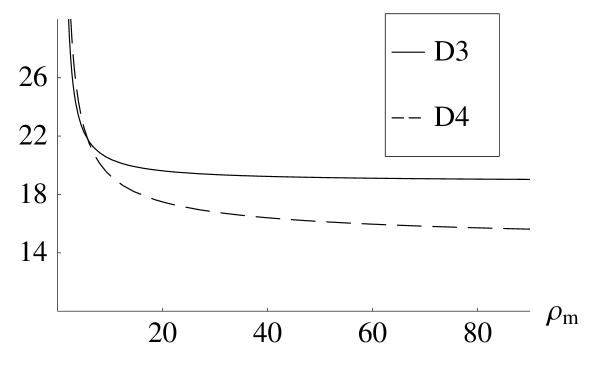
Plotting $\hat{q}$ as a function of the mass of the quarks, we observe a very weak dependence until the mass is rather low, where the approximations are questionable. For example, for the case of the D3 background, the horizontal axis is $\rho_{m}=m/(2\pi^{3/2}\sqrt{\alpha_{SYM}N_{c}}T)\simeq m/2.7$ GeV for $\alpha_{SYM}=1/2,N_{c}=3$ and $T=200$ MeV. In order to increase $\hat{q}$ by a 10$\%$ we must lower $\rho_{m}$ until a value of $\simeq 10$, hence $m\simeq 27$ GeV.

3 $\hat{q}$ at finite coupling

The AdS/CFT correspondence is a statement that goes beyond the classical limit of string theory. In this limit, it maps classical solutions of supergravity to quantum field theory vacua in the strong coupling limit, $\lambda\to\infty$. Corrections in $\lambda^{-1}$ are in direct correspondence with those in powers of $\alpha^{\prime}$ in the string theory side. In this paper we shall use the solution given in [23, 30] corresponding to the $\alpha^{\prime}$ corrected near extremal D3–brane. The relevant pieces of information of this solution can be casted as follows

$$\hat{c}_{T}^{2}(\rho) = \rho^{2}(1-\rho^{-4})(1+\gamma\,T(\rho)+...)\,,$$

$$\hat{c}_{X}^{2}(\rho) = \rho^{2}(1+\gamma\,X(\rho)+...)\,,$$

$$\hat{c}_{R}^{2}(\rho) = \rho^{-2}(1-\rho^{-4})^{-1}\,(1+\gamma\,R(\rho)+...)~{},$$

to first order in $\gamma=\frac{\zeta(3)}{8}\,(\alpha^{\prime}/R^{2})^{3}\sim 0.15\,\lambda^{-3/2}$. Here, following (15), we have already extracted $\Delta_{R}=R^{2}/r_{H}^{2}$ factors, with $R^{2}=\sqrt{\lambda}\,\alpha^{\prime}$. The intervening functions read

$$T(\rho) = \left(-75\rho^{-4}-\frac{1225}{16}\rho^{-8}+\frac{695}{16}\rho^{-12}\right)\,,$$

$$X(\rho) = \left(-\frac{25}{16}\rho^{-8}(1+\rho^{-4})\right)\,,$$ (21)

$$R(\rho) = \left(75\rho^{-4}+\frac{1175}{16}\rho^{-8}-\frac{4585}{16}\rho^{-12}\right)\,.$$

Inserting this data in (19) with $p=3$ and expanding to first order in $\gamma$ gives

$$\hat{q}(\lambda)=\hat{q}(0)\left(1-\gamma\left[\frac{I}{2a}+45\right]+...\right)$$ (22)

with $\hat{q}(0)$ as given in [16], and

$$a = \int_{1}^{\infty}\frac{d\rho}{\sqrt{\rho^{4}-1}}=\sqrt{\pi}\,\frac{\Gamma\left(5/4\right)}{\Gamma\left(3/4\right)}~{},$$ (23)

$$I = \int_{1}^{\infty}\frac{R(\rho)-X(\rho)\,(\rho^{4}+2)+T(\rho)\,(\rho^{4}-1)}{\sqrt{\rho^{4}-1}}d\rho=-\frac{30725\,\pi^{3/2}}{924\sqrt{2}\,\Gamma\left(3/4\right)^{2}}~{}.$$ (24)

Evaluating yields

$$\hat{q}(\lambda)=\hat{q}(0)\left(1-1.7652\,\lambda^{-3/2}+\dots\right).$$ (25)

Therefore, we see that finite coupling corrections tend to diminish the value of the quenching parameter. For example, taking $N_{c}=3$ and $\alpha_{SYM}=1/4$, $1/2$ and $1$, we get a reduction factor of $6,$ $2$ and $0.8$ percent respectively. Note that the decrease in the jet quenching parameter towards weak coupling is suggestive of a smooth interpolation between the strong coupling regime and the perturbative results. Obviously, the computation of higher order corrections would be necessary to put this conclusion on more solid grounds.

4 $\hat{q}$ at finite chemical potential

The near horizon metric of a rotating black D3–brane with maximal number of angular momenta reads as follows [31, 32], with the conventions of [33]:

$$ds^{2}=\sqrt{\Delta}\left(-{\cal H}^{-1}fdt^{2}+f^{-1}dr^{2}+\frac{r^{2}}{R^{2}}\,d\vec{x}\cdot d\vec{x}\right)+\frac{1}{\sqrt{\Delta}}\sum_{i=1}^{3}R^{2}H_{i}\left[d\nu_{i}^{2}+\nu_{i}^{2}(d\phi_{i}+A^{i}dt)^{2}\right]~{},$$ (26)

where $\nu_{1}=\cos\theta_{1},~{}\nu_{2}=\sin\theta_{1}\cos\theta_{2},~{}\nu_{3}=\sin\theta_{1}\sin\theta_{2}$, and ${\cal H}=H_{1}H_{2}H_{3}$, where

$$A^{i}=\frac{1}{R}\sqrt{\frac{\mu}{q_{i}}}(1-H_{i}^{-1})~{},\qquad H_{i}=1+\frac{q_{i}}{r^{2}}~{},\qquad f=\frac{r^{2}}{R^{2}}{\cal H}-\frac{\mu}{r^{2}}~{},\qquad\Delta={\cal H}\sum_{i=1}^{3}\frac{\nu_{i}^{2}}{H_{i}}~{}.$$ (27)

Upon Kaluza-Klein reduction, this becomes a charged AdS black hole solution of $\mathcal{N}=2$ $U(1)_{R}^{3}$ supergravity, where $A^{i}$ plays the rôle of the gauge field. The holographic gauge theory corresponding to (26) is $\mathcal{N}=4$ $SU(N)$ supersymmetric Yang-Mills at finite temperature and with a chemical potential for the $U(1)_{R}^{3}$ symmetry. It will be convenient to trade the nonextremality parameter $\mu$ for the horizon radius, $r=r_{H}$ given as the largest root of $f(r_{H})=0$, i.e.,

$$\mu=\frac{r_{H}^{4}}{R^{2}}\,{\cal H}(r_{H})\,,$$ (28)

and define the adimensional quantities

$$\kappa_{i}=\frac{q_{i}}{r_{H}^{2}}~{},\qquad\Delta_{R}=\frac{R^{2}}{r_{H}^{2}}~{}.$$ (29)

As usual, we go to dimensionless variable $\rho=r/r_{H}$ and find

$$H_{i}(\rho)=1+\kappa_{i}\rho^{-2}~{},\qquad f(\rho)=\frac{1}{\Delta_{R}}\left(\rho^{2}{\cal H}(\rho)-\rho^{-2}{\cal H}(1)\right)\equiv\frac{1}{\Delta_{R}}\hat{f}(\rho)~{}.$$ (30)

Finally, the relevant functions entering the formula (16) can be easily extracted from (26):

$$\hat{c}_{T}^{2}(\rho)=\frac{\sqrt{\Delta}\,\hat{f}}{{\cal H}}-\frac{1}{\sqrt{\Delta}}\sum_{i=1}^{3}\frac{\nu_{i}^{2}\,{\cal H}(1)}{\kappa_{i}H_{i}}(H_{i}-1)^{2}~{},\qquad\hat{c}_{X}^{2}(\rho)=\sqrt{\Delta}\,\rho^{2}~{},\qquad\hat{c}_{R}^{2}(\rho)=\frac{\sqrt{\Delta}}{\hat{f}}~{}.$$ (31)

The factors in the metric depend on the internal angles. However, the terms above conspire to give

$$\int_{1}^{\infty}\frac{\hat{c}_{R}d\rho}{\hat{c}_{X}^{2}\sqrt{\hat{c}_{X}^{2}-\hat{c}_{T}^{2}}}=\frac{1}{{\cal H}(1)}\int_{1}^{\infty}d\rho\left(\rho^{4}\frac{{\cal H}(\rho)}{{\cal H}(1)}-1\right)^{-1/2}~{},$$ (32)

where all information about the internal angular coordinates has dissapeared. Now, given that the Hawking temperature of this solution is given by [31]

$$T=\frac{2+\sum_{i=1}^{3}\kappa_{i}-\prod_{i=1}^{3}\kappa_{i}}{2\sqrt{{\cal H}(1)}}~{}\frac{r_{H}}{\pi R^{2}}$$ (33)

with $R^{2}=\sqrt{\lambda}\,\alpha^{\prime}$, substituting in (16) we find the answer

$$\hat{q}(\kappa_{i})=\frac{\pi^{2}T^{3}\sqrt{\lambda}}{\sqrt{2}}\,{\cal H}(1)\,\left(\frac{2\sqrt{{\cal H}(1)}}{2+\sum_{i=1}^{3}\kappa_{i}-\prod_{i=1}^{3}\kappa_{i}}\right)^{3}\left(\int_{1}^{\infty}d\rho\left(\rho^{4}\frac{{\cal H}(\rho)}{{\cal H}(1)}-1\right)^{-1/2}\right)^{-1}.$$ (34)

In order to analyze this result, it must be recalled that the domain of thermodynamical stability of this solution [34, 35] (see also [36]) is bounded by the inequality $\kappa_{1}+\kappa_{2}+\kappa_{3}-\kappa_{1}\,\kappa_{2}\,\kappa_{3}<2$.

Figure 2: Plot of $\hat{q}$ as function of different combinations of charges $\kappa_{i}$. The charges which are not varied are set equal to zero. The stability bound chops the lower curves, but leaves the upper one unbounded. At the origin the value is $\simeq 18.87$ as found in LRW.

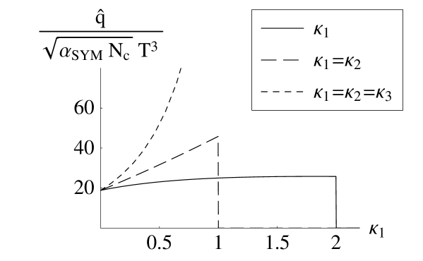
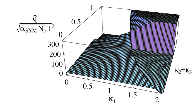
Plotting the right hand side of (34) numerically, we find the curves that are shown in figure 2. The jet quenching parameter raises its value for nonzero charges. The increase is not monotonous along the whole space of charges. In fact, though hardly noticeable, it changes the sign of the slope along the line $\kappa_{1}$ with $\kappa_{2}=\kappa_{3}=0$. To see this better, we have zoomed the interval $\kappa_{1}\in[1.4,2]$ in figure 3, where we can see that the change in slope sign happens around $\kappa_{1}=1.8$.

Figure 3: Zoom of the curve $\hat{q}(\kappa_{1})$ showing the value of the turning and end points.

A comparison with recent results in the literature is in order. We certainly agree and go beyond the perturbative analysis of Cáceres and Guijosa [19]. Also, when restricted to the cases examined by Lin and Matsuo [20] (one charge) and Avramis and Sfetsos [21] (one or two equal charges), we find qualitative agreement within the range of stability. We may also examine less symmetrical configurations on a 3 dimensional plot in figure 4.

Figure 4: Evolution of $\hat{q}$ in a sector of the plane $(\kappa_{1},\kappa_{2}=\kappa_{3})$. The curve is chopped by the thermodynamical stability bound.

Besides analyzing the qualitative behaviour of $\hat{q}(\kappa_{i})$ numerically, in order to compare with other approaches, it may be of interest to perform an expansion in powers of quantum field theoretical magnitudes. For this purpose, it is relevant to recall how the thermodynamical magnitudes are related to geometrical quantities. In particular, the density of physical charge and chemical potential are given respectively by [35, 37]

$$\rho_{i} = \frac{\pi N^{2}T_{0}^{3}}{8}\sqrt{2\kappa_{i}}\,\prod_{i=1}^{3}(1+\kappa_{i})^{1/2}~{},$$ (35)

$$\mu_{i} \equiv \left.A^{i}(r)\right|_{r=r_{H}}=\frac{\pi T_{0}\sqrt{2\kappa_{i}}}{1+\kappa_{i}}\prod_{i=1}^{3}(1+\kappa_{i})^{1/2}~{},$$ (36)

where $T_{0}=r_{H}/(\pi R^{2})$. From these expressions and (33), we should invert $\kappa_{i}$ in terms of $\rho_{i}$ and $T$ for the canonical ensemble and in terms of $\mu_{i}$ and $T$ for the grand canonical ensemble. This is dificult in the general case, so we may simplify for equal or vanishing values of $\kappa_{i}$. For example, taking $\kappa_{1}=\kappa$ and $\kappa_{2}=\kappa_{3}=0$ the two (inverse) expansions yield

$$\kappa_{C} = \xi-\xi^{2}+\frac{11}{4}\xi^{3}+...~{},$$ (37)

$$\kappa_{GC} = \zeta+\zeta^{2}+\frac{5}{4}\zeta^{3}+...~{},$$ (38)

with

$$\xi=\left(\frac{4\sqrt{2}\rho}{\pi N^{2}T^{3}}\right)^{2}~{},~{}~{}~{}~{}~{}~{}~{}~{}~{}~{}~{}\zeta=\left(\frac{\mu}{\sqrt{2}\pi T}\right)^{2}~{}.$$ (39)

Expanding (34) in powers of $\kappa$ and inserting these series we obtain for the canonical and grand-canonical ensemble respectively the following results

$$\hat{q}_{C}(\rho) = \hat{q}(0)\left(1+0.63\,\xi-1.08\,\xi^{2}+2.83\xi^{3}+...\right)~{},$$ (40)

$$\hat{q}_{GC}(\mu) = \hat{q}(0)\left(1+0.63\,\zeta+0.18\,\zeta^{2}+0.06\zeta^{3}+...\right)~{}.$$ (41)

This expansion fully agrees with the one in [21] upon rescaling $\xi\to 2\xi^{2}$ and $\zeta\to 2\hat{\xi}^{2}$.

The computation of Wilson loops in thermal $AdS$ backgrounds is a promising line of research, of which the $\hat{q}$ computation is a salient example. The identification of other observables within the AdS/CFT framework (see, for a recent example, [38]) that can be confronted with experimental data is an urget challenge. It seems clear to us that there are several avenues for further exploration. Among these, the extension of our results to less supersymmetric backgrounds is of neat interest. We hope to report on these issues in the near future.

References

- [1] K. Adcox et al. [PHENIX Collaboration], Nucl. Phys. A 757, 184 (2005). B. B. Back et al., Nucl. Phys. A 757, 28 (2005). I. Arsene et al. [BRAHMS Collaboration], Nucl. Phys. A 757, 1 (2005). J. Adams et al. [STAR Collaboration], Nucl. Phys. A 757, 102 (2005).
- [2] R. Baier, Y. L. Dokshitzer, A. H. Mueller, S. Peigne and D. Schiff, Nucl. Phys. B 484, 265 (1997).
- [3] R. Baier, D. Schiff and B. G. Zakharov, Ann. Rev. Nucl. Part. Sci. 50, 37 (2000). M. Gyulassy, I. Vitev, X. N. Wang and B. W. Zhang, arXiv:nucl-th/0302077.
- [4] A. Kovner and U. A. Wiedemann, arXiv:hep-ph/0304151.
- [5] B. G. Zakharov, JETP Lett. 65, 615 (1997). U. A. Wiedemann, Nucl. Phys. B 588, 303 (2000). M. Gyulassy, P. Levai and I. Vitev, Nucl. Phys. B 594, 371 (2001). X. N. Wang and X. f. Guo, Nucl. Phys. A 696, 788 (2001). S. Jeon and G. D. Moore, Phys. Rev. C 71, 034901 (2005).
- [6] I. Vitev, arXiv:hep-ph/0603010. K. J. Eskola, H. Honkanen, C. A. Salgado and U. A. Wiedemann, Nucl. Phys. A 747, 511 (2005). A. Dainese, C. Loizides and G. Paic, Eur. Phys. J. C 38, 461 (2005). M. Djordjevic, M. Gyulassy, R. Vogt and S. Wicks, Phys. Lett. B 632, 81 (2006). N. Armesto, M. Cacciari, A. Dainese, C. A. Salgado and U. A. Wiedemann, Phys. Lett. B 637, 362 (2006).
- [7] N. Armesto, C. A. Salgado and U. A. Wiedemann, Phys. Rev. Lett. 93, 242301 (2004). T. Renk and J. Ruppert, Phys. Rev. C 72, 044901 (2005).
- [8] A. Adil, M. Gyulassy, W. A. Horowitz and S. Wicks, arXiv:nucl-th/0606010.
- [9] F. Arleo, Eur. Phys. J. C 30, 213 (2003).
- [10] R. Baier, Nucl. Phys. A 715, 209 (2003).
- [11] J. M. Maldacena, Adv. Theor. Math. Phys. 2, 231 (1998) [Int. J. Theor. Phys. 38, 1113 (1999)].
- [12] E. Witten, Adv. Theor. Math. Phys. 2, 505 (1998).
- [13] S. J. Rey and J. T. Yee, Eur. Phys. J. C 22, 379 (2001). J. M. Maldacena, Phys. Rev. Lett. 80, 4859 (1998). S. J. Rey, S. Theisen and J. T. Yee, Nucl. Phys. B 527, 171 (1998).
- [14] G. Policastro, D. T. Son and A. O. Starinets, JHEP 0209, 043 (2002). G. Policastro, D. T. Son and A. O. Starinets, JHEP 0212, 054 (2002).
- [15] G. Policastro, D. T. Son and A. O. Starinets, Phys. Rev. Lett. 87, 081601 (2001). A. Buchel and J. T. Liu, Phys. Rev. Lett. 93, 090602 (2004).
- [16] H. Liu, K. Rajagopal and U. A. Wiedemann, arXiv:hep-ph/0605178.
- [17] A. Buchel, arXiv:hep-th/0605178.
- [18] J. F. Vazquez-Poritz, arXiv:hep-th/0605296.
- [19] E. Caceres and A. Guijosa, arXiv:hep-th/0606134.
- [20] F. L. Lin and T. Matsuo, arXiv:hep-th/0606136.
- [21] S. D. Avramis and K. Sfetsos, arXiv:hep-th/0606190.
- [22] C. P. Herzog, A. Karch, P. Kovtun, C. Kozcaz and L. G. Yaffe, arXiv:hep-th/0605158. J. Casalderrey-Solana and D. Teaney, arXiv:hep-ph/0605199. S. S. Gubser, arXiv:hep-th/0605182. C. P. Herzog, arXiv:hep-th/0605191. E. Caceres and A. Guijosa, arXiv:hep-th/0605235. J. J. Friess, S. S. Gubser and G. Michalogiorgakis, arXiv:hep-th/0605292. S. J. Sin and I. Zahed, arXiv:hep-ph/0606049.
- [23] S. S. Gubser, I. R. Klebanov and A. A. Tseytlin, Nucl. Phys. B 534, 202 (1998).
- [24] A. Buchel, J. T. Liu and A. O. Starinets, Nucl. Phys. B 707, 56 (2005).
- [25] M. Kruczenski, D. Mateos, R. C. Myers and D. J. Winters, JHEP 0405, 041 (2004).
- [26] N. Itzhaki, J. M. Maldacena, J. Sonnenschein and S. Yankielowicz, Phys. Rev. D 58, 046004 (1998).
- [27] A. Karch and E. Katz, JHEP 0206, 043 (2002).
- [28] M. Kruczenski, D. Mateos, R. C. Myers and D. J. Winters, JHEP 0307, 049 (2003).
- [29] H. Dorn and H. J. Otto, JHEP 9809, 021 (1998). S. Forste, D. Ghoshal and S. Theisen, JHEP 9908, 013 (1999). J. Greensite and P. Olesen, JHEP 9904, 001 (1999).
- [30] J. Pawelczyk and S. Theisen, JHEP 9809, 010 (1998).
- [31] J. G. Russo and K. Sfetsos, Adv. Theor. Math. Phys. 3, 131 (1999).
- [32] M. Cvetic et al., Nucl. Phys. B 558, 96 (1999).
- [33] A. Buchel, arXiv:hep-th/0604167.
- [34] M. Cvetic and S. S. Gubser, JHEP 9904, 024 (1999).
- [35] D. T. Son and A. O. Starinets, JHEP 0603, 052 (2006).
- [36] R. G. Cai and K. S. Soh, Mod. Phys. Lett. A 14, 1895 (1999). T. Harmark and N. A. Obers, JHEP 0001, 008 (2000).
- [37] J. Mas, JHEP 0603, 016 (2006).
- [38] K. Peeters, J. Sonnenschein and M. Zamaklar, arXiv:hep-th/0606195.