Soliton solutions of the improved quark mass density-dependent model at finite temperature

Abstract

The improved quark mass density-dependent model (IQMDD) based on soliton bag model is studied at finite temperature. Appling the finite temperature field theory, the effective potential of the IQMDD model and the bag constant $B(T)$ have been calculated at different temperatures. It is shown that there is a critical temperature $T_{C}\simeq 110\mathrm{MeV}$. We also calculate the soliton solutions of the IQMDD model at finite tmperature. It turns out that when $T<T_{C}$, there is a bag constant $B(T)$ and the soliton solutions are stable. However, when $T>T_{C}$ the bag constant $B(T)=0$ and there is no soliton solution, therefore, the confinement of quarks are removed quickly.

I Introduction

It is widely believed that the fundamental theory of strong interaction is quantum chromodynamics (QCD), which in principle can be applied to describe most of nuclear physics. However, due to the property of confinement and asymptotic freedom, QCD can not yet be used to study low-energy nuclear physics. The challenge to nuclear physicists is to find models which can bridge the gap between the fundamental theory and our wealth of knowledge about low energy phenomenology. Some of these models have been proved to be successful in reproducing different properties of hadrons, nuclear matter and quark matter Serot:1997xg ; Tomas:1984 ; Farhi:1984qu ; Madsen:1989pg ; Greiner:1987tg ; Fowler:1981rp . The quark mass density-dependent model (QMDD) is one of such candidates.

The QMDD model was first suggested by Fowler, Raha and Weiner Fowler:1981rp , and then employed by many authors to study the stability and physical properties of strange quark matter Chakrabarty:1991ui ; Benvenuto:1989kc ; Peng:2000ff ; Wang:2000dc . This model provides an alternative phenomenological description of quark confinement because in this model, the mass of quarks is given by

$$m_{u,d} = \frac{B}{n_{q}},$$ (1)

$$m_{s} = m_{s0}+\frac{B}{n_{q}},$$ (2)

where $B$ is the vacuum energy density and $n_{q}=n_{u}+n_{d}+n_{s0}$. $n_{u},n_{d},n_{s0}$ represent the number density of the $u,d$ and $s$ quarks respectively. We see from Eqs.(1), (2), if the distance between quarks goes to infinity, the volume of the system becomes infinite, $n_{q}$ approaches to zero and $m_{q}$ ($q=u,d,s$) approaches to infinite. This is just the confinement condition as that of MIT bag model Tomas:1984 . However, QMDD model has its advantage since the boundary condition put by hand in MIT model to confine quarks is abandoned. This correspondence was confirmed by Benvenuto and Lugones Benvenuto:1989kc . They proved that the properties of strange matter in the QMDD model are nearly the same as those obtained in the MIT bag model.

Although the QMDD model can provide a dynamical description of confinement and explain the stability and many other dynamical properties of strange quark matter (SQM) at zero temperature, there are many difficulties when we extend this model to finite temperature. They are: 1) it cannot mimic the correct ”temperature $T$ vs. density $\rho$” deconfinement phase diagram of QCD because the quark masses are divergent and then $T$ tends to infinite when $n_{q}\to 0$ Zhang:2002fs ; 2) Although the basic improvement of QMDD model is the quark masses depending on density and the quark confinement mechanism mimics, it is still an ideal quark gas model with no quark-quark interaction included. However, as was shown in recent RHIC experiments, the quark-quark interaction cannot be neglected in Quark-Gluon plasma. In order to overcome the first difficulty, a quark mass density- and temperature dependent (QMDTD) model Zhang:2002fs ; Zhang:2002qq ; Zhang:2003ka ; Zhang:2003fn ; Zhang:2001ih is proposed and it was argued that $B$ is a function of temperature as that of Friedberg-Lee (FL) model Friedberg:1976eg ; Birse:1991cx ; Wilets:1990di . The equation of state of QMDTD model are used to study the properties of strange quark star in Refs.Gupta:2002hj Shen:2005vh and the results are successful. To the second difficulty, as a first step, Ref.Wu:2005ty has introduced a coupling between quark and non-linear scalar field to improve the QMDD model and have investigated the properties of nucleon successfully. Instead of the correspondence of MIT bag to QMDD model, a FL soliton bag is formed by quark and scalar field coupling for improved QMDD (IQMDD) model and the quark deconfinement phase transition can take place.

This paper evolves from an attempt to extend the IQMDD model Wu:2005ty to finite temperature. Since the spontaneously broken symmetry of the scalar field will be restored at finite temperature, the non-topological soliton tends to disappear when temperature $T$ increases to $T_{C}$. If the temperature increases further, the solution becomes a damping oscillation and such a solution can not be taken as ”soliton ” solution, so the quarks are to be deconfined.

By using the finite temperature field theory, we will calculate the effective potential under one-loop approximation and find $T_{C}\approx 110\mathrm{MeV}$. Studying the temperature dependence of soliton solutions is our first motivation. Our second motivation is to find the function $B(T)$. In QMDTD model, $B(T)$ is an input. As an ansatz, two formulae

$$B_{1}(T)=B_{0}[1-A_{1}(\frac{T}{{T_{C}}})+A_{2}(\frac{T}{{T_{C}}})^{2}],\quad 0\leq T\leq T_{C}$$ (3)

with $A_{1},A_{2}$ adjustable parameters, and

$$B_{2}(T)=B_{0}[1-(\frac{T}{{T_{C}}})^{2}],\quad 0\leq T\leq T_{C}$$ (4)

were introduced in Ref.Zhang:2001ih and Ref.Zhang:2002fs respectively. However, for FL model or for the IQMDD model, $B(T)$ can be calculated because the vacuum energy density $B$ equals the difference of the value of the effective potential between the vacua inside and outside the soliton bag, and the vacua of the effective potential depend on temperature.

The organization of this paper is as follows. In the following section we review the IQMDD model and its numerical solutions for our selected parameters. In Sec.III, we give detailed calculation of the effective potential of the IQMDD model and the bag constant as functions of temperature. The soltion solutions of the IQMDD model at different temperatures are presented in Sec.IV, while in the last section we present our summary and discussion.

II The IQMDD model

Since the details of IQMDD model can be found in Ref.Wu:2005ty , hereafter we only write down the essential formulae which are necessary for our further discussion. The effective Lagrangian density of the IQMDD model is Wu:2005ty

$$\mathcal{L}=\overline{\psi}(i\eth-g\sigma-m_{q})\psi+\frac{1}{2}\partial_{\mu}\sigma\partial^{\mu}\sigma-U(\sigma),$$ (5)

which describes the interaction of the spin-$\frac{1}{2}$ quark fields $\psi$ and the phenomenological scalar field $\sigma$ with the coupling constant $g$. $m_{q}$ is the mass of u(d) quark, which is given by Eq.(1). In this paper we do not discuss the strange quark. The potential for the $\sigma$ field is chosen as

$$U(\sigma)=\frac{a}{2!}\sigma^{2}+\frac{b}{3!}\sigma^{3}+\frac{c}{4!}\sigma^{4}+B,$$ (6)

$$b^{2}>3ac$$ (7)

The condition (7) ensures that the absolute minimum of $U(\sigma)$ is at $\sigma=\sigma_{v}\neq 0$.

$U(\sigma)$ has two minima: one is the absolute minimum at a large value of the $\sigma$ field

$$\sigma_{v}=\frac{3|b|}{2c}\left[1+\left[1-\frac{8ac}{3b^{2}}\right]^{\frac{1}{2}}\right],$$ (8)

with $U(\sigma_{v})=0$, another is at $\sigma_{0}=0$. The former corresponds to the physical or nonperturbative vacuum, and $\sigma=\sigma_{v}$ representing some condensates. The other represents a metastable vacuum where the condensates vanishes, with an energy density $B$ relative to the physical vacuum. The ”bag constant” $B$ can be expressed as

$$-B=\frac{a}{2!}\sigma^{2}_{v}+\frac{b}{3!}\sigma^{3}_{v}+\frac{c}{4!}\sigma^{4}_{v}.$$ (9)

From Eq.(5), the classical Euler-Lagrangian equations can be obtained as

$$(i\eth-g\sigma-m_{q})\psi = 0,$$ (10)

$$\square\sigma+\frac{dU}{d\sigma}+g\overline{\psi}\psi = 0.$$ (11)

In the mean-field approximation (MFA), the scalar field $\sigma$ is taken as time-independent classical c-number field, and we only consider a fixed occupation number of valence quarks (3 quarks for nucleons, and quark-antiquark pair for mesons). Quantum fluctuation of the bosons and effects of the quark Dirac sea are thus to be neglected. In the following , we will discuss the ground state solution of the system.

In the spherical case, the $\sigma$ is spherically symmetric, and valence quarks are in the lowest s-wave level. Then the scalar field $\sigma$ and the Dirac equation functions can be written as

$$\sigma(\mathbf{r},t) = \sigma(r),$$ (12)

$$\psi(\mathbf{r},t) = e^{-i\epsilon t}\sum_{i}\varphi_{i},$$ (13)

where the quark Dirac spinors have the form

$$\varphi=\left(\begin{array}[]{c}u(r)\\ i\vec{\sigma}\cdot\mathbf{\hat{r}}v(r)\end{array}\right)\chi.$$ (16)

By using Eqs.(10)-(16), we obtain

$$\frac{du(r)}{dr}=-(\epsilon+m_{q}+g\sigma(r))v(r),$$ (17)

$$\frac{dv(r)}{dr}=-\frac{2}{r}v(r)+(\epsilon-m_{q}-g\sigma(r))u(r),$$ (18)

$$\frac{d^{2}\sigma(r)}{dr^{2}}+\frac{2}{r}\frac{d\sigma(r)}{dr}-\frac{dU}{d\sigma}=Ng(u^{2}(r)-v^{2}(r)).$$ (19)

The quark functions should satisfy the normalisation condition

$$4\pi\int r^{2}(u^{2}(r)+v^{2}(r))dr=1.$$ (20)

The number of quarks would be $N=3$ for baryons and $N=2$ for mesons. In the following discussions, we only constrain in the case $N=3$. These equations are subject to the boundary conditions which follow from the requirement of finite energy:

$$v(0)=0,\frac{d\sigma(0)}{dr}=0,$$

$$u(\infty)=0,\sigma(\infty)=\sigma_{v}.$$

If we consider $N$ quarks in the lowest mode with energy $\epsilon$, the total energy of the system is

$$E=N\epsilon+4\pi\int r^{2}\left[\frac{1}{2}\left(\frac{d\sigma}{dr}\right)^{2}+U(\sigma)\right]dr.$$ (21)

This model has four adjustable parameter $g,a,b,c$ which can be chosen to fit various baryon properties such as the proton change radius $r_{cp}$, the proton magnetic moment $\mu_{p}$ and the ratio of axial-vector to vector coupling $g_{A}/g_{v}$. In Ref.Wu:2005ty , a wide rage of parameters has been used to calculate above quantities. Hereafter we take one set of parameters $a=70.0fm^{-2}$, $b=-2201.8fm^{-1}$, $c=20000$ and $g=9.8$ to study the temperature dependence of the soliton solution. It has been proven in Ref.Wu:2005ty that this set of parameters can describe the properties of nucleon at zero temperature successfully.

Figure 1: The $\sigma$ and quark fields in arbitrary unit as functions of r for the parameters taken as $a=70.0fm^{-2}$, $b=-2201.8fm^{-1}$, $c=20000$ and $g=9.8$.

Figure 2: The quark density $u^{2}(r)-v^{2}(r)$ in arbitrary unit as functions of r for the parameters taken as $a=70.0fm^{-2}$, $b=-2201.8fm^{-1}$, $c=20000$ and $g=9.8$.

In Fig.1 we plot the $\sigma$ and quark fields profiles in arbitrary unit as functions of r for the above parameters. The quark density $u^{2}(r)-v^{2}(r)$ distribution versus radius are plotted in Fig.2.

III Effective potential at finite temperature

The appropriate framework for studying phase transitions is finite temperature field theory or thermal field theory. Within this framework the finite temperature effective potential is an important and useful theoretical tool. The idea of such techniques could trace back to the 1970’s when Kirzhnits and Linde first proposed that symmetries broken at zero temperature could be restored at finite temperatureKirzhnits:1972iw Kirzhnits:1972ut . Subsequently WeinbergWeinberg:1974hy , Dolan and Jackiw Dolan:1973qd as well as many others have adopted the effective potential as the basic tool to study the symmetry-breaking phase transitions. In this section we briefly outline the relevant results of Dolan and JackiwDolan:1973qd , since the IQMDD model is very similar to the model studied by those authors.

The effective potential can be calculated to one-loop order by using the methods of Dolan and JackiwDolan:1973qd . But it is pointed out in RefFriedberg:1976eg ; Lee:1981mf that, as an approximation, all $\sigma$ quantum loop diagrams may be ignored due to the fact that $\sigma$ is only a phenomenological field describing the long-range collective effects of QCD, its short-wave components do not exist in reality. Therefore for the rest of this discussion we shall ignore quantum corrections and concentrate on those induced by finite temperature effects. Then the one-loop contribution to the effective potential is of the form

$$V(\sigma;\beta)=U(\sigma)+V_{B}(\sigma;\beta)+V_{F}(\sigma;\beta),$$ (22)

where $U(\sigma)$ is the classical potential of the Lagrangian. $V_{B}(\sigma;\beta)$ and $V_{F}(\sigma;\beta)$ are the finite temperature contributions from boson and fermion one-loop diagrams respectivelyDolan:1973qd Das:1997gg . It should be pointed out that, in this approximate method for the calculation of the effective potential, the plane wave quark states have been used, while, in fact, the quarks are confined in the finite-size solitonic configuration. Therefore, this approximate method is not fully self-consistent. For simplicity, we have substituted $\sigma(T)$ for $\bar{\sigma}(T)$. These contribute the following terms in the potentialDolan:1973qd

$$V_{B}(\sigma;\beta)=\frac{1}{2\pi^{2}\beta^{4}}\int^{\infty}_{0}dxx^{2}\mathrm{ln}\left(1-e^{-(x^{2}+\beta^{2}m_{\sigma}^{2})}\right),$$ (23)

$$V_{F}(\sigma;\beta)=-12\sum_{n}\frac{1}{2\pi^{2}\beta^{4}}\int^{\infty}_{0}dxx^{2}\mathrm{ln}\left(1+e^{-(x^{2}+\beta^{2}m_{qn}^{2})}\right),$$ (24)

where the minus sign is the consequence of Fermi-Dirac statistics. $m_{\sigma}$ and $m_{q}$ are the effective masses of the scalar field $\sigma$ and the quark field, respectively:

$$m_{q} = \frac{B(T)}{n_{q}}+g\sigma(T),$$ (25)

$$m^{2}_{\sigma} = a+b\sigma(T)+\frac{c}{2}\sigma^{2}(T).$$ (26)

We fix $m^{2}_{\sigma}$ by taking its value at the physical vacuum stateGao:1992zd . In this work, $B(T)$ is defined as the difference between the vacua of the effective potential inside and outside the solion bag. This means that for $T\leq T_{C}$, $B(T)$ is the difference between the effective potential values at the perturbative vacuum state and values at the physical vacuum state

$$B(T)=V(\sigma_{0};\beta)-V(\sigma_{v};\beta).$$ (27)

For $T>T_{C}$, $B(T)=0$ due the fact that the vacua inside and outside the soliton bag are equal. This will be analyzed in more details in next section.

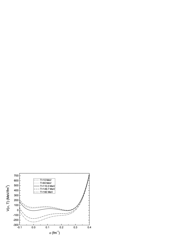
Figure 3: The temperature-dependence of the one-loop effective potential $V(\sigma;\beta)$. At low temperature, there are two minima and one of which is going to disappear when the temperature reaching a high temperature $T=149.7\mathrm{MeV}$. The critical temperatures is set at $T_{C}\simeq 110\mathrm{MeV}$ when two minima are euqal.

From Eqs.(22), (25) and (26), we can numerically solve the effective potential $V(\sigma;\beta)$ for different temperatures. In Fig.3, we plot the one-loop effective potential $V(\sigma;\beta)$ as a function of $\sigma$ at $T=10\mathrm{MeV}$, $T=80\mathrm{MeV}$, $T=110.0\mathrm{MeV}$, $T=149.7\mathrm{MeV}$ and $T=160\mathrm{MeV}$. It can be seen from Fig.3 that there exist two particular temperatures. One is that the effective potential exhibits two degenerate minima at $T_{C}\simeq 110\mathrm{MeV}$ which is defined as critical temperature, the other is that the second minimum of the potential at $\sigma\simeq\sigma_{v}$ disappears at a higher temperature $T\simeq 149.7\mathrm{MeV}$.

For low temperatures the absolute minimum of $V(\sigma;\beta)$ lies close to $\sigma_{v}$, and there is another minimum at $\sigma_{0}$. The physical vacuum state at $\sigma_{v}$ is stable and correspondingly quarks are in confinement. As the temperature increases the second minimum of the potential at $\sigma_{0}$ decreases relative to the first one. At the critical temperature $T_{C}\simeq 110\mathrm{MeV}$, the potentials at the two minima are equal. The physical vacuum becomes unstable. Since $B(T)=0$ when $T$ is lager than $T_{C}$, there is no bag constant to provide the dynamical mechanism to confine the quarks in the bag. Moreover, there is no soliton-like solution in the model when the temperature is above $T_{C}$ due to the effective potential and vacuum structure, there only exists the damping oscillation solution and such a solution can not produce a mechanism to confine the quarks in a small region, we will investigate the damping oscillation in next section more detail. Therefore as the temperature is above $T_{C}$, the confinement of the quarks is removed completely.

Figure 4: The bag constant $B(T)$ as functions of $T$.

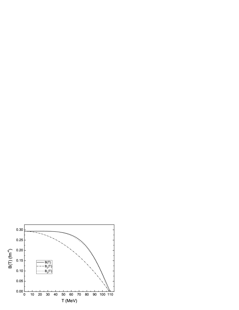
Figure 5: The bag constant $B(T)$, $B_{2}(T)$ and $B_{3}(T)$as functions of $T$.

Using the obtained temperature-dependent effective potentials, from Eq.(27) we illustrate the temperature dependence of the bag constant $B(T)$ in Fig.4, and it is shown that the bag constant decreases continuously with increasing temperature. At the critical temperature $T_{C}$, $B(T_{C})=0$. We can fit the analytical formula of the bag constant as a function of $T$

$$B_{3}(T)=B_{0}\left[1-c1\left(\frac{T}{T_{C}}\right)^{2}-c2\left(\frac{T}{T_{C}}\right)^{4}\right],$$ (28)

where $B_{0}$ is the bag constant at zero temperature, the parameters are $c1=-0.113$ and $c2=1.113$ respectively. For comparison, we plot $B(T)$, $B_{2}(T)$ of Eq.(4) and $B_{3}(T)$ in Fig.5. $B_{2}(T)$ decreases smoothly with increasing temperature, while $B(T)$ and $B_{3}(T)$ decrease dramatically with increasing temperature when the temperature is around $85\mathrm{MeV}$. From Eq.(3), we can give the parameters $A_{1}\simeq-0.67$ and $A_{2}\simeq 1.55$.

IV The soliton solutions and deconfinement phase transtions

Soliton models such as those described in Section II can be modified so as to allow for the effect of thermal background with temperature $\beta$, just by replacing the relevant classical potential function $U(\sigma)$ by an appropriately modified temperature-dependent effective potential $V(\sigma;\beta)$Holman:1992rv Carter:2002te .

For finite temperature soliton solutions will take the same form as the one at zero temperature. But the equation of motion for the $\sigma$ field should be replaced as

$$\frac{d^{2}\sigma(r)}{dr^{2}}+\frac{2}{r}\frac{d\sigma(r)}{dr}-\frac{dV(\sigma;\beta)}{d\sigma}=Ng(u^{2}(r)-v^{2}(r)),$$ (29)

where the temperature-dependent effective potential $V(\sigma;\beta)$ is defined in Eq.(22). And the quark functions should also satisfy the normalisation condition

$$4\pi\int r^{2}(u^{2}(r)+v^{2}(r))dr=1$$ (30)

The functions $\sigma(r)$, $u(r)$ and $v(r)$ also satisfy the boundary conditions following from the requirement of finite energy:

$$v(0) = 0,\frac{d\sigma(0)}{dr}=0,$$ (31)

$$u(\infty) = 0.$$ (32)

However, the situation is changed for $\sigma(r)$ as $r\rightarrow\infty$. When $T\leq T_{C}$, in order to satisfy the requirement of finite energy of the solition (or other topological defects), as $r\rightarrow\infty$, $\sigma(r)$ should be equal to $\sigma_{v}$, where the potential $V(\sigma)$ has an absolute minimum. For example, at zero temperature, we take the asymptotic value (vacuum values) $\sigma\rightarrow\sigma_{v}$ as $r\rightarrow\infty$, while for finite temperature, $\sigma\rightarrow\sigma_{v}(\beta)$ as $r\rightarrow\infty$, because $\sigma_{v}$ is a temperature-dependent function, and of course, $V(\sigma_{v}(\beta);\beta)$ has an absolute minimum. For $T>T_{C}$, the physical vacuum becomes unstable, and the stable vacuum is the perturbative vacuum which is the absolute minimum of the effective potential. Therefore, to satisfy the requirement of finite energy of the solition at $T>T_{C}$, we should take the asymptotic value (vacuum values) $\sigma\rightarrow 0$ as $r\rightarrow\infty$. Based on above analysis, one obtain the following boundary condition for the function $\sigma(r)$ as $r\rightarrow\infty$:

$$\sigma = \sigma_{v}(\beta),\qquad\mathrm{for}\qquad T\leq T_{C},$$ (33)

$$\sigma = \sigma_{0},\qquad\mathrm{for}\qquad T_{C}<T.$$ (34)

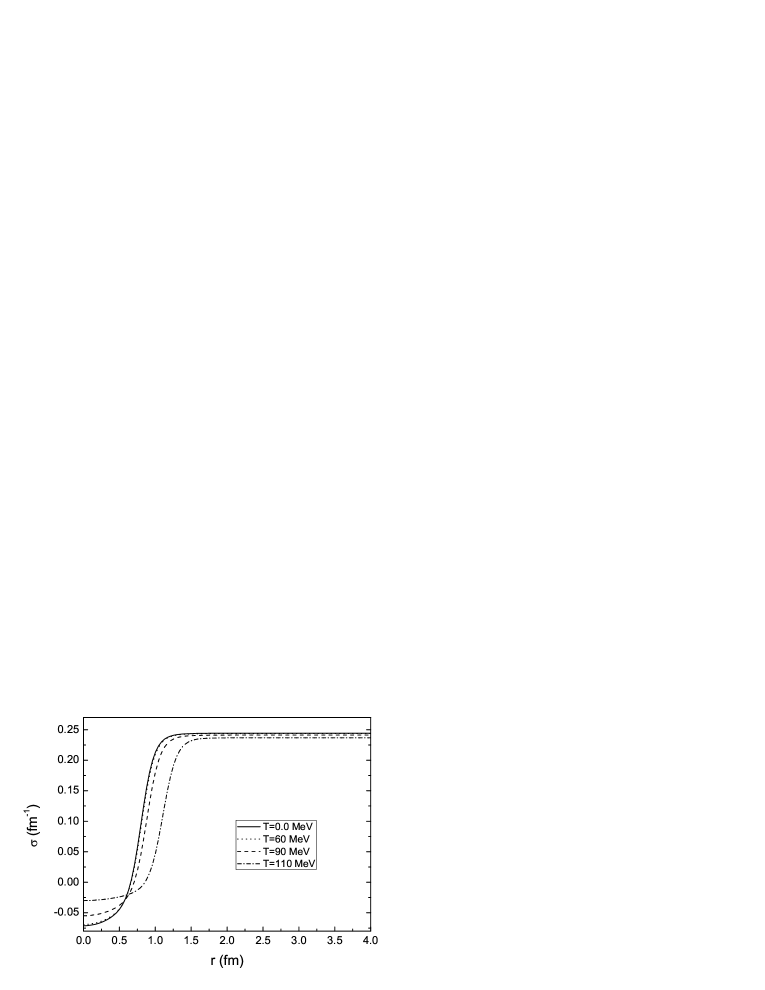
Figure 6: The soliton solutions for different temperatures when $T\leq T_{C}$.

Figure 7: Radius as functions of temperature when $T\leq T_{C}$.

The set of coupled nonlinear differential equations (17), (18) and (29) can be solved numerically with the boundary conditions Eqs.(31),(32) and (33) when the temperature is $T\leq T_{C}$. In Fig.6, we plot the soliton solutions by taking the temperatures as $T=0\mathrm{MeV},60\mathrm{MeV},90\mathrm{MeV}$ and $110\mathrm{MeV}$. From Fig.6, we can see that with the temperature increasing, $\sigma_{v}(\beta)$ is nearly constant near $\sigma_{v}$, while $\sigma(0)$ is changed dramatically. Similarly to the discussions of Ref.Zhang:2001ih , where they predicted that the radius of a stable strangelet increases as temperature increases, we can give an exact variation of radius as functions of temperature in Fig.7, which reveals that the radius of the soliton bag does increase with increasing temperature.

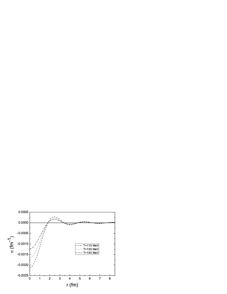
Figure 8: The solutions for the set of coupled nonlinear differential equations (17), (18) and (29) for different temperatures when $T_{C}<T$.

Figure 9: The total energy of system (soliton mass or energy)as functions of temperature when $0\leq T\leq T_{C}$, where$E_{0}$ is the soltion energy at zero temperature.

Similarly, the set of coupled nonlinear differential equations (17), (18) and (29) can be solved numerically with the boundary conditions Eqs.(31),(32) and (34) when the temperature is $T_{C}<T$. In Fig.8, we plot the solutions by taking the temperatures as $T=115\mathrm{MeV},130\mathrm{MeV}$ and $140\mathrm{MeV}$. When the temperature is higher than the critical temperature $T_{C}$, the bag constant is zero, the physical vacuum becomes unstable, and the perturbative vacuum state is stable, then the shapes of solutions are very different from that of $T\leq T_{C}$. With the increase of temperature, the soliton solutions tend to disappear. From Fig.8 we can see that, unlike the conventional soliton solutions ploted in Fig.6, here the solutions have the damping oscillation, and we can not find soliton solution anymore.

For investigating the stability of solion at different temperatures, it is necessary to calculate the total energy of the system at various temperatures by using Eq.(21), accordingly the relevant classical potential function $U(\sigma)$ should be replaced by the temperature-dependent effective potential $V(\sigma;\beta)$. In Fig.9, We plot the total energy of the system (soliton mass or energy) as functions of temperature for $0\leq T\leq T_{C}$, where$E_{0}$ is the soltion energy at zero temperature. It can be seen that the total energy of system will decrease as the temperature increases. When the temperature is around the critical temperature $T_{C}$, the total energy of the system will dramatically decrease to 74% of $E_{0}$. Since there is no soltion solution when $T>T_{C}$, the soltion mass (or energy) for $T>T_{C}$ does not exist. However, from the Fig.8 and Eq.(21), we can find that the total energy of system is almost equal to the quark field energy, this also implies that the soltion bag is melted out and has disappeared when the temperature is above the critical temperature $T_{C}$. Since there is no soliton bag when the temperature is above the critical temperature $T_{C}$, there is no mean-square charge radius for the proton for $T>T_{C}$.

As mentioned in Sect.III, $B(T)$ is defined as the difference between the vacua inside and outside the solion bag. For $T\leq T_{C}$, the vacuum inside the soliton bag is the metastable vacuum, the vacuum outside the soliton bag is the real physical vacuum. This can be seen in Fig.6. As the temperature is above the critical temperature $T_{C}$, the metastable vacuum becomes the absolute one. It can be seen from Fig.8, the behavior of $\sigma(r)$ changes dramatically when $T>T_{C}$. $\sigma(r)$ is very close to zero at any $r$. Therefore, the values of the effective potential are always close to its stable minimum at $\sigma=0$. The state at $\sigma\sim\sigma_{v}(\beta)$ can never be realized in this case. This means that the bag constant $B=0$.

Based on above analysis, there is no soliton solution and the bag constant $B(T)$ is zero for $T>T_{C}$, so there exists no more mechanism in soliton bag model to confine the quarks, and the quark is to be decofined when $T>T_{C}$.

V Summary and discussion

In this paper, we have investigated the deconfinement phase transition of the IQMDD model at finite temperature and obtained the effective potential of the IQMDD model at different temperatures. We also have gotten the function $B(T)$ and fitted the analytical formula of the bag constant. It is shown that the two minima of the potential at zero temperature will be equal at a certain temperature $T_{C}\simeq 110\mathrm{MeV}$. When the temperature $T>T_{C}$, the original perturbative vacuum state becomes stable and the original physical vacuum state becomes a metastable one. Because $\sigma(r)$ is very close to zero at any $r$ for $T>T_{C}$, the effective potential takes always its value at the absolute minimum $V(\sigma\sim 0)$. This gives $B(T)=0$ for $T>T_{C}$. As the temperature approaches another higher temperature $T\simeq 150\mathrm{MeV}$, the effective potential has a unique minimum. Our results are qualitatively similar to that obtained in conventional soltion bag model at finite temperatureGao:1992zd ; Li:1987wb ; Wang:1989ex .

In IQMDD model, the confinement of the quark requires the existence of the soliton solution, and the latter depends on the effective potential at finite temperature. In order to investigate the behavior of the soliton solution at finite temperature, we numerically solve the set of coupled nonlinear differential equations. Our results show that when $T\leq T_{C}$, there exist the stable soliton solutions in IQMDD model, but when the temperature is higher than the critical temperature $T_{C}\simeq 110\mathrm{MeV}$, there is only damping oscillation solutions and no soliton-like solution exists, and the quarks can not be confined by such solutions anymore, then the confinement of quarks are removed and the deconfined phase transition takes place. We also obtain that the radius of the soliton bag does increase when the temperature increases. At $T=T_{C}$ the soltion bag disappears.

Like the conventional soltion bag model, there are four adjustable parameters in the IQMDD model and the numerical results are also parameter-dependent. Another shortcoming of these bag models is lack of chiral symmetry. This symmetry suggests the use of a linear sigma model, which couples the quarks to pion fields as well as a scalar field. Solitons in such a model have been studied by Birse and BanerjeeBirse:1983gm Birse:1984js and Kahana, Ripka and SoniKahana:1984dx . It is of interest to extend their work to finite temperature and discuss the soliton solutions at different temperatures. Unlike the QMDTD model, where the bag constant B is put in by hand through an ansatz, we have obtained the bag constant B as a function of temperature, so our work can be used to study the effect of $s$ quarks for strange quark matter. All these works are in progress.

- (1) B. D. Serot and J. D. Walecka, Int. J. Mod. Phys. E 6, 515 (1997) and referens therein.
- (2) A.W. Tomas, Adv. in Nucl. Phys. Vol.13, 1 (New York, 1984).
- (3) E. Farhi and R. L. Jaffe, Phys. Rev. D 30, 2379 (1984); E. P. Gilson and R. L. Jaffe, Phys. Rev. Lett. 71, 332 (1993).
- (4) J. Madsen, Phys. Rev. Lett. 61 (1988) 2909; J. Madsen, Phys. Rev. D 47 (1993) 5156; J. Madsen, Phys. Rev. D 50, 3328 (1994).
- (5) C. Greiner, P. Koch and H. Stoecker, Phys. Rev. Lett. 58 (1987) 1825; C. Greiner and H. Stoecker, Phys. Rev. D 44 (1991) 3517.
- (6) G. N. Fowler, S. Raha and R. M. Weiner, Z. Phys. C 9, 271 (1981).
- (7) S. Chakrabarty, Phys. Rev. D 43 (1991) 627; S. Chakrabarty, Phys. Rev. D 48 (1993) 1409.
- (8) O. G. Benvenuto and G. Lugones, Phys. Rev. D 51 (1995) 1989; G. Lugones and O. G. Benvenuto, Phys. Rev. D 52, 1276 (1995).
- (9) G. X. Peng, H. C. Chiang and P. Z. Ning, Phys. Rev. C 62, 025801 (2000); G. X. Peng, H. C. Chiang, P. Z. Ning and B. S. Zou, Phys. Rev. C 59, 3452 (1999).
- (10) P. Wang, Phys. Rev. C 62, 015204 (2000).
- (11) Y. Zhang and R. K. Su, Phys. Rev. C 65, 035202 (2002).
- (12) Y. Zhang and R. K. Su, Phys. Rev. C 67, 015202 (2003).
- (13) Y. Zhang and R. K. Su, J. Phys. G 30, 811 (2004).
- (14) Y. Zhang and R. K. Su, Mod. Phys. Lett. A 18 (2003) 143.
- (15) Y. Zhang, R. K. Su, S. q. Ying and P. Wang, Europhys. Lett. 53, 361 (2001).
- (16) R. Friedberg and T. D. Lee, Phys. Rev. D 15, 1694 (1977); R. Friedberg and T. D. Lee, Phys. Rev. D 16, 1096 (1977); R. Friedberg and T. D. Lee, Phys. Rev. D 18, 2623 (1978).
- (17) M. C. Birse, Prog. Part. Nucl. Phys. 25, 1 (1990).
- (18) L. Wilets, World Sci. Lect. Notes Phys. 24 (1989) 1.
- (19) V. K. Gupta, A. Gupta, S. Singh and J. D. Anand, Int. J. Mod. Phys. D 12, 583 (2003).
- (20) J.Y. Shen, Y. Zhang, B. Wang and R. K. Su, Int. J. Mod. Phys. A 20, 7547 (2005).
- (21) C. Wu, W. L. Qian and R. K. Su, Phys. Rev. C 72, 035205 (2005); C. Wu, W. L. Qian and R. K. Su, Chin. Phys. Lett. 22, 1866 (2005).
- (22) D. A. Kirzhnits, JETP Lett. 15, 529 (1972) [Pisma Zh. Eksp. Teor. Fiz. 15, 745 (1972)].
- (23) D. A. Kirzhnits and A. D. Linde, Phys. Lett. B 42, 471 (1972).
- (24) S. Weinberg, Phys. Rev. D 9, 3357 (1974).
- (25) L. Dolan and R. Jackiw, Phys. Rev. D 9, 3320 (1974).
- (26) A. Das, Finite temperature field theory, Singapore, Singapore: World Scientific (1997).
- (27) T. D. Lee, “Particle Physics And Introduction To Field Theory,” Contemp. Concepts Phys. 1, (Harwood Academic, New York, 1981).
- (28) S. Gao, E. K. Wang and J. R. Li, Phys. Rev. D 46, 3211 (1992).
- (29) R. Holman, S. Hsu, T. Vachaspati and R. Watkins, Phys. Rev. D 46, 5352 (1992)
- (30) B. Carter, R. H. Brandenberger and A. C. Davis, Phys. Rev. D 65, 103520 (2002)
- (31) M. Li, M. C. Birse and L. Wilets, J. Phys. G 13 (1987) 1.
- (32) E. K. Wang, J. R. Li and L. S. Liu, Phys. Rev. D 41, 2288 (1990).
- (33) M. C. Birse and M. K. Banerjee, Phys. Lett. B 136, 284 (1984).
- (34) M. C. Birse and M. K. Banerjee, Phys. Rev. D 31, 118 (1985).
- (35) S. Kahana, G. Ripka and V. Soni, Nucl. Phys. A 415 (1984) 351.