COSMOLOGY AND NEW PHYSICS

Abstract

A comparison of the standard models in particle physics and in cosmology demonstrates that they are not compatible, though both are well established. Basics of modern cosmology are briefly reviewed. It is argued that the measurements of the main cosmological parameters are achieved through many independent physical phenomena and this minimizes possible interpretation errors. It is shown that astronomy demands new physics beyond the frameworks of the (minimal) standard model in particle physics. More revolutionary modifications of the basic principles of the theory are also discussed.

1 Introduction

Particle physics celebrates an excellent agreement of the Minimal Standard Model (MSM) with experiment, except probably for neutrino oscillations. On the other hand, cosmology also demonstrates a good agreement of astronomical observations with the standard cosmological model (SCM). So far so good, but it seems that MSM and SCM are not compatible and an explanation of the observed features of the universe is impossible without new physical phenomena. Astronomical observations have already led and will certainly lead in the near future to astonishing discoveries which may shatter cornerstones of contemporary physics and modify our understanding of basic principles.
The notion of new physics includes quite different levels of novelty:
1. New objects and/or interactions.
2. Breaking of established rules or conservation laws.
3. New principles.
This list can possibly be extended.
I. Some new physics is quite natural to expect. For example almost inevitable are:
1. New fields or/and particles: stable or quasi-stable, heavy or light.
2. Breaking of charges/quantum numbers:
a) electric, (impossible? or at least nontrivial with higher dimensions);
b) baryonic (practically certain, cosmologically discovered);
c) total leptonic (expected);
d) leptonic family(discovered in neutrino oscillations!).
Less probable:
3. Topological or non-topological solitons.
4. New types of interactions, especially new long range forces, and in particular, modified gravity at large distances.
5. Higher dimensions. It is unclear if astronomy is more sensitive to them or high energy physics. If they are small, of microscopic size then chances to “feel” them are better in high energy collisions. In the case of large higher dimensions astronomy may successfully compete with high energy physics.
II. Unnatural new physics includes
1. Breaking of Lorentz-invariance.
2. Violation of CPT.
3. Breaking of the spin-statistics relation.
4. Breaking of unitarity and quantum coherence.
5. Violation of energy conservation.
6. Violation of causality and possible existence of time-machine.
7. Breaking of least action principle, and of Hamilton and Lagrange dynamics.
III. Unexpected new physics - anything which is not in the list above and a priori will never be there.

The content of these lectures is the following. In the next section the standard cosmological model is described. In sec. 3 astronomical data characterizing the present day universe are presented. In sec. 4 the necessity of inflation is advocated and basis features of inflationary cosmology are described. Section 5 is devoted to cosmological baryogenesis and in related sec. 6 cosmological mechanisms of CP-violation are discussed. In sec. 7 the problems of vacuum and dark energies are considered. Basic features of primordial nucleosynthesis are briefly presented in sec. 8. Formation of astronomical large scale structures is discussed in sec. 9. In sec. 10 cosmological manifestations of the violation of spin-statistics theorem for neutrinos are considered. In sec. 12 we conclude.

2 Standard cosmological model

As we have already mentioned in the Introduction, the strongest demand for new physics comes from cosmology. In this connection a natural questions arise: how reliable is the standard cosmological model (SCM)? How much we can trust it? The answers to both questions are positive. In the following short few-page review we will advocate this statement. More detailed recent reviews on the basics of the modern cosmology can be found in ref. [2].

The standard cosmological model is very simple and quite robust. The theoretical setting is the following:
1. General Relativity describing gravitational interactions. It is very difficult (if possible) to modify this theory at large distances without breaking some well established fundamental physical principles.
2. Assumption (or one can say, observational fact) of homogeneous and isotropic distribution of matter in the early universe in zeroth approximation. This is supported by the smoothness of the cosmic microwave background radiation with the accuracy better than $10^{-4}$. Perturbations are treated in the first order analytically or numerical stimulated when perturbations rises up to unity.
3. Knowledge of cosmic particle content and form of their interaction. Sometimes equation of state is sufficient:

$$p_{j}=f_{j}(\rho_{j})$$ (1)

with $p_{j}$ and $\rho_{j}$ being pressure and energy densities of matter. In fact there are different forms of matter with different equations of state which is indicated by index $j$ here.

The metric describing an isotropic and homogeneous space has the form:

$$ds^{2}=dt^{2}-a^{2}(t)\,f(r)d{\bf r}^{2}$$

It is a solution of the Einstein equations with $f(r)=1+kr^{2}/4$ and $k=0$, $\pm 1$. Theory and observations agree that $k\approx 0$ with a good precision. It means that the spatial geometry of our universe is the Euclidean one.

The rate of the cosmological expansion is characterized by function $a(t)$ or more precisely by its logarithmic derivative called the Hubble parameter:

$$H={\dot{a}}/{a}$$ (2)

The Hubble parameter, is time dependent, $H\sim 1/t$, where $t$ is the universe age. The famous Hubble law is already here:

$$V=H\,l$$ (3)

where $V$ is the velocity of a distant object (which is not gravitationally binded with our Galaxy or local galactic cluster) and $l$ is the distance to it.

The equations which govern the universe expansion, i.e. time dependence of the cosmological scale factor $a(t)$ are the following:

$$\frac{\ddot{a}}{a}=-\frac{4\pi}{3m_{Pl}^{2}}(\rho+3p)$$ (4)

where $M_{Pl}=1.2\cdot 10^{19}$ GeV is the Planck mass. The Newton gravitational coupling constant is expressed through it as $G_{N}\equiv M^{-2}_{Pl}$.

Equation (4) looks as the 2nd Newton law describing the acceleration of a test body induced by matter inside radius $a$. An important fact is that not only mass (energy) creates gravitational force but also pressure. It allows for accelerated expansion, if $(\rho+3p)<0$. As is usual in general relativity, for distances $l$ larger than the inverse Hubble parameter, i.e. for $l>1/H$, the expansion becomes superluminal. These two effects are necessary for making the universe suitable for our life.

The second equation looks as the conservation of energy of a test body:

$$H^{2}\equiv\left(\frac{\dot{a}}{a}\right)^{2}=\frac{8\pi\rho}{3m_{Pl}^{2}}-\frac{k}{a^{2}}$$ (5)

If multiplied by $a^{2}/2$, the l.h.s. is the kinetic energy, while the first term in r.h.s. is negative potential energy, and the second term is just a constant.

The critical (or closure) energy density is defined as:

$$\rho_{c}=\frac{3H^{2}m_{Pl}^{2}}{8\pi}$$ (6)

It is equal to real total energy density for spatially flat universe, that is for $k=0$.

Measure of energy density of different species $j$ of any gravitating matter is expressed through the dimensionless parameter:

$$\Omega_{j}=\rho_{j}/\rho_{c}$$ (7)

Evidently if $k=0$, then $\Omega_{tot}\equiv\sum_{j}\Omega_{j}=1$.

A more adequate variable, which is often used instead of time is the red-shift, $z$:

$$z+1=a(t_{0})/a(t)$$ (8)

where $a(t_{0})$ is the value of the scale factor at the present time, so the value of red-shift today is $z=0$. For adiabatic expansion, $z$ is equal to the ratio of cosmic microwave background radiation (CMBR) temperature at some earlier time with respect to its present day value (see below).

There is one more very important equations, though not an independent one, namely, the covariant energy-momentum conservation,

$$D_{\nu}T^{\nu}_{\mu}\equiv T_{\mu;\nu}^{\nu}=0.$$ (9)

In our special homogeneous and isotropic case it looks as:

$$\dot{\rho}+3H(\rho+p)=0.$$ (10)

and follows from eqs. (4) and (5).

General relativity implies automatic conservation of $T_{\mu\nu}$ (9), due to the Einstein equations:

$$G_{\mu\nu}\equiv R_{\mu\nu}-\frac{1}{2}g_{\mu\nu}R=\frac{8\pi}{M_{Pl}^{2}}T_{\mu\nu}$$ (11)

Indeed the covariant divergence of the l.h.s. identically vanishes and so must $T_{\mu;\nu}^{\nu}$. This is a result of general covariance, i.e. invariance of physics with respect to arbitrary choice of the coordinate frame.

In recent (and not so recent) literature there are some papers where the assumption of time dependent “constants” is considered, in particular, time dependent gravitational coupling constant, $G_{N}=G_{N}(t)$ and cosmological constant $\Lambda(t)$ (about the latter see below, sec. 7). The authors of these works use there the same standard Einstein equations (11) with non-constant $M_{Pl}$. Enforcing the condition of conservation of the Einstein tensor, $G_{\mu\nu}$, and the energy-momentum tensor of matter, $T_{\mu\nu}$, the authors derive some relations between $G_{N}(t)$ and $\Lambda(t)$. However, this procedure is at least questionable. If the Einstein equations are derived as usually by functional differentiation of the total action with respect to metric, $\delta A/\delta g_{\mu\nu}=0$, then the equation must contain additional terms proportional to (second) derivatives of $G_{N}$ over coordinates. If the least action principle is rejected, then there is no known way to deduce an expression for the energy-momentum tensor of matter.

The equations of state are usually parametrized as

$$p=w\rho$$ (12)

In many practically interesting cases parameter $w$ is constant but it is not necessarily true and it may be a function of time. In this case to determine $w(t)$ one has to solve dynamical equation(s) of motion for the corresponding field(s).

Simple physical systems with $w=-1,-2/3,-1/3,0,1/3,1$ are known. They are respectively vacuum state (vacuum energy), collection of non-interacting plane domain walls and, next, straight cosmic strings, non-relativistic matter (with $p\ll\rho$), relativistic matter (with $p=\rho/3$) and the so called maximum rigid equation of state ($p=\rho$). In the last case the speed of sound is equal to the speed of light (that’s why most rigid). It can be realized by a scalar field in the course of cosmological contraction. It is strange that matter with $w=2/3$ is absent in this sequence.

One can see from eq. (4) that if $w<-1/3$ the cosmological matter anti-gravitates despite positive energy density. Correspondingly the universe expands with acceleration. It is worth to note, however, that if $\rho>0$, any matter in finite region of space has normal attractive gravity. Only infinitely large pieces of matter may anti-gravitate.

For “normal “ matter $\rho>0$ and $|\rho|>|p|$, and thus $\dot{\rho}<0$, so energy density drops down in the course of expansion, as is naturally expected. However for vacuum case the energy dominance condition, $|p|<|\rho|$, is not fulfilled $p_{vac}=-\rho_{vac}$ and the vacuum (or vacuum-like) energy density remains constant despite expansion:

$$\rho_{vac}=const$$ (13)

There might be much more strange states of matter, phantoms, with $w<-1$ [3, 4]. It such a state were realized the energy density of this kind of matter would rise in the course of expansion. As a result of this rise gravitational repulsion would become so strong that everything will be turn apart in the future, not only galaxies and stellar bodies, but even atoms and particles. This is the so-called “phantom” cosmology. In all known to me examples a constant $w<-1$ appears in some pathological models. However, it is possible that phantom state could exist only for some finite time, i.e. $w=w(t)$, and ultimately the system returns to good old state with $w\geq-1$.

It is instructive to see some simple examples of the expansion regime (we present them for the spatially flat case of $k=0$:
1. Nonrelativistic matter, $p=0$:

$$\rho\sim 1/a^{3},\,\,\,a\sim t^{2/3},\,\,\rho_{c}=m_{Pl}^{2}/6\pi t^{2}.$$ (14)

2. Relativistic matter, $p=\rho/3$:

$$\rho\sim 1/a^{4},\,\,\,a\sim t^{1/2},\,\,\rho_{c}=3m_{Pl}^{2}/32\pi t^{2}.$$ (15)

3. Vacuum(-like), $p=-\rho$:

$$\rho=const,\,\,\,a\sim e^{Ht}.$$ (16)

For normal matter the Hubble parameter decreases with time, $H\sim 1/t$, while for vacuum $H=const$. In the case of phantom cosmology $H$ would reach singularity in finite time and become infinitely large.

Presented above equations are valid of course in the ideal case of completely homogeneous universe. So they are applicable to the early universe when the matter was practically homogeneous, or to the late universe on large scales. As we mentioned above, the rise of perturbations and formation of the large scale structure (LSS) of the universe are treated in the first order approximation to the Einstein equations when the perturbations are small. Initially this is true. When perturbations became large, analytic approximations do not work and numerical simulations are applied. An analysis of LSS formation is an important part of SCM, see sec. 9. Comparison of the data with theoretical calculations allows to determine cosmological parameters and to confirm (or reject) the SCM. It is probably the weakest part of the construction but since the cosmological parameters are determined in several independent ways, the impact of theoretical ambiguities is strongly diminished.

Let us now briefly describe main epochs in the universe evolution.
1. Beginning - unknown. Maybe time did not exist before creation?
2. Inflation, i.e. period of fast (exponential) expansion which set up the frame for creation of our universe. It surely existed. Cosmological inflationary stage is practically an experimental fact.
3. Baryogenesis, generation of excess of matter over antimatter. Baryogenesis must be a dynamical process and not just a result of charge asymmetric initial conditions. In the latter case inflation would not be possible.
4. Thermally equilibrium universe, adiabatically cooled down. Some phase transitions could occur on the way, when with decreasing temperature grand unification (GUT), electroweak (EW) or QCD symmetries became broken. At such phase transitions topological solitons, e.g. monopoles, cosmic strings or even domain walls could be formed [5].
After that we come to much better known periods when all underlying physics is well known both theoretically and experimentally.
5. Neutrino decoupling. It takes place at low temperature, $T\sim 1$ MeV and is governed by the standard weak interactions.
6. Big bang nucleosynthesis (BBN). This epoch is rather spread in temperature, $T=1-0.07$ MeV and time, $t=1-200$ sec. BBN is one of the cornerstones of SCM. A good agreement of theoretical results for abundances of light elements was one of the first arguments in favor of the hot universe model.
6. Onset of the structure formation. At high temperatures the universe was dominated by relativistic matter. It is called radiation dominated (RD) stage. Structure formation in relativistic matter was inhibited and it could start only when the red-shifted as $1/a^{4}$ relativistic matter became subdominant with respect to the non-relativistic matter, which is red-shifted only as $1/a^{3}$. This epoch is called matter dominated (MD) regime. The change from RD to MD stage took place at the red-shift $z_{eq}\approx 10^{4}$ or $T\sim 1$ eV.
7. Hydrogen recombination. It takes place at $z\approx 10^{3}$ or $T\sim 3000\,{\rm K}\sim 0.2$ eV. After hydrogen recombination the cosmic plasma became practically neutral, CMBR decoupled from matter, and cosmic photons propagated freely after that. After recombination neutral hydrogen was not resisted by the radiation pressure against forming cosmic structures and baryons started infalling into already evolved seeds of structures made of dark matter.
8. Reionization, at $z=10-20$ (?) Formation of first stars.
9. Present time, $t_{U}=12-14$ Gyr.

3 Universe today

Here we will briefly present the main cosmological parameters in the contemporary universe and comment on the way of their determination.
1. Expansion rate:

$$H=100\,h\,{\rm{\rm km/sec/Mpc}}\,\,{\rm where}\,\,\,h=0.73\pm 0.05$$ (17)

The Hubble parameter is determined by direct measurement of the expansion velocity, i.e. red-shifts of some objects with presumably known luminosity (standard candles), as a function of distance and independently by the analysis of the angular fluctuations of CMBR.
2. Total energy density:

$$\rho=\rho_{c}=1.9\cdot 10^{-29}h^{2}{\rm{\frac{g}{cm^{3}}}}=10.5\,h^{2}{\rm{\frac{keV}{cm^{3}}}}\approx 10^{-47}\,{\rm{GeV^{4}}}$$ (18)

It is determined by the known value of $H$ and the fact that the universe is spatially flat, i.e. $k=0$ (see the following point, 3a).
3. Matter inventory.
a) $\Omega_{tot}=1\pm 0.1$, from the position of the first peak in the spectrum of the angular fluctuations of CMBR (figs. 1, 2) and analysis of LSS.
b) Usual baryonic matter: $\Omega_{B}=0.044\pm 0.004$ from independent measurements of the ratio of heights of the 1st and 2nd CMBR peaks, analysis of BBN, the onset of structure formation with small $\delta T/T$.
c) Total dark matter: $\Omega_{DM}\approx 0.22\pm 0.04$, from galactic rotation curves, gravitational lensing, equilibrium of hot gas in rich galactic clusters, cluster evolution, LSS.
d) The remainder: $\Omega_{DE}\approx 0.7$. This is the so called dark energy, a mysterious form of matter which anti-gravitates, i.e. induces an accelerated expansion. Its value and the fact that it is antigravitating is found from the dimming of high red-shift supernovae, LSS and the universe age.
Different pieces of data and their interpretation are independent. All above will be explained in more detail later. Error bars may be somewhat larger than those presented here.
There is a mysterious “cosmic conspiracy” between different forms of matter: the energy densities of baryons, unknown non-baryonic dark matter, and even less known dark energy have comparable values, though they could differ by many orders of magnitude. This mysterious coincidence would be even more pronounced if in addition to the usual cold dark matter there exist warm dark matter also with $\Omega_{WDM}\sim 0.1$. An understanding of this conspiracy is a long lasting challenge for theorists.

Cosmic microwave background radiation. This is the famous background of cosmic photons which was and is one of the strongest arguments in favor of the big bang cosmology. For a recent detailed review see ref. [6]; a brief digest in [7] is also helpful. The energy spectrum of CMBR has a perfect equilibrium Planck spectrum, with the temperature

$$T=2.725\pm 0.001\,{\rm{K}},$$ (19)

Correspondingly the number density of such photons in the present day universe is $n_{\gamma}=410.4\pm 0.5$ cm^-3 and their contribution into the energy density is $\Omega_{\gamma}=(4.9\pm 0.5)\cdot 10^{-5}$. The temperature of CMBR is almost isotropic over all the sky. Its angular fluctuations are very small but their significance is difficult to overestimate. They allow to observe universe at the very early stage making a snapshot of the universe at $z\approx 10^{3}$. The theoretical spectrum of the fluctuations (for some typical values of the cosmological parameters) is presented in fig. 1. The coefficients $C_{l}$ are defined as coefficients in the Legendre polynomial expansion of the correlation function of the temperature fluctuations:

$$\langle{\frac{\Delta T({\bf n})}{T}\,\frac{\Delta T({\bf n^{\prime}})}{T}}\rangle=\sum_{l}\frac{2l+1}{4\pi}\,C_{l}P_{l}(\cos\theta),$$ (20)

where ${\bf n}$ and ${\bf n^{\prime}}$ are directions of two observations and $\cos\theta={\bf n\cdot n^{\prime}}$.

The comparison of the theory with the measurements permits to to measure all basic cosmological parameters, especially if combined with other astronomical data (to lift the degeneracy). Observational data are presented in Fig. 2. (Both figures are taken from ref. [6].) There is some discrepancy between the data and theoretical expectations for low multipoles. It can be explained by the cosmic variance: since the temperature fluctuations are induced by chaotic density perturbations in the early universe, deviations from the average values for a single measurement may be large. The measured temperature fluctuations for some fixed multipole moment $l$ are averaged over all projections $m$, $-(2l+1)<m<(2l+1)$. Hence the statistical error is small for high multipoles and may be large for the low multipoles. However, small amplitudes of several low multipoles indicate to a systematic effect and may deserve a closer attention. Moreover, all low anomalously small multipoles have the same direction on the sky, the so called “evil axis”. Possibly this indicate to some, not yet understood, physical phenomena.

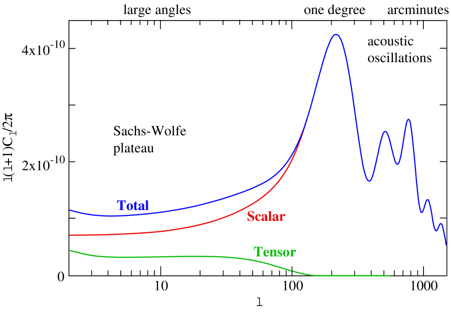
Figure 1: Theoretical angular power spectrum for adiabatic initial perturbations and typical cosmological parameters. The scalar and tensor contributions to the anisotropies are also shown.

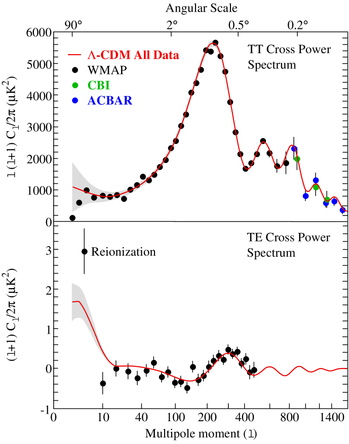
Figure 2: Temperature-temperature (TT) and temperature-polarization TE power spectra. The best fit ${\Lambda}$CDM model is also shown.

Now it is a proper place to explain, very briefly, the features of the spectrum and their relation to cosmic parameters. Any detailed discussion will demand a couple more lectures, however. There are two parts in the spectrum: more or less flat, featureless, at $l\simeq 100$ and an oscillating part for $l\geq 100$. For smaller $l$, i.e. for longer waves their length is larger than horizon at recombination. It means that the perturbations with such large wave length has not yet evolved and their amplitude is equal to the primordial one. So the part of the spectrum for $l<100$ gives direct information about spectrum of primordial perturbations. The latter is assumed to be a power law type,

$$\langle\left(\frac{\delta\rho_{k}}{\rho}\right)^{2}\rangle\sim k^{n}$$ (21)

Inflation predicts approximately this type of perturbations with $n=1$, i.e. flat or Harrison-Zeldovich spectrum. Such spectrum corresponds to featureless spectrum of gravitational potential,

$$\langle\psi_{k}^{2}\rangle\sim\frac{dk}{k}$$ (22)

without any dimensional parameter. It can be shown that for $n=1$ the power of perturbations of all wave length is the same at the moment when the corresponding wave length crosses horizon. After entering the horizon, if it happened at MD stage, the amplitudes started to rise because of gravitational instability. All long waves rise in the same manner and the spectrum is not distorted. Thus if the universe was at MD stage when long waves (corresponding to $l<100$) entered horizon, we should expect the flat curve for $(\delta T/T)^{2}$. The curves in figs. 1 and 2 are more or less of this type. However, if after MD stage the universe entered accelerated regime (we will conventionally call it vacuum dominated, or VD), the rise of perturbations becomes inhibited. The longer was the wave under horizon the stronger is the effect. Thus $(\delta T/T)^{2}$ would go down with rising $l$ and there should be a minimum between $l=0$ and $l\sim 100$. The observed minimum indeed indicates to a non-zero vacuum or dark energy and allows to measure the value the equation of state parameter, $w\approx-1$. The whole spectrum is well fitted with $n=1$ and $\Omega_{DE}\approx 0.7$.

The rise at larger $l$ is explained by acoustic oscillations at recombination. For shorter wave length and before recombination the pressure of radiation exceeds gravitational attraction. In other words, the wave length is shorter than the Jeans wave length. For such a case perturbations give rise to sound waves. The oscillations of temperature fluctuations at large $l$ is an imprint of these sounds waves on temperature of CMBR.

After recombination when the light pressure on neutral matter significantly decreased and the Jeans wave length became small, sound oscillations turned into rising density modes out of which cosmic structures were subsequently formed. However, before recombination there are no rising modes, just sound waves. At the moment of horizon crossing the amplitude of all modes were the same (for flat spectrum of perturbations). After that each mode was simply red-shifted. Shorter waves were in such red-shifted regime for a longer time and their amplitude decreased more than the amplitude of longer wave. There is one more effect of suppression of fluctuations at very short wave lengths or large $l>10^{3}$. This damping of fluctuations is induced by photon diffusion from high temperature regions to colder ones and is called diffusion or Silk damping [8]. This is more or less the picture that we see in the figures. However, on the background of the total decrease there are some peaks and minima in the spectrum. Their origin is the following. Before entering the horizon any mode consists of two parts, rising and decreasing. Evidently only rising mode survived after some time. So in this sense all the modes became coherent standing waves. If there were both modes the coherence would be destroyed and the picture with well pronounced maxima and minima would be destroyed as well. It can be shown that for adiabatic perturbations only cosine mode survives. Thus the sound wave is described by the function

$$A_{k}\cos\left[{\bf kx}\right]\,\cos\left[k\int c_{s}d\tau\right]$$ (23)

where $A_{k}$ is some slowly varying (known) function related to the spectrum of the initial perturbations and $c_{s}$ is the speed of sound, for relativistic matter it is $1/\sqrt{3}$. The amplitude of the mode with fixed $k$ is evidently

$$A_{k}\cos\left[k\int c_{s}d\tau\right]$$ (24)

The argument under the sign of the integral is just the sound horizon, which is slightly different from the cosmological horizon (by $\sqrt{3}$). Thus we see that the maximum amplitude have waves for which $kr_{s}=n\pi$ with $n=1,2,3,...$. (Note that $\tau$ is not the usual physical time but conformal time but this is simply technical issue.)

The wave with the largest amplitude is that with $n=1$. This wave just entered under horizon at the moment of recombination and did not have time to red-shift. This is the largest peak at $l\approx 200$.

The position of this peak determines 3-dimensional geometry of the universe. The physical size of the wave length corresponding to this largest peak is known. It is $r_{s}$, the sound horizon at recombination (at $T=3000$ K). The value of $l$ where the maximum is reached determines the angle under which this $r_{s}$ is observed. The angle in turn depends upon geometry of the universe. For open universe the angle would be smaller, while for closed universe it would be larger. The position at $l=200$ corresponds to flat Euclidean geometry. That’s how CMBR determines that $\Omega_{tot}=1$.

There are two more, or even maybe three more, observed peaks. The ratio of the heights of the odd and even peaks determines the amount of baryonic matter in the universe. These peaks corresponds respectively to most rarefied and compressed states. Since the oscillations proceeded in time dependent background, their amplitude depends upon the mass density of the oscillating matter. In our case it is baryonic matter, because dark matter is not coupled to photons and does not oscillate. By measurement of the ratio of the peak heights the most accurate determination of $\Omega_{b}$ was achieved.

4 Inflation

Inflation is a period of exponential (or more generally accelerated) expansion in the early universe. It was suggested [9] as a natural explanation of the very peculiar fine-tunings of the Friedman cosmology. A good introduction and reviews can be found in ref. [10]. It’s interesting that the search and discovery of inflationary solution was stimulated by a problem of overabundance of magnetic monopoles [11] which was not as important as the purely cosmological problems.

Usually an approximately exponential inflation is considered:

$$a(t)\sim\exp[Ht]$$ (25)

with ${H\approx const}$. Such a regime is easy to realize by e.g. a scalar field with slowly decreasing potential $U(\phi)$. The energy-momentum tensor of $\phi$ has the form:

$$T_{\mu\nu}=\partial_{\mu}\phi\partial_{\mu}\phi-(1/2)g_{\mu\nu}\left[\partial_{\alpha}\phi\partial^{\alpha}\phi-U(\phi)\right]$$ (26)

In slowly varying potential $\phi\approx const$, derivative terms in $T_{\mu\nu}$ can be neglected, thus $T_{\mu\nu}\sim U(\phi)g_{\mu\nu}$ and $p\approx-\rho$. This is what is necessary for exponential expansion.

There are two natural questions: why do we need such a regime and if inflation is the only known way to create the observed universe. An argument in favor of positive answers to both questions is a short list of inflationary achievements which includes at least the following:
1. Inflation solves the problem of flatness and predicts that universe today is flat with the accuracy $|\Omega-1|<10^{-4}$ (the number at the r.h.s. is the magnitude of inhomogeneities on horizon). Without inflation $\Omega$ must be fine-tuned to unity with the precision of $10^{-15}$ at BBN and $10^{-60}$ at the Planck era. With inflation it goes automatically.
2. Inflation makes all the observed universe causally connected. If not inflation, the physically connected regions on the sky would be very small, $<1^{o}$, while CMBR comes almost the same from all the sky.
3. Inflation explains the origin of expansion. This is simply because of antigravitating character of an almost constant scalar field, $3p+\rho<0$.
4. Inflation makes the universe almost homogeneous and isotropic at the present-day Hubble volume.
5. Inflation creates small inhomogeneities but at astronomically large scales, which later became seeds of large scale structure (LSS) formation. For successful realization of that the mass of the inflaton should be $m_{\phi}\sim 10^{-5}m_{Pl}$ or it should have an unnaturally weak self-coupling, $\lambda\phi^{4}$ with $\lambda\sim 10^{-14}$.

Generation of primordial density perturbations by a scalar field is possible because a scalar field, even with ${m=0}$, is not conformally invariant. Life is possible only because of breaking of scale invariance in scalar field theory.

Inflation not only solves all the above mentioned problems, which were a nightmare in the old Friedman cosmology, in an economic and elegant way but also made an important predictions of $\Omega=1$ and of adiabatic Gaussian density perturbations with flat Harrison-Zeldovich spectrum,

To solve the above mentioned problems, the inflationary period should last 60-70 Hubble times, i.e. the universe should exponentially expand by the factor $e^{60}-e^{70}$. The precise necessary value depends upon the (re)heating temperature when inflation ended. When the inflaton field $\phi$ approached zero value of its potential and $H$ became smaller than the inflaton mass, $\phi$ started to oscillate near the origin and create particles. It is almost as is described in the Bible “Let there be light” - a dark vacuum-like state exploded and created hot universe. This was a moment of Big Bang. (Re)heating temperature is model dependent and most probably is not too high, $T_{rh}<E_{GUT}\sim 10^{15}$ GeV. In this case no unwanted relics would be produced, in particular, no magnetic monopoles, which otherwise could overclose the universe [11]. The initial hot universe might be far from thermal equilibrium ( see e.g. [2, 12]) and it could facilitate baryogenesis [13].

To conclude inflation is practically an experimental fact! It is strongly confirmed by:
1. Observed ${\Omega=1}$.
2. Flat spectrum of perturbations.
3. By absence of other way to create our universe. However, be aware of danger of no-go theorems in physics, e.g. the theorem about impossibility to combine internal and space symmetries was overruled by supersymmetry. For discussion of competing with inflation cosmological models see e.g. ref. [14].

To realize inflation, a new field, inflaton, is necessary which is absent in the standard model of particle physics. Competing models also demand new physics and possibly even much more of it.

5 Baryogenesis

According to astronomical observations, the universe, at least in our neighborhood, is strongly charge asymmetric: it is populated only with particles, while antiparticles are practically absent. A small number of the observed antiprotons or positrons in cosmic rays can be explained by their secondary origin through particle collisions or maybe by the annihilation of dark matter. Any macroscopically large antimatter domains or objects (anti-stars, anti-planets or gaseous clouds of antimatter), if exist, should be quite rare. As we see in what follows, there are plenty of baryogenesis scenarios which predict either charge symmetric universe at very large scales or, even more surprising, an admixture of antimatter in our vicinity with potentially noticeable amount but still compatible with the present observational restrictions.

In connection with the observed asymmetry between matter and antimatter the first question to address is whether the observed predominance of matter over antimatter is dynamical or accidental? The former should be generated by some physical processes in the early universe starting from a rather arbitrary initial state, while the latter could be created by proper initial conditions? Such a question was sensible a quarter of century ago, but now with established inflationary cosmology, the answer may be only that any cosmological charge asymmetry could have been generated dynamically [15, 16]. The reason for that is the following. Inflation is incompatible with conserved nonzero baryonic charge density. Indeed, sufficient inflation, lasting for about $\sim$ 70 Hubble times, could proceed only if the energy density was approximately constant, see eq. (5), and $a\sim\exp(Ht)$ if $H=const$. If baryons were conserved, the energy density associated with baryonic charge (baryonic number) cannot be constant and inflation could last at most 4-5 Hubble times. Indeed any conserved charge evolves in the cosmological background as $B\sim 1/a^{3}$. Correspondingly the energy density associated with this charge cannot be constant as well and evolves as:

$$\rho_{B}\sim 1/a^{n},\,\,n=3-4$$ (27)

At RD-stage above the QCD phase transition, when quarks were massless, the baryon energy density was subdominant,

$$\rho_{B}/\rho_{tot}\approx 10^{-10}\approx const$$ (28)

Let us now travel backward in time to inflationary stage. At inflation the total energy density is supposed to be constant $\rho_{tot}=const$. This can be true if baryons are not included or negligible. The energy density of baryons rises on the way back as $\rho_{B}\sim\exp(-4Ht)$ and for $Ht>6$ the sub-dominant baryons became dominant. Thus inflation could last at most 6 Hubble times which is by far too short.

Thus initial conditions with an excess of particles over antiparticles are not compatible with inflation and dynamical generation of excess of ${B}$ over ${\bar{B}}$ is necessary. The mechanism for that was suggested by Sakharov [17]. To this end three following conditions should be fulfilled:
1. Nonconservation of baryons, theoretically natural; proved to be true in MSM and in GUT. Cosmology is an “experimental” proof: We exist ergo baryons are not conserved.
2. Breaking of C and CP, experimentally established in particle physics.
3. Deviation from thermal equilibrium. It is always true in expanding universe for massive particles or/and in the case of first order phase transitions in the primeval plasma.

There is a plenty of models of baryogenesis in the literature, for reviews see [15, 18]. There is only one number to explain, the ratio of baryonic charge density to the number density of CMBR photons:

$$\beta=\frac{n_{B}-n_{\bar{B}}}{n_{\gamma}}=\frac{n_{B}}{n_{\gamma}}|_{today}\approx 6\cdot 10^{-10}$$ (29)

Plethora of scenarios can do that but all require new physics. In principle, baryogenesis is possible in the minimal standard model of particle physics because it contains all the necessary ingredients [19]:
1. C and CP are known from experiment to be broken.
2. Baryons are not conserved because of chiral anomaly (in nonabelian theory). The charge non-conservation is achieved by some classical configuration of the Higgs and gauge boson fields, sphalerons (see however, criticism in ref. [20]).
3. Thermal equilibrium, would be strongly broken if the electroweak phase transition was first order.
So far so good. However:
1. Heavy Higgs makes 1st order p.t. improbable. Another possible source for deviation from equilibrium due to non-zero masses of ${W}$ and ${Z}$ is too weak:

$$\frac{\delta f}{f_{eq}}\sim\frac{H}{\Gamma}\sim\frac{m_{W}}{\alpha\,m_{Pl}}\sim 10^{-15}$$ (30)

2. CP violation at high T, ${T\sim T_{EW}\sim 100}$ GeV, is tiny: the amplitude of CP-breaking in MSM is proportional to the product of the mixing angles and to the mass differences of all down and all up quarks:

$$A_{-}\sim J(m_{t}^{2}-m_{u}^{2})(m_{t}^{2}-m_{c}^{2})(m_{c}^{2}-m_{u}^{2})(m_{b}^{2}-m_{s}^{2})(m_{b}^{2}-m_{d}^{2})(m_{s}^{2}-m_{d}^{2})/T^{12}$$ (31)

where

$$J=\sin\theta_{12}\,\sin\theta_{23}\sin\theta_{31}\,\sin\delta$$ (32)

is the Jarlskog determinant. At $T\geq 100$ GeV, when sphalerons were in action, $A_{-}\sim 10^{-19}$, which is too small.

It is interesting that it is necessary to have three quark families to create CP-violation in MSM through CP-odd phase in CKM matrix. Thus, if baryogenesis would be efficient in MSM, there is an “explanation” why we need 3 families. Unfortunately this is not the case and either CP breaking is different in particle physics and cosmology and we do not need three families or some modification of MSM would allow to create observable baryon asymmetry with 3 (and only 3) families.

For example one may avoid these problems and create baryon asymmetry in EW theory with 3 families if one assumes time variation of fundamental constants [21] such that

$$m_{Pl}\sim m_{EW},\,\,\,m_{q_{j}}\sim m_{EW}\,\,\,{\rm{and}}\,\,\,\delta m_{q_{j}}\sim m_{q_{j}}$$ (33)

But this is very new physics. May baryogenesis is an indication of time varying constants, TeV gravity, and large higher dimensions?!

Next very popular now scenario of creation of charge asymmetric universe is baryo-through-lepto-genesis. According to it the cosmological lepton asymmetry, $L$, could be produced by decays of heavy, $m\sim 10^{10}$ GeV, Majorana fermions. Subsequently L transformed into B by electroweak (sphaleron) processes [22] (for recent reviews see [23]). All three Sakharov’s conditions are satisfied:
1. L is naturally nonconserved.
2. Heavy particles to break thermal equilibrium are present.
3. Three CP-odd phases of order unity could be there.
The model might successfully explain the origin of the baryon asymmetry but again demands new physics: new heavy particles and new sources of CP violation are necessary.

6 CP violation in cosmology

There are three possible ways for breaking CP symmetry:
1. Standard, explicit by complex constants in Lagrangian.
2. Spontaneous [24]. This can be realized if there exists a complex scalar field with two (or several) degenerate vacuum states. The universe as a whole should be charge symmetric but locally could be asymmetric. Unfortunately domain walls between vacua with different CP-odd phases should naturally have a huge energy and thus they are cosmologically dangerous [25]. A natural way to avoid this problem is to make our domain much larger than the present day horizon. However, it make the model observationally indistinguishable from the standard one.
3. Dynamical or stochastic [26, 15, 27]. This mechanism is similar to the spontaneous one but without domain walls. It can be also realized by a complex scalar field displaced from the minimum of its potential (e.g. by quantum fluctuations during inflation), and not yet relaxed to the origin during baryogenesis. However, the field would certainly vanish to the present time and, if so, CP-violation in cosmology would have nothing in common with the observed CP-violation in particle physics.

An attractive feature of this mechanism is that a rich universe structure with isocurvature perturbations and even antimatter domains may be created. Probably it is the only chance to obtain an observational information about the mechanism of baryogenesis, because not only one number $\beta$ (29) is explained but a whole function $\beta(t,{\bf x})$ with interesting observational features is predicted. For detailed discussions see lectures [28]

7 Problem of vacuum and/or dark energy

7.1 Definition and history

As is well known the Einstein equations allow an additional term proportional to the metric tensor:

$$R_{\mu\nu}-\frac{1}{2}g_{\mu\nu}R-\Lambda\,g_{\mu\nu}=8\pi G_{N}\,T_{\mu\nu}$$ (34)

This addition was suggested by Einstein himself [29] in 1918 in an (unsuccessful) attempt to obtain stationary solutions of equations (34) in cosmological situation. The idea was that the gravitational repulsion induced by $\Lambda$ could counterbalance gravitational attraction of the ordinary matter. The fine-tuning looks unnatural and what’s more the equilibrium is evidently unstable.

This was the beginning a long and still lasting story of $\Lambda$-term. Its biography sketch looks as follows:
1. Date of birth: 1918.
2. Names: Cosmological constant, $\Lambda$-term, Vacuum Energy, or, maybe, Dark Energy.
3. Father: A. Einstein, who later, after the Hubble’s discovery of the cosmological expansion, considered his baby as “the biggest blunder of my life”. Some more quotations worth to add here. Lemaitre: “greatest discovery, deserving to make Einstein’s name famous”. Gamow: “$\lambda$ raises its nasty head again” (after indications in the 60s that quasars are accumulated near $z=2$).
4. Several times and for a long time $\Lambda$-term was assumed dead, probably erroneously. It is well alive today, but still not safe - many want to kill it.

This new term is called cosmological constant, because the coefficient $\Lambda$ must be a constant independent on space-time coordinates. Indeed, the Einstein tensor is known to be covariantly conserved:

$$D_{\mu}\left(R^{\mu}_{\nu}-\frac{1}{2}g^{\mu}_{\nu}R\right)\equiv 0$$ (35)

This property is automatic in metric theories. There is a simple analogy with electrodynamics. The Maxwell equations has the form:

$$\partial_{\mu}F^{\mu\nu}=4\pi J^{\nu}$$ (36)

Owing to antisymmetry of ${F^{\mu\nu}}$,

$$\partial_{\mu}\partial_{\nu}F^{\mu\nu}\equiv 0$$ (37)

and the current must be conserved,

$$\partial_{\mu}J^{\mu}=0.$$ (38)

On the other hand, current is conserved because of $U(1)$-invariance (gauge invariance) and the theory is self-consistent.

In the case of general relativity the situation is very similar. Automatic conservation of the Einstein tensor (35) leads to conservation of the sum:

$$D^{\mu}\left[T^{(m)}_{\mu\nu}/(8\pi m_{Pl}^{2})+\Lambda g_{\mu\nu}\right]=0$$ (39)

The energy-momentum tensor is defined as a functional derivative of the matter Lagrangian and must be conserved due to invariance of the theory with respect to arbitrary change of coordinates. Thus

$$D_{\mu}T_{\nu}^{\mu\,(m)}=0,$$ (40)

Taking into account that in metric theory the metric tensor is covariantly constant

$${D_{\mu}g^{\mu}_{\nu}\equiv 0,}$$ (41)

we come to an important conclusion that the cosmological constant must be constant:

$${{\Lambda=const}}$$ (42)

There are plenty of models in the literature with time dependent cosmological constant, $\Lambda=\Lambda(t)$. It is evident from the discussion above that such models are not innocent. One needs to introduce additional fields to satisfy the energy conservation condition or to make more serious modifications of the theory, e.g. to consider non-metric theories. The first attempt to make a time-dependent $\Lambda$, was done in 1935 by Bronshtein [30]. It was strongly criticized by Landau by the reasons presented above.

A new understanding of the nature of the cosmological constant came from quantum field theory. In its language $\Lambda$ is equivalent to vacuum energy density:

$$T_{\mu\nu}^{(vac)}=\rho_{vac}g_{\mu\nu},\,\,\,\Lambda=8\pi\rho_{vac}/m_{Pl}^{2}.$$ (43)

Quantum field theory immediately led to very serious problems. Theoretically vacuum energy should be huge, $\Lambda\approx\infty$. Mismatch between theory and upper bounds from cosmology was at the level 100-50 orders of magnitude, depending upon the type of contribution into vacuum energy. As a result the scientific establishment acquired an eclectic point of view:

$$\infty=0$$ (44)

This point of view is shared by many people even now. As Feynman said many years ago about radiative corrections in quantum electrodynamics: “Corrections are infinite but small”. However, in contrast to electrodynamics there are well defined contributions into vacuum energy which are known to be 50 or more orders of magnitude above its observed value (see below).

From 60s to the end of the Millennium vacuum energy was assumed to be identically zero. Only a few physicists treated the problem as an important one, starting from Zeldovich [31]. A non-negligible amount of scientists took a more serious attitude to $\Lambda$ only recently at the end of XX century when several independent pieces of data were accumulated which strongly indicated that empty space is not empty and it antigravitates inducing accelerated expansion. It is still unknown what induces this acceleration: vacuum with positive energy density or some other form of energy with negative pressure, $p<-\rho/3$. What makes things even more mysterious is a close proximity of $\rho_{vac}=const$ to the time varying energy density of matter $\rho_{m}\sim 1/a(t)^{3}$ exactly today. The origin of this cosmic conspiracy is necessary to understand.

7.2 Accelerated universe, data

The data at the end of 90s which led to a revolutionary change in public opinion are the following:
1.Universe age crisis. With $H\geq 70$ km/sec/Mpc the universe would be too young, $t_{U}<10$ Gyr, while stellar evolution and nuclear chronology demand $t_{U}\geq 13$ Gyr.
2. The fraction of matter density in the universe happened to be too low: $\Omega_{m}=0.3,$. The result was obtained by several independent ways: mass-to-light ratio, gravitational lensing, galactic clusters evolution (number of clusters for different red-shifts, $z=0$ and $z\sim 1$). On the other hand, inflation predicts $\Omega_{tot}=1$. Spectrum of angular fluctuations of CMBR (position of the first peak) measures $\Omega_{tot}=1\pm 0.05.$.
3. Dimming of high redshift supernovae [32] directly indicate that at $z\sim 1$ the universe started to expand with acceleration. This dimming cannot be explained by dust absorption because it was found that the effect is non-monotonic in $z$. At larger $z$ the dimming decreases, as one should expect if the effect is induced by vacuum or vacuum-like energy. Indeed, $\rho_{m}\sim 1/a^{3}$, while $\rho_{vac}=const$. Expansion goes with acceleration when $2\rho_{vac}>\rho_{m}$. For the measured present days values, $\rho_{vac}\approx 2.3\rho_{m}$, the equilibration between gravitational attraction and repulsion took place at $z\approx 0.7$ in accordance with observations.
4. LSS and CMBR well fit theory if $\Omega_{v}\approx 0.7.$ The theory of LSS formation is not free from assumptions but they are quite natural and testable. The basic inputs are: gravitational instability based on general relativity, assumption of flat spectrum of primordial fluctuations (verified by observation of low multipoles of the angular spectrum of CMBR), assumption on the type of dark matter: cold dark matter (non-interactive?), and numerical simulations when perturbations became large.

To conclude: it is established by different independent astronomical observations that vacuum or vacuum-like energy is non-vanishing. Its relative contribution into the total cosmological energy density is large in cosmological scale:

$$\Omega_{v}=0.7\,\,\,{\rm or}\,\,\,\rho_{vac}\approx 10^{-47}\,{\rm GeV}^{4}$$ (45)

and negligible on particle physics scale. All different data are consistent with

$${\Omega_{m}=0.3}\,\,\,{\rm and}\,\,\,\Omega_{tot}=1$$ (46)

7.3 Evolution of vacuum(-like) energy during cosmic history

It may be instructive to consider the role of vacuum energy during the universe life-time. At inflation $\rho_{vac}\sim 10^{100}\rho_{v}^{now}$ and was dominant. But it was not real strictly constant vacuum energy but vacuum-like energy of almost constant scalar field, inflaton. After inflaton decay to elementary particles universe was dominated by normal, presumably relativistic matter. If the reheating temperature was higher than the grand unification scale (GUT) a phase transition (p.t.) from unbroken to broken GUT state should take place. At such p.t. the change of vacuum energy was huge:

$$\Delta\rho_{vac}\approx 10^{60}\,{\rm{GeV}^{4}}$$ (47)

Whether $\rho_{vac}$ dominated or not, depended upon the order of p.t. For the second order $\rho_{vac}$ might be always subdominant, while for the first order p.t. it could dominate.

Similar picture took place at electroweak p.t. with

$$\Delta\rho_{vac}\approx 10^{8}\,{\rm GeV}^{4}$$ (48)

and at QCD p.t. with

$$\Delta\rho_{vac}\approx 10^{-2}\,{\rm{GeV}}^{4}$$ (49)

There is one important point related to QCD p.t.: the magnitudes of vacuum energies of gluon and chiral condensates, which have been formed at this p.t., are known from experiment!

After inflation till almost the present epoch $\rho_{vac}$ was always sub-dominant, with possible exception for short periods before completion of phase transitions. It started to dominate energy density only recently at $z\approx 0.3.$

7.4 Contributions to vacuum energy

According to quantum field theory all fields are represented as an infinite collection of quantum oscillators, each having energy $\omega/2$ (as in the usual quantum mechanics). The contributions to $\rho_{vac}$ from bosonic and fermionic fields have different signs because the bosonic field operators commute, while fermionic ones anti-commute. The energy density of a bosonic vacuum fluctuations is

$$\langle{\cal H}_{b}\rangle_{vac}=\int\frac{d^{3}k}{(2\pi)^{3}}\,\frac{\omega_{k}}{2}\langle a^{\dagger}_{k}a_{k}+b_{k}b^{\dagger}_{k}\rangle_{vac}=\int\frac{d^{3}k}{(2\pi)^{3}}\,\omega_{k}={\color[rgb]{1,0,0}\infty^{4}},$$

while that of fermionic one is

$$\langle{\cal H}_{f}\rangle_{vac}=\int\frac{d^{3}k}{(2\pi)^{3}}\,\frac{\omega_{k}}{2}\langle a^{\dagger}_{k}a_{k}-b_{k}b^{\dagger}_{k}\rangle_{vac}=\int\frac{d^{3}k}{(2\pi)^{3}}\,\omega_{k}=-\infty^{4},$$

where $\omega=\sqrt{k^{2}+m^{2}}$ and $m$ is the mass of the corresponding field.

One immediately sees that if there is an equal number of bosonic and fermionic fields in nature and their masses are equal (at least pairwise) then the energy of vacuum fluctuations vanishes. This was noticed by Zeldovich [31] three years before supersymmetry was discovered [33].

Indeed if the nature is supersymmetric, the number of bosonic degrees of freedom is equal to the number of fermionic ones: $N_{b}=N_{f}$ and, if SUSY is unbroken, the masses must be equal as well, $m_{b}=m_{f}$. In this case indeed $\rho_{vac}=0$. In real world, however, SUSY is broken and soft SUSY breaking, required by renormalizability of the theory, necessarily leads to

$$\rho_{vac}\sim 10^{8}\,\,{\rm GeV}^{4}\,\neq 0$$ (50)

This could be bad news for supersymmetry but the local realization of the latter which includes gravity, SUGRA [34], allows for vanishing vacuum energy even in the broken phase but at the expense of fantastic fine-tuning at the level of about $10^{-120}$, because the natural value of the vacuum energy in broken SUGRA is at the Planck scale:

$$\rho_{vac}\sim m_{Pl}^{4}\geq 10^{76}\,\,{\rm{GeV}^{4}}$$ (51)

As we have discussed in the previous subsection, in the course of cosmological expansion the cosmic plasma underwent several phase transitions at which vacuum energy changed by the amount much larger than the observed today value:

$$\Delta\rho_{vac}\gg 10^{-47}\,\,{\rm{GeV}^{4}}$$

Especially striking are QCD condensates which are known to be non-vanishing in the today’s vacuum state. QCD is well established and experimentally verified science. It leads to the conclusion that vacuum is not empty but filled with quark and gluon condensates:

$$\langle\bar{q}q\rangle\neq{0},\,\,\,\langle G_{\mu\nu}G^{\mu\nu}\rangle\neq 0$$ (52)

both having non-zero (negative and huge on cosmological scale) vacuum energy:

$$\rho_{vac}^{QCD}\approx\,-10^{45}\rho_{c}$$ (53)

The fact that this condensate must exist can be seen from the estimate of the proton mass. Proton (or neutron) consisting of three light quarks, each having mass of a few MeV, should have mass about 10-15 MeV, instead of 940 MeV. This discrepancy is solved by existence of the gluon condensate with negative energy. Inside the proton the vacuum gluon condensate is destroyed by quarks and the proton mass is:

$$m_{p}=2m_{u}+m_{d}-\rho_{vac}\,l_{p}^{3},$$ (54)

where $l_{p}\sim 1/m_{\pi}$ is the proton size and $m_{\pi}$ is the pion mass.

However outside proton gluon condensate is non-vanishing and its energy density is about $10^{45}$ larger than the cosmological energy density. The big question is who adds the necessary “donation” to make the observed $\rho_{vac}>0$ and what kind of matter is it?

7.5 Intermediate summary

We can summarize the state of art as follows:
1. Huge contributions to $\rho_{vac}$ are known but mechanism of their compensation down to (almost) zero observed value is a mystery.
2. Observed today $\rho_{vac}$ and $\rho_{m}$ differ only by factor 2, despite of very different evolution with time, $\rho_{vac}=const$ and $\rho_{m}\sim 1/t^{2}$. Why?
3. What is the nature of the antigravitating matter? Is it just vacuum energy or something different?

Mostly only problems 2 and 3 are addressed in the literature either by modification of gravity at large scales or by an introduction of a new (scalar) field (quintessence) leading to accelerated expansion.

However, most probably all three problems are strongly coupled and can be solved only together after an adjustment of $\rho_{vac}$ down to $\rho_{c}$ is understood.

7.6 Possible solutions

The list of suggestions which may in principle lead to a solution of all three problems summarized in the previous subsection is the following (possibly incomplete):
1. Subtraction constant. If dark energy is simply vacuum energy, then only one number has to be explained and theoretically it may have any value. This uncertainty reflects the unknown level of zero energy or in other words an arbitrary value of a subtraction constant. There is of course an enormous fine-tuning to fix this value just at $\rho_{c}$ but formally one cannot exclude this ugly solution. In the case that dark energy is not vacuum energy and changes with time, the subtraction constant idea is aesthetically even less appealing but still is not excluded.
2. Anthropic principle [35]. This principle excludes very large values of vacuum energy because life would not be possible in such universes. It gives a justification of a good choice of the subtraction constant. The fine-tuning in this case drops down from 100 orders to 2-3 orders of magnitude. Lacking any better suggestion, this might be a feasible solution but still not especially attractive. It reminded unsatisfactory solutions of the problems of the old Friedman cosmology before inflationary idea was proposed [9].
3. Infrared instability of massless fields (gravitons) in De Sitter space-time [36]. Massless particles are quite efficiently produced by gravitational field in exponentially expanding background. Their energy density may compensate the original vacuum energy and slow down the expansion. The mechanism looks natural and quite promising but unfortunately it seems to be inefficient.
4. Dynamical adjustment, analogous to axion solution of the problem of strong CP violation in QCD. It looks most attractive to me and because of that it is discussed below in a separate subsection.
5. Drastic modification of existing theory: higher dimensions breaking of general covariance and Lorentz invariance, a rejection of the Lagrange/Hamiltonian principle, … Maybe solution is indeed somewhere on this road but it is difficult to say today where is it exactly.

There are dozens reviews on the vacuum energy problem now. An incomplete list of recent ones are collected in ref. [37].

7.7 Dynamical adjustment

The basic idea of dynamical adjustment is extremely simple: it is assumed that there exists a new field $\Phi$ (scalar or higher spin) coupled to gravity in such a way that in De Sitter space-time a vacuum condensate of $\Phi$ is formed which compensates the original $\rho_{vac}$. This would be a manifestation of the general Le Châtelier principle on cosmological scale: the system always react in such a way as to diminish an external impact.

The dynamical adjustment was historically first [38] proposal to compensate vacuum energy down to cosmologically acceptable level. Though no satisfactory realization of the idea is found up to now, it has very attractive properties. First, vacuum energy is never compensated down to zero but only to some remainder which is generally of the order of $\rho_{c}$. In this sense dynamical adjustment idea predicted (and not postdicted) existence of dark energy with the density close to $\rho_{c}$ and thus solved mentioned above problems of compensation of the huge vacuum energy and of existence of non-compensated remnant with the proper magnitude. Byproducts of dynamical adjustment have many features of less ambitious models of modified gravity, e.g. an explicit breaking of Lorentz invariance, and a time dependent unstable background with stable fluctuations over it.

The first attempt to realize dynamical adjustment idea was based on a non-minimally coupled scalar field [38]:

$$\ddot{\phi}+3H\dot{\phi}+U^{\prime}(\phi,R)=0$$

with e.g. $U=\xi R\phi^{2}/2$. This equation has unstable, rising with time, solutions if $\xi R<0$. Asymptotically $\phi$ rises as $\phi\sim t$ and the De Sitter exponential expansion turns into Friedman power law one, but this is not due to compensation of $\rho_{vac}$ by $\rho_{\phi}$ because the energy-momentum of the latter is not proportional to the vacuum one:

$$T_{\mu\nu}(\phi)\neq Fg_{\mu\nu}$$ (55)

and the change of the regime is achieved due to weakening of the gravitational coupling:

$$G_{N}\sim 1/t^{2}$$ (56)

This is surely excluded. The models with vector [39] or tensor [3] fields were only slightly better but still did not lead to realistic cosmologies.

More recently a scalar with “crazy” coupling to gravity was considered [40, 41]:

$$A=\int d^{4}x\sqrt{g}\left[-\frac{1}{2}(R+2\Lambda)+F_{1}(R)+\frac{D_{\mu}\phi D^{\mu}\phi}{2\,R^{2}}-U(\phi,R)\right]$$ (57)

Equation of motion for $\Phi$ has the form:

$$D_{\mu}\left[D^{\mu}\phi\,\left(\frac{1}{R}\right)^{2}\right]+U^{\prime}(\phi)=0.$$ (58)

The second necessary equation is the trace of the Einstein equations. In particular case with $F_{1}=C_{1}R^{2}$ it reads:

$$-R+3\left(\frac{1}{R}\right)^{2}\left(D_{\alpha}\phi\right)^{2}-4\left[U(\phi)+\rho_{vac}\right]-6D^{2}\left[2C_{1}R-\left(\frac{1}{R}\right)^{2}\frac{\left(D_{\alpha}\phi\right)^{2}}{R}\right]=T^{\mu}_{\mu}$$ (59)

One can check that the solution of this equations tends to

$$R\sim\rho_{vac}+U(\phi)=0$$ (60)

It has some nice features (“almost realistic”), e.g. $H=1/2t$, but is unstable and easily runs away from anything resembling realistic cosmology.

A desperate attempt [41] to improve the model by introduction a non-analytic kinetic term:

$$\frac{(D\phi)^{2}}{R^{2}}\rightarrow-\frac{(D\phi)^{2}}{R\,|R|}.$$ (61)

was unsuccessful too.

More general action with scalar field [41]:

$$A=\int d^{4}x\sqrt{-g}[-{m_{Pl}^{2}}(R+2\Lambda)/16\pi+F_{1}(R)+F_{2}(\phi,R)D_{\mu}\phi D^{\mu}\phi$$

$$+F_{3}(\phi,R)D_{\mu}\phi D^{\mu}R-U(\phi,R)]$$ (62)

was not yet explored. Moreover $R_{\mu\nu}$ and $R_{\mu\nu\alpha\beta}$ can be also included.
To summarize general features of adjustment mechanism:
1. Some compensating agent must exist!
2. Quite natural to expect that $\rho_{vac}$ is not completely compensated and $\Delta\rho\sim\rho_{c}$.
3. A realistic model is needed, it can indicate what is the value of $w$: is it (-1), i.e. the non-compensated remnants of vacuum energy is also vacuum energy or $w\neq-1$ and a new strange form of energy lives in the universe?

8 Big bang nucleosynthesis

BBN or creation of light elements took place in relatively late universe, when she was from 1 to 200 sec old and temperatures were between MeV and 60-70 keV. Physics is well known at this energies. First, it is the usual low energy weak interaction leading to neutron-proton transformations:

$$n+e^{+}\leftrightarrow p+\bar{\nu}_{e},\,\,\,n+\nu_{e}\leftrightarrow p+e^{-}$$ (63)

The rate of these reactions became slow with respect to the cosmological expansion rate at $T\approx 0.7$ MeV. After that the neutron-to-proton ratio remains constant (up to the slow neutron decay) and this determines the starting value of ${n/p}$-ratio with which nucleons arrived to formation of light nuclei. The latter started and proceeded very quickly almost instantly at $T_{BBN}=60-70$ keV. The exact value of $T_{BBN}$ depends upon the baryon-to-photon ratio, $\beta$ (29). This relation allows to determine $\beta$ from BBN, especially from deuterium abundance. Though the deuterium measurements are quite dispersed, the result is in reasonable agreement with $\beta$ determined by CMBR. At $T=T_{BBN}$ all neutrons quickly formed ${{}^{4}He}$ (about 25% by mass) and a little ${{}^{2}H}$ (${3\times 10^{-5}}$ by number), ${{}^{3}He}$ (similar to ${{}^{2}H}$) and ${{}^{7}Li}$ (${10^{-9}-10^{-10}}$). The results span 9 orders of magnitude and are well confirmed by the data.

It is interesting that relatively small variation of the Fermi coupling constant would dramatically change chemical content of the universe. A slight increase of $G_{F}$ would lead to a later freezing of $(n-p)$-transformation and a smaller number of neutrons. In this case primordial universe till formation of first stars would be purely hydrogenic. In the opposite case of smaller $G_{F}$ the universe would be helium dominated. In both these extremes the properties of the first stars and their evolution would be completely different from those in our universe.

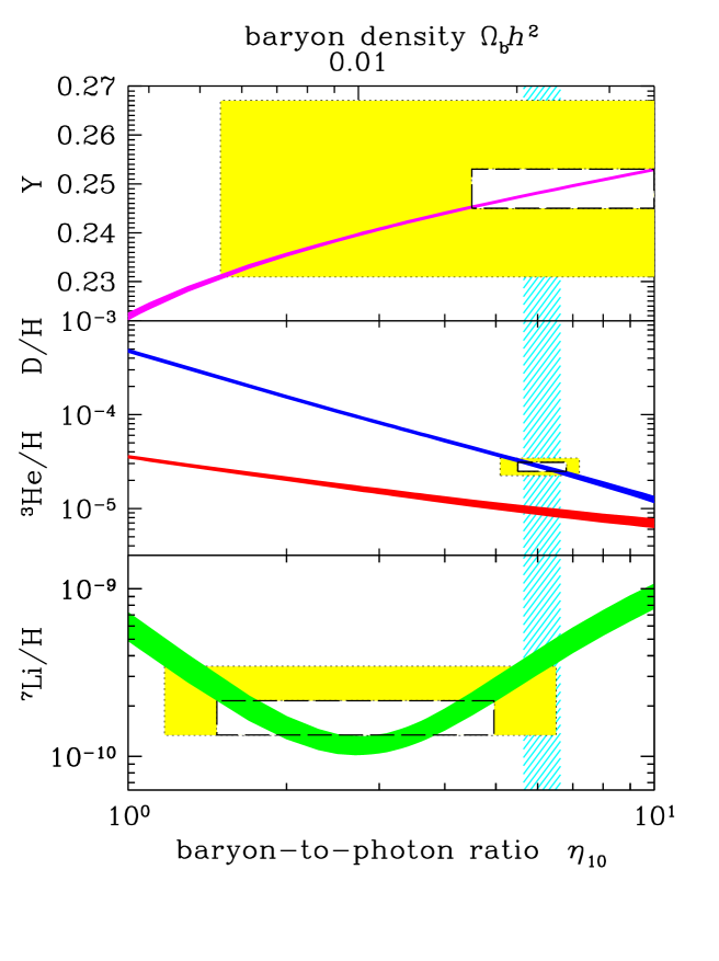
Figure 3: He⁴, D, He³ and Li⁷ predicted by the standard BBN. Boxes indicate the observed light element abundances (smaller boxes: $2\sigma$ statistical errors; larger boxes: $\pm 2\sigma$ statistical and systematic errors). The vertical band is the CMB measure of the cosmic baryon density.

Figure 4: Upper panel: the ratios of abundances of different elements in the cases of purely bosonic neutrinos with respect to the standard fermionic case as functions of the baryon number density, $\eta$. The vertically hatched (cyan) region shows the WMAP $2\sigma$ determination of $\eta$. Lower panel: the absolute abundance of ⁴He as a function of $\eta$ for the purely bosonic, Boltzmann, and fermionic neutrino distributions, corresponding to $\kappa=-1,0,+1$ respectively. The two skew hatched regions show the observation of primordial helium from ref. [42] (lower, yellow) and ref. [43] (upper, magenta), which marginally overlap at $1\sigma$.

Figure 5: The BBN values for the early universe ($\sim$ 20 minutes) baryon abundance parameter $\eta_{10}$ inferred from the adopted primordial abundances of D, ${}^{3}He$, ${}^{4}He$, and ${}^{7}Li$. Also shown is the WMAP-derived value ($\sim$ 400 kyr).

As is summarized in review [7] there is a very good agreement between theory and data on light element abundances with $\beta$ determined form CMBR, see fig. 3 taken from ref. [7] However, this picture may be too optimistic because there are some conflict between ${}^{4}He$ and ${}^{2}H$. The former corresponds to lower $\beta$. According to ref. [42] $Y=0.238\pm 0.002$, while ref. [43] finds $Y=0.2421\pm 0.0021$ ($1\sigma$, only statistical error-bars).

These results are shown in fig. 4 as the skew hatched regions, where the upper (magenta) is the results of ref. [43] and the lower (yellow) is the results of ref. [42]. In addition, different individual measurements of primordial deuterium demonstrate large dispersion and indicate to both larger and smaller $\beta$. Moreover, the trend for smaller $\beta$ demonstrates ${}^{7}Li$. For a different from [7] point of view see another review [44]. In fig. 5, taken form this work, the baryon-to-photon ratio $\eta_{10}=10^{10}\beta$ is presented as determined from different light elements abundances and is compared with that found from CMBR. There are noticeable deviations.

Most probably the discrepancy will disappear with future more accurate measurements but if it is confirmed, a strong indication to new physics will be discovered.

The data on ${}^{4}He$ and ${}^{2}H$ abundances permit to obtain an upper limit on the number of effective neutrino species, $N_{\nu}$, participating in BBN, because $N_{\nu}$ effects the cooling rate of the universe and changes the neutron-proton freezing temperature. A fair estimate is $N_{\nu}=3\pm 1$.

9 Formation of large scale structure

Formation of galaxies and their clusters is a very essential part of the modern cosmology. On one hand, it clearly demonstrates necessity of new physics and, on the other, comparison of theory with observations shows a good agreement of basic principles with the data. For a review see e.g. ref. [45].

The theoretical input is very simple: rise of the initial small density perturbations because of gravitational instability. To proceed with calculations of the structure formation one needs to know the spectrum of primordial fluctuations. Usually it is assumed power law (21). As we have already mentioned $n=1$ i.e. flat, Harrison-Zeldovich spectrum as predicted by inflation and confirmed by CMBR at large scales $l\geq 10Mpc$.

The next important step is an assumption of the properties of dark matter and dark energy. The former is normally assumed to be non-interacting cold dark matter, while dark energy is taken as the vacuum one. The corresponding cosmology is called $\Lambda$CDM. Interesting possibilities of self-interacting dark matter, e.g. mirror (for a recent review containing an impressive list of references see [46]), or warm dark matter, remain viable as well.

With these assumption one can make analytical calculations in linear regime when perturbations are small, $\delta\rho/\rho\ll 1$. To this end the standard physics, general relativity and hydrodynamics in gravitational field are used. The results are applicable to very large scales at which perturbations remain small. These scales are accessible to CMBR. The angular fluctuations of the latter are in agreement with the $\Lambda$CDM picture.

For smaller scales, $l<10$ Mpc, and larger perturbations, $\delta\rho/\rho\geq 1$, when the non-linearity of equations becomes significant one needs to make numerical simulations. The latter are of course oversimplified: the mass of individual particles are taken about $10^{6}M_{\odot}$, where $M_{\odot}=2\cdot 10^{33}$ g is the solar mass, and only gravitational interactions are taken into account. Still the description happened to be quite successful and is confirmed (but strictly speaking not proven) by the data. A large density perturbations at smaller scales (e.g. isocurvature ones) are not excluded. Their presence can invalidate the cosmological upper bounds on neutrino mass recently strengthened in numerous works [47] (possibly the list is not complete).

At this stage we can present one more argument in favor of non-baryonic dark matter. Since protons (and ${}^{4}He$-ions) strongly interact with photons, the fluctuations of baryonic matter can rise only after recombination, i.e in neutral matter. Otherwise photonic pressure prevents baryons and electrons from gravitational clumping. Density fluctuations at MD regime rise as the first power of the scale factor. Thus the density contrast in purely baryonic universe may rise at most by $10^{3}$. In the case of adiabatic fluctuations (proven by CMBR)

$$\frac{\delta\rho}{\rho}\sim\frac{\delta T}{T}<10^{-4}$$ (64)

and fluctuations could not reach unity by today in contrast to what we see. Fluctuations in non-baryonic DM do not interact with light and thus do not suffer from the pressure of CMBR. Hence fluctuations can rise at MD-stage prior recombination starting from redshift $z\sim 10^{4}$. This allows structures to be formed by the present day.

Together with the knowledge of $\Omega_{DM}=0.22$ and $\Omega_{B}=0.044$ we are forced to conclude that dark matter indeed exists and it is not the usual baryonic one. Though most of baryons in the universe are invisible their number is by far smaller than the amount of cosmological dark matter.

As for the possible forms of dark (invisible) matter, there are several (too many?) candidates. Among them are the following (but the list is far from being complete):
I. Cold dark matter (CDM): lightest supersymmetric particle (LSP), $m=(0.1-1)$ TeV; axion, ${m=10^{-5}}$ eV; mirror particles; primordial black holes.
II. Warm dark matter (WDM): sterile neutrinos ${m=0.1-1}$ keV.
III. Hot dark matter (HDM): usual neutrinos or light sterile neutrinos; they must be subdominant. Otherwise the LSS formation would be inhibited.

Thus new particles which are absent in MSM must exist. It is a striking example how astronomy predicts an existence of new elementary particles. One can make cold dark matter without new stable particles with primordial black holes with well spread mass spectrum, from a minor fraction of the solar mass up to millions of solar masses [48], but the mechanism of formation of such black holes also demands new physics.

10 Unnecessary new physics, or neutrino statistics and cosmology

This is a long standing question if statistical properties of bosons and fermions may be (slightly) different from the usual Bose-Einstein and Fermi-Dirac ones. In fact Pauli and Fermi repeatedly asked the question if spin-statistics relation could be not exact and electrons were not identical but a little bit different.

Possible violation of the exclusion principle for the usual matter, i.e. for electrons and nucleons was discussed in a number of papers at the end of the 80s [49]. Efforts to find a more general than pure Fermi-Dirac or Bose-Einstein statistics [50] were taken but no satisfactory theoretical frameworks had been found. Experimental searches of the Pauli principle violation for electrons [51] and nucleons [52] have also given negative results.

However, there is still a lot of experimental freedom to break Fermi statistics for neutrinos. In the case that spin-statistics relation is broken, while otherwise remaining in the frameworks of the traditional quantum field theory, then immediately several deep theoretical problems would emerge:
1) non-locality;
2) faster-than-light signals;
3) non-positive energy density and possibly unstable vacuum;
4) maybe breaking of unitarity;
5) broken CPT and Lorentz invariance.
To summarize there is no known self-consistent formulation of a theory with broken spin-statistics theorem. So let us postpone discussion of (non-existing) theory and consider cosmological effects of neutrinos obeying Bose or mixed statistics [53].

If neutrinos were Bose particles they could form cosmological Bose condensate:

$$f_{\nu_{b}}=\frac{1}{\exp[(E-\mu_{\nu})/T-1]}+C\delta(k),$$ (65)

and make both cold and hot dark matter. So instead of new particles obeying old physics dark matter could be created from the old known particles but with very new physics. More details can be found in ref. [53].

A deviation from Fermi statistics would be observable in BBN [54, 55]. There are two effects resulting in a change of primordial abundances:
1) the energy density of bosonic neutrinos would be 8/7 of normal fermionic $\nu$, resulting in a rise of effective neutrino species by $\Delta N_{\nu}=3/7$;
2) a larger density of $\nu_{e}$ would lead to smaller temperature of $n/p$-freezing, which is equivalent to a decrease of $N_{\nu}$.
The net result is that the effective number of neutrinos at BBN would be smaller than three: $N_{\nu}^{(eff)}=2.43$.

We assume, following ref. [55] that the equilibrium distribution for mixed statistics has the form:

$$f^{(eq)}_{\nu}=\left[\exp(E/T)+\kappa\right]^{-1},$$ (66)

where $\kappa$ interpolates between the usual Fermi statistics, $\kappa=1$, to pure Bose statistics $\kappa=-1$. Seemingly, as one can see from fig. 4 the data are noticeably better described by bosonic neutrinos. However, observational uncertainties are too large to make a definite conclusion.

If, together with spin-statistics theorem, CPT and/or unitarity is/are also broken, the usual equilibrium distributions would be distorted too and the effects can be accumulated with time and become large.

11 Some more unnecessary physics

Unfortunately time and space bounds do not allow for any detailed discussion of other unnecessary new physics as e.g. breaking of Lorenz invariance, violation of the CPT theorem, possibility of (large) higher dimensions, etc. The situation with all that is unclear and it could be that the related phenomena are not realized Though the probability of existence is low but stakes are high and new physics without any restrictions, except for experimental ones, could be very interesting. Probably cosmos will be the best place to look for these completely news effects.

A possibility of astronomical manifestations of higher dimensions, $D>4$, looks exciting. It opens practically unrestricted room for theoretical imagination. However, it may be difficult to prove their existence. We live in 4-dimensional world and most probably will not be able to penetrate other dimensions. It may be a non-trivial task to distinguish between phenomena which came to us from higher D or have a simpler (or even more complicated) explanation in $D=4$.

A very interesting effect which may arise from higher dimensions is electric charge nonconservation [56]. However, electric charge might be visibly nonconserved if photons are a little massive and in this case black holes could capture charge particles without electric hairs left outside [57]. Maybe “evil axis” could be explained by an electric charge asymmetry of the universe?

Probably in 4D world any energy nonconservation is absolutely forbidden and if it were observed, this would be an unambiguous indication that we are connected to $D>4$ space.

12 Conclusion

Cosmology unambiguously proves that there is new physics (far) beyond the minimal, and not only minimal, standard model of elementary particle world. As we have seen, inflation, which is practically an experimental fact demands a new fields or fields which had induced exponential expansion, creating “correct” universe. These field have to be very weakly coupled to the ordinary fields/particles and are absent in MSM.

Baryogenesis is impossible in MSM as well. Either heavier fields or time variation of fundamental constants are necessary. In particular the amplitude of CP-violation might be much larger in the early universe than in particle interactions at the present time.

It is proven that the bulk of matter in the universe is not the ordinary baryons. There are several good candidates for dark matter particles but it is still unknown which one is in reality. This is a primary problem for experiment and/or astronomical analysis. There is a possibility to make cosmological dark matter out of light massive neutrinos but at the expense of breaking spin-statistics theorem. The price is very high but the consequences would be exciting.

The 70%-bulk of matter in the universe, dark energy, is even more weird than ’simple” dark matter. In contrast to the ordinary matter, this dark energy induces gravitational repulsion. There can be a simple phenomenological description of cosmological acceleration by a tiny vacuum energy or by a very light scalar field (do we need that field if vacuum energy can do the job?), but only if one forgets about formidable problem of huge discrepancy, by 100-50 orders of magnitude, between the natural value of vacuum energy and the astronomically measured value. If one recalls that there are experimentally known huge contributions into vacuum energy from the quark and gluon condensates, the problem of vacuum energy compensation becomes even more striking.

One should also remember about cosmic conspiracy of the same magnitude of different forms of matter: baryonic, non-baryonic, and dark energy. Maybe a solution of this problem will indicate to some new physical effects and help to solve the vacuum energy problem?

Speaking about more revolutionary ideas of breaking unitarity, spin-statistics theorem, CPT, least action principle, etc one should be aware of Pandora box of consequences if sacred principles are destroyed. To this end a quotation from “Karamazov brothers” by Dostoevsky: “If God does not exist anything is allowed.”, may be appropriate.

References

- [1]
-
[2]
T. Padmanabhan, Lecture Course given at several places including X Special
Courses at Observatorio Nacional, Rio de Janeiro, Brazil during 26-30 Sept, 2005
astro-ph/0602117;
J. Garcia-Bellido, Proceedings of the CERN-JINR European School of High Energy Physics, San Feliu (Spain), 30 May - 12 June 2004, astro-ph/0502139;
M. Trodden, S.M. Carroll, contributions to the TASI-02 and TASI-03 summer schools, astro-ph/0401547;
I.I. Tkachev, Lectures given at the 2003 European School of High-Energy Physics, Tsakhkadzor, Armenia, 24 August – 6 September 2003, hep-ph/0405168;
J. Lesgourgues, Lecture notes for the Summer Students Programme of CERN (2002-2004), astro-ph/0409426. - [3] A.D.Dolgov, Phys.Rev. D55 (1997) 5881.
-
[4]
R.R. Caldwell, Phys. Lett. B545 (2002) 23;
R. Gannouji, D. Polarski, A. Ranquet, A.A. Starobinsky, astro-ph/0606287 (this work contains many references to earlier papers). -
[5]
A. Vilenkin, E.P.S. Shellard, Cosmic Strings and Other
Topological Defects (Cambridge University Press, Cambridge, 1994);
M.B. Hindmarsh, T.W.B. Kibble, Rep. Prog. Phys. 55 (1995) 478. M. Sakellariadou, Chapter for the book Quantum Simulations via Analogues: From Phase Transitions to Black Holes, to appear in Springer lecture notes in physics (LNP), hep-th/0602276. - [6] N. Straumann, Lectures given at the Physik-Combo, in Halle, Leipzig and Jena, 2004/5; to appear in Ann. Phys. (Leipzig), hep-ph/0505249.
- [7] S. Eidelman et al., Phys. Lett. B592 (2004) 1.
- [8] J. Silk, it Astrophys. J. 151 (1968) 459.
- [9] A. Guth, Phys. Rev. D23 (1981) 347.
-
[10]
A.D. Linde, Particle Physics and Inflationary Cosmology
(Harwood, Chur, Switzerland, 1990), hep-th/0503203;
A.D. Linde, talks at the SLAC Summer School ”Nature’s Greatest Puzzles,” at the conference Cosmo04 in Toronto, at the VI Mexican School on Gravitation, and at the XXII Texas Symposium on Relativistic Astrophysics in 2004, hep-th/0503195;
V. Mukhanov, astro-ph/0511570. -
[11]
Ya. B. Zeldovich M.Yu. Khlopov, Phys.Lett. 79 (1978) 239;
J. Preskill, Phys. Rev. Lett. 43 (1979) 1365. -
[12]
L. Kofman, Invited talk at 8th International Symposium on Particle Strings
and Cosmology (PASCOS 2001), Chapel Hill, North Carolina, 10-15 Apr 2001,
hep-ph/0107280;
R. Micha, I.I. Tkachev, Invited talk at Workshop on Strong and Electroweak Matter (SEWM 2002), Heidelberg, Germany, 2-5 Oct 2002, hep-ph/0301249. -
[13]
A.D. Dolgov, A.D. Linde, Phys. Lett. B116 (1982) 329;
E.W. Kolb, A.D. Linde, A. Riotto, Phys. Rev. Lett. 77 (1996) 4290;
E.W. Kolb,, A. Riotto, I.I. Tkachev, Phys. Lett. B423 (1998) 348;
J. Garcia-Bellido, D.Yu. Grigoriev, A. Kusenko, M.E. Shaposhnikov, Phys. Rev. D60 (1999) 123504. -
[14]
N. Turok, P.J. Steinhardt, Phys. Scripta, T117 (2005) 76;
L. Kofman, A. Linde, V.F. Mukhanov, JHEP 0210 (2002) 057. -
[15]
Dolgov A. D., Phys. Repts., 222 (1992) 309;
Dolgov A. D., Surveys in High Energy Physics, 13 (1998) 83; hep-ph/9707419. - [16] Dolgov A. D., Sazhin M. V., Zeldovich Ya. B., Basics of modern cosmology, (Gif-sur-Yvette, France, Ed. Frontieres) 1991.
- [17] Sakharov A. D., Pis’ma Zh. Eksp. Teor. Fiz., 5 (1967) 32.
-
[18]
A.G. Cohen, D.B. Kaplan, A.E. Nelson, Ann. Rev. Nucl. Sci.
43 (1993) 27;
V.A. Rubakov, M.E. Shaposhnikov, Usp. Fiz. Nauk, 166 (1996) 493; English translation: Phys. Usp. 39, (1996) 461;
A. Riotto, M. Trodden, Ann. Rev. Nucl. Part. Sci. 49 (1999) 35;
M. Dine, A. Kusenko, Rev. Mod. Phys. 76 (2004) 1. - [19] V.A. Kuzmin, V.A. Rubakov, M.E. Shaposhnikov, Phys. Lett., B155 (1985) 36.
- [20] A.D. Dolgov, Nucl. Phys. Proc. Suppl., 35 (1993) 28; also in Assergi TAUP 1993, 28.
- [21] M. Berkooz, Y. Nir, T. Volansky, Phys. Rev. Lett. 93 (2004) 051301.
- [22] M. Fukugita, T. Yanagida, Phys. Lett., bf B174 (1986) 45.
-
[23]
W. Buchmuller, P. Di Bari, M. Plumacher, New J. Phys., 6
(2004) 105;
W. Buchmuller, R.D. Peccei, T. Yanagida, hep-ph/0502169;
E.A. Paschos, Pramana, 62 (2004) 359. - [24] T.D. Lee, Phys. Rev., D8 (1973) 1226.
- [25] Ya.B. Zeldovich, I.Yu. Kobzarev, L.B. Okun, Zh. Eksp. Teor. Fiz., 67 (1974) 3 [Sov. Phys. JETP, 40 (1974) 1].
-
[26]
M.V. Chizhov, A.D. Dolgov, Nucl.Phys. B372 (1992) 521.
A.D. Dolgov, Invited talk given at Antihydrogen Workshop, Munich, Germany, 30-31 Jul 1992, hep-ph/9211241;
A.D. Dolgov, in Oak Ridge 1996, Future prospects of baryon instability search (1996) 101, hep-ph/9605280;
A.D. Dolgov, in Proceedings of 14th Rencontres de Blois: Matter - Anti-matter Asymmetry, Chateau de Blois, France, 17-22 Jun 2002, hep-ph/0211260. -
[27]
K.R.S. Balaji, T. Biswas, R.H. Brandenberger, D. London,
Phys. Lett., B595 (2004) 22;
K.R.S. Balaji, T. Biswas, R.H. Brandenberger, D. London, Phys. Rev., D72 (2005) 056005;
C.G. Branco, eConf C030603:VEN05,2003, hep-ph/0309215;
A. Kusenko, invited talk at Flavor Physics and CP Violation (FPCP), Philadelphia, Pennsylvania, 16-18 May 2002., hep-ph/0207028. - [28] A.D. Dolgov, Lectures given at International School of Physics ”Enrico Fermi”: CP Violation: From Quarks to Leptons, Varenna, Italy, 19-29 Jul 2005, hep-ph/0511213.
- [29] A. Einstein, Sitzgsber. Preuss. Acad. Wiss. 1 (1918) 142.
- [30] M. Bronstein, Physikalische Zeitschrift der Sowjetunion, 3 (1933) 73.
- [31] Ya.B. Zeldovich, Uspekhi Fiz. Nauk, 95 (1968) 209.
-
[32]
A. G. Riess et al., Supernova Search Team Collaboration,
Astron. J. 116 (1998) 1009;
S. Perlmutter et al., Supernova Cosmology Project Collaboration, Astrophys. J. 517 (1999) 565. -
[33]
Yu.A. Golfand, E.P. Likhtman, Pis’ma ZhETF, 13 (1971) 452;
D.V. Volkov, V.P. Akulov, Pis’ma ZhETF, 16 (1972) 621;
J. Wess, B. Zumino, Phys. Lett. 49 (1974) 52. -
[34]
R. Arnowitt, P. Nath, B. Zumino, Phys. Lett. 56B (1975) 81;
P. Nath, R. Arnowitt, Phys. Lett. 56B (1975) 177. -
[35]
S. Weinberg, Phys. Rev. Lett 59 (1987) 2607;
A.D. Linde, in 300 years of gravitation, ed. S.W. Hawking and W. Israel, Cambridge University Press, Cambridge, 1987, p. 621;
A. Vilenkin, Phys. Rev. Lett 74 (1995) 846;
G. Efstathiou, MNRAS, 274 (1995) L73. A. Loeb, JCAP 0605 (2006) 009 (here many references to more recent works can be found). -
[36]
N.C. Tsamis, R.P. Woodard, Phys. Lett. B301 (1993) 351;
N.C. Tsamis, R.P. Woodard, Annals of Physics, 253 (1997) 1;
A.D. Dolgov, M.B. Einhorn, V.I. Zakharov, Phys.Rev. D52 (1995) 717;
A.D. Dolgov, M.B. Einhorn, V.I. Zakharov, Acta Phys. Polon. B26 (1995) 65;
S. Habib, C. Molina-Paris, E. Mottola, Phys.Rev. D61 (2000) 024010;
R.H. Brandenberger, Plenary talk at 18th IAP Colloquium on the Nature of Dark Energy: Observational and Theoretical Results on the Accelerating Universe, Paris, France, 1-5 Jul 2002; hep-th/0210165;
R. Brandenberger, A. Mazumdar, JCAP, 0408 (2004) 015. -
[37]
V. Sahni, A. Starobinsky, Int. J. Mod. Phys. D9 (2000) 373;
P.J.E. Peebles, B. Ratra, Rev. Mod. Phys. 75 (2003) 559;
A.D. Dolgov, in “La Thuile 2004, Results and perspectives in particle physics”, p. 75 (2004) hep-ph/0405089;
S. Nobbenhuis, gr-qc/0411093;
A.D. Dolgov, Int. J. Mod. Phys. A20 (2005) 2403;
T. Padmanabhan, Phys.Repts. 380 (2005) 235;
T. Padmanabhan, Plenary talk at Albert Einstein Century International Conference at Palais de l’Unesco, Paris, France, 18-23 July, 2005; astro-ph/0603114. - [38] A.D. Dolgov in The Very Early Universe, ed. G.Gibbons, S.W.Hawking, and S.T.Tiklos (Cambridge University Press, 1982), p. 449.
- [39] A.D. Dolgov, Pisma Zh. Eksp. Teor. Fiz. 41 (1985) 280 [English translation: JETP Lett. 41 (1985) 345].
- [40] S. Mukohyama, L. Randall, Phys.Rev.Lett. 92 (2004) 211302.
- [41] A.D. Dolgov, M. Kawasaki, Phys. Atom. Nucl. 68 (2005) 828; Yad. Fiz. 68 (2005) 860.
-
[42]
B.D. Fields, K.A. Olive, Astrophys. J. 506 (1998) 177;
R.H. Cyburt, B.D. Fields, K.A. Olive, Phys. Lett. B567 (2003) 227. - [43] Y.I. Izotov, T.X. Thuan, Astrophys. J. 602 (2004) 200
- [44] G. Steigman, Int. J. Mod. Phys. E15 (2006) 1.
-
[45]
A. Loeb, lecture notes for the SAAS-Fee Winter School, April 2006,
astro-ph/0603360;
V. Springel, C.S. Frenk, S.D.M. White, Nature, 440 (2006) 1137;
N. Yoshida, it Progress of Theoretical Physics Supplement, 158 (2005) 117;
D.H. Weinberg,Science, 309 (2005) 564;
J.R. Primack, Proceedings of 6th UCLA Symposium on Sources and Detection of Dark Matter in the Universe, Marina del Rey, February 2004, astro-ph/0408359. - [46] L.B. Okun, hep-ph/0606202.
-
[47]
D.N. Spergel et al.,
Astrophys. J. Suppl. 148 (2003) 175;
S. Hannestad, JCAP, 0305 (2003) 004;
S.W. Allen, R.W. Schmidt, S.L. Bridle, Mon. Not. Roy. Astron. Soc. 346 (2003) 593;
M. Tegmark et al. [SDSS Collaboration], Phys. Rev. D69 (2004) 103501;
V. Barger, D. Marfatia, A. Tregre, Phys. Lett. B595 (2004) 55;
P. Crotty, J. Lesgourgues, S. Pastor, Phys.Rev. D69 (2004) 123007;
U. Seljak it et al [SDSS Collaboration], Phys.Rev. D71 (2005) 103515;
G.L. Fogli, E. Lisi, A. Marrone, A. Melchiorri, A. Palazzo, P. Serra J. Silk, Phys.Rev. D70 (2004) 113003;
S. Hannestad, Nucl. Phys. Proc. Suppl. 145 (2005) 313, hep-ph/0412181;
A. Goobar, S. Hannestad, E. Mortsell, H. Tu, astro-ph/0602155. - [48] A. Dolgov and J. Silk, Phys.Rev. D47 (1993) 4244.
-
[49]
A.Yu. Ignatiev, V.A. Kuzmin,Yad. Fiz. 46 (1987) 786
[Sov. J. Nucl. Phys. 46 (1987) 786];
JETP Lett. 47 (1988) 4;
L.B. Okun, Pis’ma ZhETF, 46 (1987) 420 [JETP Lett. 46 (1987) 529]; Yad. Fiz. 47 (1988) 1192;
O.W. Greenberg, R.N. Mohapatra, Phys. Rev. Lett. 59 (1987) 2507, 62 (1989) 712, Phys. Rev. D39 (1989) 2032;
A.B. Govorkov, Theor. Math. Phys. 54 (1983) 234;
A.B. Govorkov, Phys. Lett. A137 (1989) 7;
L.B. Okun, Uspekhi Fiz. Nauk, 158 (1989) 293 [Sov. Phys. Usp. 32 (1989) 543], Comments Nucl. Part. Phys. 19 (1989) 99. -
[50]
H.S. Green, Phys. Rev. 90 (1953) 270;
O.W. Greenberg, Phys. Rev. Lett. 13 (1964) 598;
O.W. Greenberg, A.M.L. Messiah, Phys. Rev. 138 (1965) B1155;
R.N. Mohapatra, Phys. Lett B242 (1990) 407;
O.W. Greenberg, A.K. Mishra, Phys. Rev. D70 (2004) 125013, math-ph/0406011. -
[51]
M. Goldhaber, G. Scharff-Goldhaber, Phys. Rev. 73 (1948) 1472;
E. Fishbach, T. Kirsten and O. Shaeffer, Phys. Rev. Lett. 20 (1968) 1012;
F. Reines, H.W. Sobel, Phys. Rev. Lett. 32 (1974) 954;
B.A. Logan, A. Ljubicic, Phys. Rev. C20 (1979) 1957;
R.D. Amado, H. Primakoff, Phys. Rev. C22 (1980) 1338;
E. Ramberg, G. Snow, Phys. Lett. B238 (1990) 438;
K. Deilamian, J. D. Gillaspy, D. Kelleher, Phys. Rev. Lett. 74 (1995) 4787;
V. M. Novikov, A. A. Pomansky, E. Nolte, JETP Lett. 51 (1990) 1;
V.M. Novikov, et al., Phys. Lett. B240 (1990) 227. -
[52]
R. Plaga, Z. Phys. A 333 (1990) 397;
A.C. Barabash, V.N. Kornoukhov, Yu.M. Tsipenyuk, V.A. Chapyzhnikov,
Pis’ma ZhETF, 68 (1998) 104
[JETP Lett. 68 (1998) 112];
The NEMO Collaboration (R. Arnold et al.) Eur. Phys. J. A6 (1999) 361;
E. Baron, R.N. Mohapatra, V.L. Teplitz, Phys. Rev. D59 (1999) 036003;
Borexino collaboration, H.O.Back, et al, hep-ph/0406252, European Physical Journal C 37 (2004) 421. -
[53]
A.D. Dolgov, A.Yu. Smirnov,
hep-ph/0501066
A.D. Dolgov, hep-ph/0504238 - [54] L. Cucurull, J.A. Grifols, R. Toldrá, Astropart.Phys. 4 (1996) 391.
- [55] A.D. Dolgov, S.H. Hansen, A.Yu. Smirnov, JCAP 0506 (2005) 004
-
[56]
S.L. Dubovsky, V.A. Rubakov, P.G. Tinyakov, JHEP, 0008 (2000) 041;
S.L. Dubovsky, V.A. Rubakov, Proceedings of Meeting on Strings and Gravity: Tying the Forces Together, Brussels, Belgium, 19-21 Oct 2001, and Proceedings of 37th Rencontre de Moriond on Electroweak Interactions and Unified Theories, Les Arcs, France, 9-16 Mar 2002, hep-th/0204205. -
[57]
A. Vilenkin, Phys. Rev. D20 (1979) 373;
B. Leaute, B. Linet, Gen. Rel. Grav. 17 (1985) 783;
A.D. Dolgov, H. Maeda, T. Torii, hep-ph/0210267.