Meson loop effect on high density chiral phase transition

Abstract

We test the stability of the mean-field solution in the Nambu–Jona-Lasinio model. For stable solutions with respect to both the $\sigma$ and $\pi$ directions, we investigate effects of the mesonic loop corrections of $1/N_{c}$, which correspond to the next-to-leading order in the $1/N_{c}$ expansion, on the high density chiral phase transition. The corrections weaken the first order phase transition and shift the critical chemical potential to a lower value. At $N_{c}=3$, however, instability of the mean field effective potential prevents us from determining the minimum of the corrected one.

At high temperature and density quantum chromodynamics (QCD) undergoes qualitative changes of great physical interest. Although many works are done, aspects of the transition region are not under full theoretical control. It is mandatory to deepen its understanding in order to understand the structure of compact stars and the history of the early universe, as well as results of ultra relativistic heavy ion experiments. With the aid of the progress in computer power, lattice simulations have become feasible for thermal system with zero or small density. In general, chiral restoration and deconfinement are expected to occur simultaneously Kogut et al. (1983). One of the most important recent findings is strong correlations in the deconfined quark gluon plasma just above the critical temperature; on the one hand it appears as the near perfect fluidity T. D. Lee (2005); Gyulassy and McLerran (2005); E. V. Shuryak (2005) and on the other hand as the mesonic correlations Asakawa and Hatsuda (2004); Ghoroku et al. (2005).

As an approach complementary to the first-principle lattice QCD simulation, we can consider effective models. In particular, they are even indispensable at high density where lattice QCD is not applicable due to the sign problem. One of them is the Nambu–Jona-Lasinio (NJL) model. Since it was proposed Nambu and Jona-Lasinio (1961a, b), although this is a model of chiral symmetry that does not possess a confinement mechanism, this model has been widely used S. P. Klevansky (1992); Hatsuda and Kunihiro (1994) in the mean field approximation, for example, for analyses of the critical end point of chiral transition on the temperature ($T$) - chemical potential ($\mu$) plane Asakawa and Yazaki (1989); Berges and Rajagopal (1999); Scavenius et al. (2000); Fujii (2003). Only a few studies that go beyond the mean field approximation were reported. Nikolov et al. E. N. Nikolov et al. (1996) extended the mean field approximation to next-to-leading order in $1/N_{c}$ which includes the meson-loop contributions. The extension preserves the symmetry property of the theory. They studied the meson loop effect in the case of $T=\mu=0$ and concluded its importance due to the light pion mass. Hüfner et al. J. Hüfner et al. (1994) formulated thermodynamics of the NJL model to order $1/N_{c}$ and Zhuang et al. Zhuang et al. (1994) presented numerical results by using the formulation. Their analyses are mainly made for thermal system in the limit of zero $\mu$. Although only a result is reported for the case that both $T$ and $\mu$ are finite, one can expect from the result that the meson loop corrections are important also for finite $\mu$.

In this Letter our attention is focused on the finite-density chiral phase transition in the limit of zero $T$. We first investigate the stability of the mean field solution and for the stable mean field solution we further evaluate the magnitude of corrections of meson loops, that is, of the next-to-leading order in the $1/N_{c}$ expansion, using the auxiliary field method of Kashiwa and Sakaguchi Kashiwa and Sakaguchi (2003) which is essentially equivalent to the formulation of Hüfner et al. J. Hüfner et al. (1994).

The Lagrangian density of the NJL model is

$$\mathcal{L}=\bar{q}(x)(i{\partial}{\mbox{\hskip 1.0pt$\not$}\hskip 8.0pt}-m_{0})q(x)+\frac{G}{2N_{c}}((\bar{q}(x)q(x))^{2}+(\bar{q}(x)i\gamma_{5}\tau_{a}q(x))^{2})\ ,$$ (1)

where $q(x)$ stands for two flavor quarks, and $N_{c}$ for the number of color degrees of freedom. $m_{0}$ is the current quark mass and $\tau_{a}$ is the Pauli matrix. $G$ is the coupling constant of a four-Fermi interactions scaled by the color number $N_{c}$ in order to use the $1/N_{c}$ expansion later. The partition function for the NJL model reads

$$Z = \int\mathcal{D}q\mathcal{D}\bar{q}\exp\Bigg{[}-\int_{\beta}d^{4}x\bigg{(}\bar{q}(x)(\partial_{\mu}\gamma^{\mu}+m_{0}-\mu\gamma_{4}-J_{\sigma}(x)-i\gamma_{5}\vec{\tau}\cdot\vec{J_{\pi}}(x))q(x)$$ (2)

$$-\frac{G}{2N_{c}}\left((\bar{q}(x)q(x))^{2}+(\bar{q}(x)i\gamma_{5}\tau_{a}q(x))^{2}\right)-\frac{N_{c}}{2G}(J_{\sigma}^{2}(x)+{\vec{J}_{\pi}}^{\,2}(x))\bigg{)}\Bigg{]}\ .$$

Here we introduced external fields $J_{\sigma}$ and $\vec{J}_{\pi}$. The last term in Eq. (2) is introduced for later convenience. $\mu$ stands for the chemical potential of quarks.

The partition function (2) has the four-Fermi interactions, accordingly we cannot carry out the Gaussian integration with respect to the quarks. Therefore, we introduce the auxiliary fields $\sigma(x)$ and $\vec{\pi}(x)$ by using of the identity

$$1=\int\mathcal{D}\sigma\exp\left[-\frac{N_{c}}{2G}\int_{\beta}d^{4}x\left(\sigma(x)+\frac{G}{N_{c}}\bar{q}(x)q(x)\right)^{2}\right]\ ,$$ (3)

and the corresponding one for $\vec{\pi}$. After integrating out quarks and shifting the auxiliary fields $(\sigma(x)-J_{\sigma}(x))\mapsto\sigma(x)$ and $(\vec{\pi}(x)-\vec{J}_{\pi}(x))\mapsto\vec{\pi}(x)$, we obtain the partition function of the auxiliary fields,

$$Z=\int\mathcal{D}\sigma\mathcal{D}\vec{\pi}\exp\left[-N_{c}I[\sigma,\vec{\pi}]\right]\ ,$$ (4)

with

$$I[\sigma,\vec{\pi}] = \int_{\beta}d^{4}x\left(\frac{1}{2G}\left(\sigma^{2}(x)+\vec{\pi}^{2}(x)\right)+\frac{1}{G}\left(\sigma(x)J_{\sigma}(x)+\vec{\pi}(x)\cdot\vec{J}_{\pi}(x)\right)\right)$$ (5)

$$-\ln\det\left(\partial_{\mu}\gamma_{\mu}+m_{0}-\mu\gamma_{4}+\sigma(x)+i\gamma_{5}\vec{\tau}\cdot\vec{\pi}(x)\right)\ .$$

The generating function for the connected Green’s function $W$ is defined as

$$Z[J_{\sigma},\vec{J}_{\pi}]\equiv\exp\left[-N_{c}W[J_{\sigma},\vec{J}_{\pi}]\right]\ .$$ (6)

The fields $\varphi_{\sigma}$ and $\vec{\varphi}_{\pi}$ are also defined as

$$\frac{\varphi_{\sigma}(x)}{G}\equiv\frac{\delta W}{\delta J_{\sigma}(x)}=\frac{\langle\sigma(x)\rangle}{G}=-\frac{1}{N_{c}}\langle\bar{q}(x)q(x)\rangle-\frac{J_{\sigma}(x)}{G}\$$ (7)

for $\varphi_{\sigma}$ and the corresponding one for $\vec{\varphi}_{\pi}$. The fields represent the vacuum expectation values of the auxiliary fields in the external fields $J_{\sigma}(x)$ and $\vec{J}_{\pi}(x)$. The effective action is defined by the Legendre transformation

$$\Gamma\left[\varphi_{\sigma},\vec{\varphi}_{\pi}\right]=W[J_{\sigma},\vec{J}_{\pi}]-\frac{1}{G}\int_{\beta}d^{4}x\left(\varphi_{\sigma}(x)J_{\sigma}(x)+\vec{\varphi}_{\pi}(x)\cdot\vec{J}_{\pi}(x)\right)\ .$$ (8)

Setting $J_{\sigma}(x)$ and $\vec{J}_{\pi}(x)$ to constants leads to the effective potential

$$\Gamma\left[\varphi_{\sigma},\vec{\varphi}_{\pi}\right]\stackrel{{\scriptstyle J_{\sigma},\vec{J}_{\pi}\mapsto\mathrm{const.}}}{{\Longrightarrow}}\beta V\mathcal{V}(\bar{\varphi}_{\sigma},\vec{\bar{\varphi}}_{\pi})\ ,$$ (9)

where note that $\varphi_{\sigma}(x)$ and $\vec{\varphi}_{\pi}(x)$ become constants $\bar{\varphi}_{\sigma}$ and $\vec{\bar{\varphi}}_{\pi}$, respectively.

In order to carry out the path integral in Eq. (4), we expand Eq. (5) around the classical solution $(\sigma_{0},\vec{\pi}_{0})$:

$$I=I_{0}+\frac{1}{2}\int_{\beta}d^{4}xd^{4}y(\sigma-\sigma_{0}\,\,\vec{\pi}-\vec{\pi}_{0})\left(\begin{array}[]{ll}I_{\sigma\sigma}^{(2)}&I_{\sigma\pi}^{(2)}\\ I_{\pi\sigma}^{(2)}&I_{\pi\sigma}^{(2)}\end{array}\right)\left(\begin{array}[]{l}\sigma-\sigma_{0}\\ \vec{\pi}-\vec{\pi}_{0}\end{array}\right)+\cdots\ ,$$ (14)

$$I_{0} = \int_{\beta}d^{4}x\left(\frac{1}{2G}(\sigma_{0}^{2}+\vec{\pi}_{0}^{2})+\frac{1}{G}(\sigma_{0}J_{\sigma}+\vec{\pi}_{0}\cdot\vec{J}_{\pi})\right)$$

$$- \ln\det(\gamma_{\mu}\partial_{\mu}+m_{0}-\mu\gamma_{4}+\sigma_{0}+i\gamma_{5}\vec{\tau}\cdot\vec{\pi}_{0})\ ,$$

$$I_{\hat{a}\hat{b}}^{(2)}=\frac{1}{G}\delta^{(4)}(x-y)\delta_{\hat{a}\hat{b}}+\mathrm{tr}[\Gamma_{\hat{a}}S(x,y:\sigma_{0},\vec{\pi}_{0})\Gamma_{\hat{b}}S(y,x:\sigma_{0},\vec{\pi}_{0})]\ ,$$ (16)

where $\Gamma_{\hat{a}}=1$ for $\hat{a}=\sigma$ and $\gamma_{5}\tau_{a}$ for $\hat{a}=\pi_{a}\,\,\,\,(a=1,2,3)$. Here the classical solutions are governed by

$$\left.\frac{\delta I}{\delta\sigma(x)}\right|_{\sigma=\sigma_{0},\vec{\pi}=\vec{\pi}_{0}}=\frac{1}{G}(\sigma_{0}(x)+J_{\sigma}(x))-\mathrm{tr}S(x,x:\sigma_{0}(x),\vec{\pi}_{0}(x))=0\ ,$$ (17)

$$\left.\frac{\delta I}{\delta\vec{\pi}(x)}\right|_{\sigma=\sigma_{0},\vec{\pi}=\vec{\pi}_{0}}=\frac{1}{G}(\vec{\pi}_{0}(x)+\vec{J}_{\pi}(x))-\mathrm{tr}\left[i\gamma_{5}\vec{\tau}S(x,x:\sigma_{0}(x),\vec{\pi}_{0}(x))\right]=0\ ,$$ (18)

$$(\gamma_{\mu}\partial_{\mu}+m_{0}-\mu\gamma_{4}+\sigma_{0}(x)+i\gamma_{5}\vec{\tau}\cdot\vec{\pi}_{0}(x))S(x,y:\sigma_{0}(x),\vec{\pi}_{0}(x))=\delta^{(4)}(x-y)\ ,$$ (19)

where $S(x,y:\sigma_{0},\vec{\pi}_{0})$ denotes the quark propagator in the external fields $J_{\sigma}(x)$. Making change of variables such that $(\sigma(x)-\sigma_{0}(x))\mapsto\sigma(x)/\sqrt{N_{c}}$ and $(\vec{\pi}(x)-\vec{\pi}_{0}(x))\mapsto\vec{\pi}(x)/\sqrt{N_{c}}$ and carrying out the Gaussian integral with respect to $\sigma(x)$ and $\vec{\pi}(x)$, we derive $W$ as

$$W[J_{\sigma},\vec{J}_{\pi}]=I_{0}+\frac{1}{2N_{c}}\mathrm{Tr}\ln{\mathbit I}^{(2)}+O\left(\frac{1}{N_{c}^{2}}\right)\ ,$$ (20)

where Tr is the trace for mesonic degrees of freedom and the spacetime coordinate. Equation (20) shows that the expansion (14) introduced above turns out to be the $1/N_{c}$ expansion. Inserting (20) into (7), we get the relation between the classical fields and the corresponding fields $\varphi_{\sigma}(x)$ and $\vec{\varphi}_{\pi}(x)$:

$$\varphi_{\sigma}(x)=\sigma_{0}(x)+\frac{G}{2N_{c}}\frac{\delta}{\delta J_{\sigma}(x)}(\mathrm{Tr}\ln{\mathbit I}^{(2)})=\sigma_{0}(x)+\frac{\sigma_{1}(x)}{N_{c}}\ ,$$ (21)

$$\vec{\varphi}_{\pi}(x)=\pi_{0}(x)+\frac{G}{2N_{c}}\frac{\delta}{\delta\vec{J}_{\pi}(x)}(\mathrm{Tr}\ln{\mathbit I}^{(2)})=\vec{\pi}_{0}(x)+\frac{\vec{\pi}_{1}(x)}{N_{c}}\ .$$ (22)

The Legendre transformation of Eq. (20) leads to

$$\mathcal{V}(\bar{\varphi}_{\sigma},\vec{\bar{\varphi}}_{\pi}) = \mathcal{V}_{0}(\bar{\varphi}_{\sigma},\vec{\bar{\varphi}}_{\pi})+\mathcal{V}_{1}(\bar{\varphi}_{\sigma},\vec{\bar{\varphi}}_{\pi})\ ,$$ (23)

$$\mathcal{V}_{0}(\bar{\varphi}_{\sigma},\vec{\bar{\varphi}}_{\pi}) = \frac{1}{2G}(\bar{\varphi}_{\sigma}^{2}+\vec{\bar{\varphi}}_{\pi}^{2})-\frac{1}{\beta V}\ln\det(\gamma_{\mu}\partial_{\mu}+m_{0}-\mu\gamma_{4}+\bar{\varphi}_{\sigma}+i\gamma_{5}\vec{\tau}\cdot\vec{\bar{\varphi}}_{\pi})\ ,$$ (24)

$$\mathcal{V}_{1}(\bar{\varphi}_{\sigma},\vec{\bar{\varphi}}_{\pi}) = \frac{1}{2N_{c}\beta V}\mathrm{Tr}\ln{\mathbit I}^{(2)}(\bar{\varphi}_{\sigma},\vec{\bar{\varphi}}_{\pi})+O\left(\frac{1}{N_{c}^{2}}\right)\ .$$ (25)

The leading term $\mathcal{V}_{0}$ corresponds to the contribution of the mean field approximation and the the next-to-leading contribution $\mathcal{V}_{1}$ to the contribution of meson loops of $1/N_{c}$ order.

Actual calculation of the effective potential (23) is done in the momentum representation. The mean field part $\mathcal{V}_{0}$ is represented as

$$\mathcal{V}_{0} = \frac{1}{2G}((M-m_{0})^{2}+\vec{\bar{\varphi}}_{\pi}^{2})$$ (26)

$$- 2N_{f}\int\frac{d^{3}p}{(2\pi)^{3}}\left[E_{{\mathbit p}}+\frac{1}{\beta}\ln(1+\mathrm{e}^{-\beta(E_{{\mathbit p}}+\mu)})+\frac{1}{\beta}\ln(1+\mathrm{e}^{-\beta(E_{{\mathbit p}}-\mu)})\right]\ ,$$

where $E_{{\mathbit p}}=({\mathbit p}^{2}+M^{2}+\vec{\bar{\varphi}}_{\pi}^{2})^{1/2}$ and $M=m_{0}+\bar{\varphi}_{\sigma}$. The mesonic loop correction part $\mathcal{V}_{1}$ becomes

$$\mathcal{V}_{1}=\frac{1}{2N_{c}}[A_{\sigma}(T,\mu)+3A_{\pi}(T,\mu)]\ ,$$ (27)

$$A_{\hat{a}}=\frac{1}{\beta}\sum_{n=-\infty}^{\infty}\int\frac{d^{3}p}{(2\pi)^{3}}\ln\left(\frac{1}{G}-I_{1}(i\omega_{n}^{b},{\mathbit p})+((i\omega_{n}^{b})^{2}-{\mathbit p}^{2}-\varepsilon_{\hat{a}}^{2})I_{2}(i\omega_{n}^{b},{\mathbit p})\right)\ ,$$ (28)

where

$$I_{1}(i\omega_{n}^{b},{\mathbit p}) = 2N_{f}\bigg{[}\int\frac{d^{3}q}{(2\pi)^{3}}\frac{1}{2E_{{\mathbit q}}}\left[1-f(E_{{\mathbit q}}+\mu)-f(E_{{\mathbit q}}-\mu)\right]$$ (29)

$$+\int\frac{d^{3}q}{(2\pi)^{3}}\frac{1}{2E_{{\mathbit p}+{\mathbit q}}}\left[1-f(E_{{\mathbit p}+{\mathbit q}}+\mu)-f(E_{{\mathbit p}+{\mathbit q}}-\mu)\right]\bigg{]}\ ,$$

$$\mathrm{Re}I_{2}(i\omega_{n}^{b},{\mathbit p})=-\frac{N_{f}}{4}\int\frac{d^{3}q}{(2\pi)^{3}}\frac{1}{E_{{\mathbit p}+{\mathbit q}}E_{{\mathbit q}}}$$

$$\times\Bigg{[}\frac{E_{{\mathbit p}+{\mathbit q}}-E_{{\mathbit q}}}{{\omega_{n}^{b}}^{2}+(E_{{\mathbit p}+{\mathbit q}}-E_{{\mathbit q}})^{2}}(f(E_{{\mathbit p}+{\mathbit q}}+\mu)+f(E_{{\mathbit p}+{\mathbit q}}-\mu)-f(E_{{\mathbit q}}+\mu)-f(E_{{\mathbit q}}-\mu))$$

$$+\frac{E_{{\mathbit p}+{\mathbit q}}+E_{{\mathbit q}}}{{\omega_{n}^{b}}^{2}+(E_{{\mathbit p}+{\mathbit q}}+E_{{\mathbit q}})^{2}}(2-f(E_{{\mathbit p}+{\mathbit q}}+\mu)-f(E_{{\mathbit p}+{\mathbit q}}-\mu)-f(E_{{\mathbit q}}+\mu)-f(E_{{\mathbit q}}-\mu))\Bigg{]}\ ,$$ (30)

$$\mathrm{Im}I_{2}(i\omega_{n}^{b},{\mathbit p}) = N_{f}\int\frac{d^{3}q}{(2\pi)^{3}}\frac{\omega_{n}^{b}}{({\omega_{n}^{b}}^{2}+E_{{\mathbit p}+{\mathbit q}}^{2}+E_{{\mathbit q}}^{2})^{2}-4E_{{\mathbit p}+{\mathbit q}}^{2}E_{{\mathbit q}}^{2}}$$ (31)

$$\times(f(E_{{\mathbit q}}+\mu)-f(E_{{\mathbit q}}-\mu)-f(E_{{\mathbit p}+{\mathbit q}}+\mu)+f(E_{{\mathbit p}+{\mathbit q}}-\mu))\ ,$$

with $\omega_{n}^{b}=2\pi n/\beta$ and $f(E)\equiv 1/(\mathrm{e}^{\beta E}+1)$. In the limit of zero temperature, these equations are reduced to simpler forms:

$$\mathcal{V}_{0} \stackrel{{\scriptstyle T\to 0}}{{\longrightarrow}} \frac{1}{2G}((M-m_{0})^{2}+\vec{\bar{\varphi}}_{\pi}^{2})-2N_{f}\int\frac{d^{3}p}{(2\pi)^{3}}\left[\mu+(E_{{\mathbit p}}-\mu)\theta(E_{{\mathbit p}}-\mu)\right]\ ,$$ (32)

$$A_{\hat{a}} \stackrel{{\scriptstyle T\to 0}}{{\longrightarrow}} \int\frac{d\omega}{2\pi}\int\frac{d^{3}p}{(2\pi)^{3}}\ln\left(\frac{1}{G}-I_{1}(i\omega,{\mathbit p})+((i\omega)^{2}-{\mathbit p}^{2}-\varepsilon_{\hat{a}}^{2})I_{2}(i\omega,{\mathbit p})\right)\ ,$$ (33)

$$I_{1}(i\omega,{\mathbit p}) = 2N_{f}\bigg{[}\int\frac{d^{3}q}{(2\pi)^{3}}\frac{1}{2E_{{\mathbit q}}}\theta(E_{{\mathbit q}}-\mu)+\int\frac{d^{3}q}{(2\pi)^{3}}\frac{1}{2E_{{\mathbit p}+{\mathbit q}}}\theta(E_{{\mathbit p}+{\mathbit q}}-\mu)\bigg{]}\ ,$$ (34)

$$\mathrm{Re}I_{2}(i\omega,{\mathbit p}) = -\frac{N_{f}}{4}\int\frac{d^{3}q}{(2\pi)^{3}}\frac{1}{E_{{\mathbit p}+{\mathbit q}}E_{{\mathbit q}}}$$ (35)

$$\times\Bigg{[}\frac{E_{{\mathbit p}+{\mathbit q}}-E_{{\mathbit q}}}{{\omega}^{2}+(E_{{\mathbit p}+{\mathbit q}}-E_{{\mathbit q}})^{2}}(\theta(E_{{\mathbit q}}-\mu)-\theta(E_{{\mathbit p}+{\mathbit q}}-\mu))$$

$$+\frac{E_{{\mathbit p}+{\mathbit q}}+E_{{\mathbit q}}}{{\omega}^{2}+(E_{{\mathbit p}+{\mathbit q}}+E_{{\mathbit q}})^{2}}(\theta(E_{{\mathbit q}}-\mu)+\theta(E_{{\mathbit p}+{\mathbit q}}-\mu))\bigg{]}\ ,$$

$$\mathrm{Im}I_{2}(i\omega,{\mathbit p})$$ (36)

$$= N_{f}\int\frac{d^{3}q}{(2\pi)^{3}}\frac{\omega}{({\omega}^{2}+E_{{\mathbit p}+{\mathbit q}}^{2}+E_{{\mathbit q}}^{2})^{2}-4E_{{\mathbit p}+{\mathbit q}}^{2}E_{{\mathbit q}}^{2}}(\theta(E_{{\mathbit q}}-\mu)-\theta(E_{{\mathbit p}+{\mathbit q}}-\mu))\ ,$$

where note that $\omega$ becomes a continuous valuable.

In the present analysis, we adopt the parameter set of Hatsuda and Kunihiro Hatsuda and Kunihiro (1987) which are determined so as to reproduce $F_{\pi}=93$ MeV and $m_{\pi}=138$ MeV at $T=\mu=0$; the resultant values are $m_{0}=5.5$ MeV, the four-Fermi coupling constant $G=32.976$ GeV^-2 and the ultra-violet divergence cutoff $\Lambda=631$ MeV.

Figure 1 represents the effective potential at $\mu=330,340,348$ and $500$ MeV. When $\mu=330$ MeV, there appears a minimum around $M=340$ MeV at the mean field level. The stability of the mean field solution can be investigated by the curvature of $\mathcal{V}_{0}$ in the $\bar{\varphi}_{\sigma}$ and $\bar{\varphi}_{\pi}$ directions. In the region denoted by “$\sigma$ unstable”, the curvature is negative and then unstable in the $\bar{\varphi}_{\sigma}$ direction. Similarly, in the region denoted by “$\pi$ unstable”, the curvature is negative in the $\bar{\varphi}_{\pi}$ direction. Fortunately, the minimum around $M=340$ MeV is out of the unstable regions. This property is held for other values of $\mu$; three examples are shown in other panels of Fig. 1. As another interesting point, any $\pi$ unstable region does not appear for $\mu>330$ MeV. Thus, the mean field solution at the minimum point is stable at any $\mu$ for the case of the present parameter set.

The meson loop corrections in the unstable regions do not make sense, since mesons considered there are tachyonic. Actually, the Gaussian integral in Eq.(4) breaks down for tachyonic mesons. Note that dashed curves in the unstable regions are just a guide of eyes. In the $N_{c}=3$ case, we can not see where is a minimum, since it is somewhere in the unstable regions. So we take a somewhat larger $N_{c}$, or 20, in which a minimum is still out of the unstable regions even after the inclusion of the correction. We then look into the effect of the next-to-leading order correction by comparing the mean field solution (the $N_{c}\rightarrow\infty$ case) and the finite $N_{c}$ ($=20$) case.

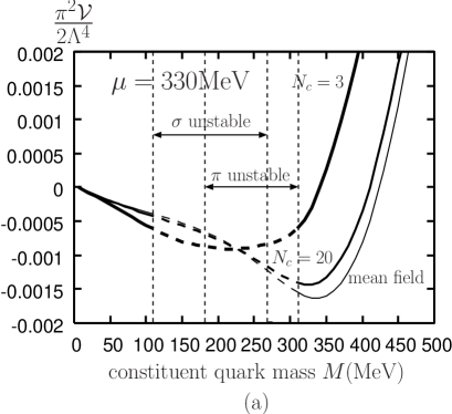
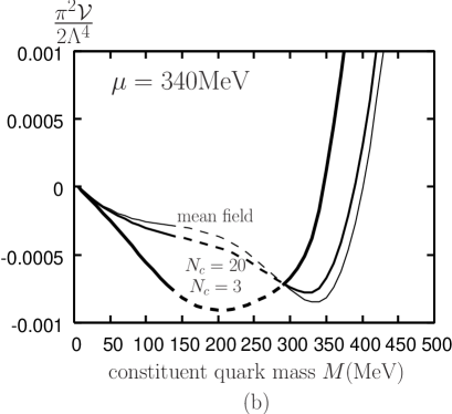
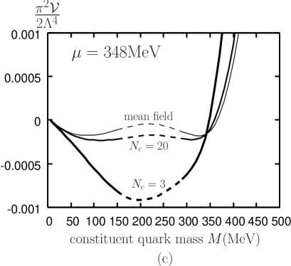
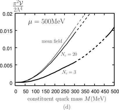
Fig. 1: Non-dimensionalized effective potential as a function of the constituent quark mass. Cases of four different chemical potentials are presented. Thickness of curves decreases as the number of color increases as $3\rightarrow 20\rightarrow\infty$. Dashed curves indicate regions unstable with respect to the $\sigma$ and/or $\pi$ directions. For $\mu=330$ MeV, regions unstable in the $\sigma$ ($\pi$) direction are denoted by “$\sigma$ unstable” (“$\pi$ unstable”). For $\mu>330$ MeV, all regions denoted by dashed curves are unstable only in the $\sigma$ direction.

First we discuss the result of the mean field approximation. Studies in the mean field approximation level have already been done in Refs. Berges and Rajagopal (1999); Asakawa and Yazaki (1989); Scavenius et al. (2000); Fujii (2003). At $\mu=$ 340 MeV (Fig. 1(b)) the minimum is still located around $M=$ 340 MeV; this means that chiral symmetry is broken. At $\mu=$ 348 MeV (Fig. 1(c)) two minima degenerate; in other words this is the first order phase transition point. At higher $\mu$ (Fig. 1(d)) chiral symmetry is restored to some extent. Here a comment is in order. In this case $M$ at the minimum is still around 50 MeV, and it decreases gradually as $\mu$ increases; in other words we see a crossover to the restored phase. This situation was seen also in Refs. Asakawa and Yazaki (1989); Scavenius et al. (2000) although not discussed.

Now we consider the next-to-leading order correction due to a finite $N_{c}$. In the case of $N_{c}=20$ the results are similar to the mean field case but the correction weakens the transition, in other words makes the jump in $M$ small and shifts the critical $\mu$ to a lower value. These are clearly shown in Fig. 2.

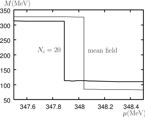
Fig. 2: The value of the constituent quark mass at which the effective potential becomes minimum as a function of the chemical potential. The mean field and the $N_{c}=20$ cases are presented.

To summarize, we have studied semi-quantitatively the effects of the mesonic, i.e., the next-to-leading order in the $1/N_{c}$ expansion, correction in the Nambu–Jona-Lasinio model on the high density chiral phase transition based on the auxiliary field method. The finite $N_{c}$ correction weakens the first order phase transition and shifts the critical chemical potential to a lower value. At $N_{c}=3$, however, we can not see the minimum because of the instability of the mean field effective potential to the direction of the $\sigma$ and/or $\pi$ classical fields. For the mean field calculation, we have pointed out explicitly that chiral symmetry is not completely restored immediately at the first order transition; after the first order transition the constituent quark mass decreases gradually — this may be called the two step restoration.

We still have a lot to do: First of all we have to redetermine the parameter set, the four-Fermi coupling constant $G$ and the ultra-violet cutoff $\Lambda$ in the next-to-leading order. Next we have to study the phase diagram at finite $T$ and $\mu$ to find the location of the critical end point. Further, studies of the three flavor model and the color superconductivity phase are to be done.

References

Kogut et al. (1983)
J. Kogut,
M. Stone,
H. W. Wyld,
W. R. Gibbs,
J. Shigemitsu,
S. H. Shenker, and
D. K. Sinclair, Phys. Rev. Lett. 50, 393
(1983).
T. D. Lee (2005)
T. D. Lee, Nucl. Phys.
A750, 1 (2005).
Gyulassy and McLerran (2005)
M. Gyulassy and
L. McLerran,
Nucl. Phys. A750,
30 (2005).
E. V. Shuryak (2005)
E. V. Shuryak, Nucl. Phys. A750, 64
(2005).
Asakawa and Hatsuda (2004)
M. Asakawa and
T. Hatsuda,
Phys. Rev. Lett. 92,
012001 (2004).
Ghoroku et al. (2005)
K. Ghoroku,
T. Sakaguchi,
N. Uekusa, and
M. Yahiro,
Phys. Rev. D 71,
106002 (2005).
Nambu and Jona-Lasinio (1961a)
Y. Nambu and
G. Jona-Lasinio,
Phys. Rev. 122,
345 (1961a).
Nambu and Jona-Lasinio (1961b)
Y. Nambu and
G. Jona-Lasinio,
Phys. Rev. 124,
246 (1961b).
S. P. Klevansky (1992)
S. P. Klevansky, Rev. Mod. Phys. 64, 649
(1992).
Hatsuda and Kunihiro (1994)
T. Hatsuda and
T. Kunihiro,
Phys. Rep. 247,
221 (1994).
Asakawa and Yazaki (1989)
M. Asakawa and
K. Yazaki,
Nucl. Phys. A504,
668 (1989).
Berges and Rajagopal (1999)
J. Berges and
K. Rajagopal,
Nucl. Phys. B538,
215 (1999).
Scavenius et al. (2000)
O. Scavenius,
Á. Mócsy,
I. N. Mishustin, and
D. H. Rischke, Phys. Rev. C 64, 045202
(2000).
Fujii (2003)
H. Fujii,
Phys. Rev. D 67,
094018 (2003).
E. N. Nikolov et al. (1996)
E. N. Nikolov,
W. Broniowski,
C. V. Christov,
G. Ripka, and
K. Goeke,
Nucl. Phys. A608,
411 (1996).
J. Hüfner et al. (1994)
J. Hüfner,
S. P. Klevansky, and
P. Zhuang,
Ann. Phys. 234,
225 (1994).
Zhuang et al. (1994)
P. Zhuang,
J. Hüfner, and
S. P. Klevansky, Nucl. Phys. A576, 525
(1994).
Kashiwa and Sakaguchi (2003)
T. Kashiwa and
T. Sakaguchi,
Phys. Rev. D 68,
065002 (2003).
Hatsuda and Kunihiro (1987)
T. Hatsuda and
T. Kunihiro,
KEK preprint 159 (1987).