Abstract

We report on a calculation of the ‘mixed’ strong and (purely) weak corrections through the order $\alpha_{\mathrm{S}}^{2}\alpha_{\mathrm{W}}$ to parton-parton processes in all possible channels at hadron colliders entering the single jet inclusive cross section. At both Tevatron and LHC, such effects are always negligible (below permille level) in the total integrated cross section whilst they become sizable in differential rates. Specifically, if such corrections are defined with respect to the full leading-order result of ${\cal O}(\alpha_{\mathrm{S}}^{2}+\alpha_{\mathrm{S}}\alpha_{\mathrm{EW}}+\alpha_{\mathrm{EW}}^{2})$, we find that, at the FNAL accelerator, they can reach the $-5\%$ benchmark in the jet transverse energy (at the kinematical limit of the machine, rendering their detection quite difficult). At the CERN collider, in the same observable, they exceed the $-10\%$ level already at 1 TeV and can reach $-40\%$ at 4 TeV, kinematic regions where such corrections will be comfortably observable for standard luminosity. In addition, such corrections are somewhat sensitive to the factorisation/renormalisation scale choice.

Keywords: Hadron Colliders, Electroweak physics, Higher-order calculations.

1 Introduction

As the centre-of-mass (CM) energy of present and future hadron colliders increases well beyond the Electro-Weak (EW) scale, of ${\cal O}$(100 GeV), such as at the Tevatron at FNAL ($\sqrt{s}_{p\bar{p}}=1.96$ TeV) and the Large Hadron Collider (LHC) at CERN ($\sqrt{s}_{pp}=14$ TeV), it is clear that the impact of higher order EW corrections, particularly of the purely Weak (W) component, will become more and more important phenomenologically, with respect to similar Quantum Chromo-Dynamics (QCD) effects [1]. The reason is twofold. On the one hand, the strong coupling ‘constant’, $\alpha_{\mathrm{S}}$, decreases with increasing energy faster than the EW one, $\alpha_{\mathrm{W}}\equiv\alpha_{\mathrm{EM}}/\sin^{2}\theta_{W}$ (with $\alpha_{\mathrm{EM}}$ the Electro-Magnetic (EM) coupling constant and $\theta_{W}$ the weak angle). On the other hand, the purely weak part of higher order EW effects produces leading corrections of the type $\alpha_{\rm{W}}\log^{2}({\mu^{2}}/M_{W}^{2})$, wherein $\mu$ represents some typical energy scale affecting the hard process in a given observable, e.g., the partonic CM energy $\sqrt{\hat{s}}$. For large enough $\mu$ values, such W effects may be competitive not only with Next-to-Next-to-Leading-Order (NNLO) (as $\alpha_{\rm{W}}\approx\alpha_{\rm{S}}^{2}$) but also with NLO QCD corrections (e.g., for ${\mu}=0.5$ TeV, $\log^{2}({\mu^{2}}/M_{W}^{2})\approx 10$). (Clearly, in actual calculations, combinatorial effects, colour/flavour factors as well as subleading terms will have to appropriately be accounted for.) These ‘double logs’ are of Sudakov origin and are due to a lack of cancellation between virtual and real $W$-emission in higher order contributions. This is in turn a consequence of the violation of the Bloch-Nordsieck theorem in non-Abelian theories [2]. (See Refs. [3, 4] for comprehensive reviews.)

The problem is in principle present also in QCD. In practice, however, it has no observable consequences, because of the final averaging of the colour degrees of freedom of partons, forced by confinement into colourless hadrons. This does not occur in the EW case, where the initial state generally has a non-Abelian charge, such as in proton-(anti)proton collisions. Besides, these logarithmic corrections are finite (unlike in QCD), since $M_{W}$ provides a physical cut-off for $W$-emission. Hence, for typical experimental resolutions, softly and collinearly emitted weak bosons need not be included in the production cross section and one can restrict oneself to the calculation of weak effects originating from virtual corrections only [5]. By doing so, similar logarithmic effects, $\sim\alpha_{\rm{W}}\log^{2}({\mu^{2}}/M_{Z}^{2})$, are also generated by virtual corrections due to $Z$-bosons. Finally, in some instances, all these purely weak contributions can be isolated in a gauge-invariant manner from EM effects which therefore may not be included in the calculation (as it is the case here). (Notice that QED corrections, just like QCD ones, are not subject to Sudakov enhancement.)

Furthermore, physics Beyond the Standard Model (BSM), if due to right-handed weak currents [6], contact interactions or compositeness [7] or new massive gauge bosons $W^{\prime},Z^{\prime}$ [8, 9] may well manifest itself in deviations from the SM in jet quantities (which eventually emerge as observables of parton-parton collisions after hadronisation: see [10]–[17] for definitions and reviews of standard algorithms for hadronisation and jet evolution), such as jet transverse energy $E_{T}$ or di-jet invariant masses $M_{jj}$. The lower bounds on typical $W^{\prime},Z^{\prime}$ masses from direct searches at Tevatron are model dependent but are typically around $500-600\,\mbox{GeV}$ [18], whilst the LHC can access such massive gauge bosons with masses up to $4-4.5\,\mbox{TeV}$ [19]. Whilst typical compositeness limits from Tevatron are very mild, compared to the EW scale, the LHC can probe (with planned high luminosity) jet transverse energies of about 4 TeV or so, where the possible existence of quark substructures could be manifest. Moreover, a tenfold increase in luminosity, as the one currently been discussed for the so-called Super-LHC (SLHC) option, would give access to jets of up to $E_{T}\approx 5$ TeV [20].

The plan of the paper is as follows. In the next Section we describe the subprocesses that we have computed in terms of topologies of Feynman diagrams. Sect. 3 illustrates the computational techniques adopted. Sects. 4 and 5 present our results for Tevatron and LHC, respectively. Sect. 6 summarises our work and draws the main conclusions. Finally, in the appendix, we describe in detail the helicity amplitude formalism adopted here, also giving some specific formulae for (some of) the topologies discussed in Sect. 2.

2 The subprocesses

In view of what explained in the previous section, it becomes of crucial importance to assess the quantitative relevance of one-loop weak effects entering via ${\cal O}(\alpha_{\mathrm{S}}^{2}\alpha_{\mathrm{W}})$ the fifteen possible $2\to 2$ partonic subprocesses responsible for jet production in hadronic collisions, namely:

$$gg \to q\bar{q}$$ (1)

$$q\bar{q} \to gg$$ (2)

$$qg \to qg$$ (3)

$$\bar{q}g \to \bar{q}g$$ (4)

$$qq \to qq$$ (5)

$$\bar{q}\bar{q} \to \bar{q}\bar{q}$$ (6)

$$qQ \to qQ~{}({\rm{same~{}generation}})$$ (7)

$$\bar{q}\bar{Q} \to \bar{q}\bar{Q}~{}({\rm{same~{}generation}})$$ (8)

$$qQ \to qQ~{}({\rm{different~{}generation}})$$ (9)

$$\bar{q}\bar{Q} \to \bar{q}\bar{Q}~{}({\rm{different~{}generation}})$$ (10)

$$q\bar{q} \to q\bar{q}$$ (11)

$$q\bar{q} \to Q\bar{Q}~{}({\rm{same~{}generation}})$$ (12)

$$q\bar{q} \to Q\bar{Q}~{}({\rm{different~{}generation}})$$ (13)

$$q\bar{Q} \to q\bar{Q}~{}({\rm{same~{}generation}})$$ (14)

$$q\bar{Q} \to q\bar{Q}~{}({\rm{different~{}generation}}),$$ (15)

with $q$ and $Q$ referring to quarks of different flavours, limited to $u$-, $d$-, $s$-, $c$- and $b$-type, all taken as massless. Whilst the first four processes (with external gluons) were already computed in Ref. [21], the eleven four-quark processes were tackled in Refs. [22, 23] (see also [24]). Furthermore, these four-quark processes can have Infra-Red (IR) divergences, both soft and collinear, so that gluon bremsstrahlung effects ought to be evaluated to obtain a finite cross section at the considered order. In addition, for completeness, we have also included the non-divergent $2\to 3$ subprocesses

$$qg \to qq\bar{q}$$ (16)

$$\bar{q}g \to \bar{q}\bar{q}q$$ (17)

$$qg \to qQ\bar{Q}~{}({\rm{same~{}generation}})$$ (18)

$$\bar{q}g \to \bar{q}\bar{Q}Q~{}({\rm{same~{}generation}}).$$ (19)

(See Refs. [25, 26] for tree-level $\alpha_{\mathrm{S}}\alpha_{\mathrm{EW}}$ and $\alpha_{\mathrm{EW}}^{2}$ interference effects.) As intimated in the Introduction, we will instead ignore altogether the contributions of tree-level $\alpha_{\mathrm{S}}^{2}\alpha_{\mathrm{W}}$ terms involving the radiation of $W$- and $Z$-bosons. This presumes that the adopted jet definition efficiently vetoes against those gauge bosons decaying inside the jets and the detector coverage minimises the loss of all their decays. We will return to this matter later on in the paper.

Before proceeding to describe the calculation we have performed, we list the ‘topologies’ involved (i.e., Feynman graphs without reference to specific couplings or internal masses) and briefly discuss their most salient phenomenological aspects.

• Processes 1 ($gg\rightarrow q\bar{q}$) and 2 ($q\bar{q}\rightarrow gg$) (Figs. 1, 2):
  The two processes with a gluon pair in the initial or final state do not exist through ${\cal O}(\alpha_{\rm S}\alpha_{\rm W})$ (as we need at least four quark-gluon vertices) thus the one-loop weak corrections to $\alpha_{\rm S}^{2}$ correspond to the leading order weak calculation. The $\alpha_{\rm S}^{2}\alpha_{\rm W}$ calculation is IR finite and therefore we do not include gluon bremsstrahlung diagrams.

• Processes 3 ($qg\rightarrow qg$) and 4 ($\bar{q}g\rightarrow\bar{q}g$) (Figs. 3, 4):
  Comments made for the previous two processes also hold in this case.

• Processes 5 ($qq\rightarrow qq$) and 6 ($\bar{q}\bar{q}\rightarrow\bar{q}\bar{q}$) (Fig. 5):
  The full calculation for these processes will have a contribution from order $\alpha_{\rm S}\alpha_{\rm W}$ and requires gluon bremsstrahlung diagrams, meaning that a subtraction procedure will have to be enforced in order to cancel the IR divergences between the real and virtual parts of the calculation (see later on for further details on the techniques adopted to achieve such a cancellation). Naturally, $W$-exchange is here confined to self-energy and vertex corrections.

• Processes 7 ($qQ\rightarrow qQ$ (same generation)) and 8 ($\bar{q}\bar{Q}\rightarrow\bar{q}\bar{Q}$ (same generation)) (Fig. 7):
  Hereafter, notice that we assume a flavour diagonal Cabibbo-Kobayashi-Maskawa (CKM) mixing matrix for quarks. The approximation is justified by the unitarity of such a matrix, the small value of the Cabibbo angle and by the fact that contributions from top quarks are negligible in comparison to those from light quarks. Besides, this approximation considerably simplifies the calculation.

• Processes 9 ($qQ\rightarrow qQ$ (different generation)) and 10 ($\bar{q}\bar{Q}\rightarrow\bar{q}\bar{Q}$ (different generation)) (Fig. 8):
  The diagrams that contribute to process 9(10) are a subset of those that contribute to process 7(8). As a consequences of the assumption made for the CKM matrix, we ignore here the interaction where a $W$-emission/absorption changes a quark generation index and as such the $W$-mediated graphs connecting the two fermion lines that contribute to processes 7 and 8 are ignored in 9 and 10, respectively. For the same reason, there is no tree-level $\alpha_{\rm S}\alpha_{\rm W}$ contribution here.

• Process 11 ($q\bar{q}\rightarrow q\bar{q}$) (Figs. 9, 10, 11):
  This is possibly the most involved process of all, in terms of number of different topologies, though $W$-corrections are limited to the case of self-energies and triangles.

• Process 12 ($q\bar{q}\rightarrow Q\bar{Q}$ (same generation)) (Fig. 12):
  The topologies are here a subset of those involved in the previous process, upon replacing appropriately $Z$- with $W$-exchange between the two fermion lines.

• Process 13 ($q\bar{q}\rightarrow Q\bar{Q}$ (different generation)) (Fig. 13):
  The graphs involved here are a subset of the previous process, as $W$-exchange between the two fermion lines is not present. In addition, unlike the previous case, there is no allowed interference that contributes at order $\alpha_{\rm S}\alpha_{\rm W}$ to this process, due to the vanishing of the colour factors.

• Process 14 ($q\bar{Q}\rightarrow q\bar{Q}$ (same generation)) (Fig. 14):
  $W$-exchange between the two fermion lines here only occurs in annihilation diagrams, unlike all previous cases, where it takes place in scattering graphs only.

• Process 15 ($q\bar{Q}\rightarrow q\bar{Q}$ (different generation)) (Fig. 15):
  The graphs involved here are a subset of the previous process, as $W$-exchange between the two fermion lines is not present. As in process (13) there is no allowed interference that contributes at order $\alpha_{\rm S}\alpha_{\rm W}$ to this process, as all possibilities have vanishing colour factors.

• Processes 16 ($qg\rightarrow qq\bar{q}$) and 17 ($\bar{q}g\rightarrow\bar{q}\bar{q}q$) (Fig. 16):
  These processes are IR finite as there are no possible bremsstrahlung diagrams we can write down at $\alpha_{\rm S}^{2}\alpha_{\rm W}$ order.

• Processes 18 ($qg\rightarrow qQ\bar{Q}$ (same generation)) and 19 ($\bar{q}g\rightarrow\bar{q}\bar{Q}Q$ (same generation)) (Fig. 16):
  The same comments as in the previous case are valid here in the context of IR finiteness. Note also that there are no processes analogous to processes 18 and 19 with quarks of different generations as there are no contributing interferences at the required order.

3 The calculation

Given the large number of diagrams involved in the computation, it is of paramount importance to perform careful checks. In this respect, we should mention that our expressions have been calculated independently by at least two of us using FORM [27] and that some results have also been reproduced by another program based on FeynCalc [28]. (See the Appendix for more details on the procedure adopted for the tensor reduction and amplitude calculation.) We also find reasonable agreement with Ref. [29] in the Sudakov limit, i.e., for large invariant masses and transverse momenta of the final state, provided that the final state particles are fairly central.

As already mentioned, IR divergences occur when the virtual or real (bremsstrahlung) gluon is either soft or collinear with the emitting parton and these have been dealt with by using the formalism of Ref. [30], whereby corresponding dipole terms are subtracted from the bremsstrahlung contributions in order to render the phase space integral free of IR divergences. The integration over the gluon phase space of these dipole terms was performed analytically in $d$-dimensions, yielding pole terms which cancelled explicitly against the pole terms of the virtual graphs. There remains a divergence from the initial state collinear configuration, which is absorbed into the scale dependence of the PDFs and must be matched to the scale at which these PDFs are extracted. Through the order at which we are working, it is sufficient to take the LO evolution of the PDFs (and thus the one-loop running of $\alpha_{\rm{S}}$).

The self-energy and vertex correction graphs contain Ultra-Violet (UV) divergences that have been subtracted here by using the ‘modified’ Dimensional Reduction (${\overline{\mathrm{DR}}}$) scheme at the scale $\mu=M_{Z}$. The use of ${\overline{\mathrm{DR}}}$, as opposed to the more usual ‘modified’ Minimal Subtraction (${\overline{\mathrm{MS}}}$) scheme, is forced upon us by the fact that the $W$- and $Z$-bosons contain axial couplings which cannot be consistently treated in ordinary dimensional regularisation. Thus the values taken for the running $\alpha_{\rm S}$ refer to the ${\overline{\mathrm{DR}}}$ scheme whereas the EM coupling, $\alpha_{\mathrm{EM}}$, has been taken to be $1/128$ at the above subtraction point. The one exception to this renormalisation procedure has been the case of the self-energy insertions on external fermion lines, which have been subtracted on mass-shell, so that the external fermion fields create or destroy particle states with the correct normalisation.

The top quark entering the loops in reactions with external $b$’s has been assumed to have mass $m_{t}=175$ GeV and width $\Gamma_{t}=1.55$ GeV. The $Z$-mass used was $M_{Z}=91.19$ GeV and was related to the $W$-mass, $M_{W}$, via the SM formula $M_{W}=M_{Z}\cos\theta_{W}$, where $\sin^{2}\theta_{W}=0.232$. (Corresponding widths were $\Gamma_{Z}=2.5$ GeV and $\Gamma_{W}=2.08$ GeV.) Also notice that Higgs contributions are not included here, as required by all quarks being massless. For the strong coupling constant, $\alpha_{\rm S}$, we have used the one- or two-loop expression with $\Lambda^{(n_{\rm f}=4)}_{\overline{\mathrm{MS}}}$ chosen to match the value required by the LO and NLO Parton Distribution Functions (PDFs) used. The latter were CTEQ6L1 (our default) plus CTEQ6L at LO and CTEQ6M at NLO [31], respectively.

The fully differential cross sections for processes (1)–(19) are obtained numerically in FORTRAN as follows

$$d\sigma=(2\pi)^{4}\delta^{4}\left(\sum p_{i}-\sum p_{f}\right){{1}\over{2\hat{s}}}\left(\prod_{f}{{d^{3}{\bf p}_{f}}\over{(2\pi)^{3}2E_{f}}}\right)|{\cal A}|^{2}f_{1}^{p}(x_{1})f_{2}^{p(\bar{p})}(x_{2})dx_{1}dx_{2},$$ (20)

wherein $p_{i(f)}=(E_{i(f)},{\bf p}_{i(f)})$ are the initial(final) particle momenta, $|{\cal A}|^{2}$ the amplitude squared averaged(summed) over initial(final) colours and helicities, $x_{i}$ the usual Bjorken momentum fractions and $f_{i}^{p(\bar{p})}$ the proton(antiproton) PDFs. (For convenience we will refer to $f_{1}^{p}(x_{1})f_{2}^{p(\bar{p})}(x_{2})dx_{1}dx_{2}$ – assuming a summation over all possible quark and gluon combinations – as the parton luminosity.) Finally, the integrations over the two- or three-body phase spaces and the $x$’s have been performed using VEGAS [32]. (A simple change of kinematic variables yields the $E_{T}$ dependence of the cross section discussed below.)

4 Tevatron phenomenology

A detailed discussion for the case of Tevatron, geared to comparisons against existing data from Run 1 and 2, can be found in Ref. [23]. This is mainly a discussion on the impact of ${\cal O}(\alpha_{\mathrm{S}}^{2}\alpha_{\mathrm{W}})$ one-loop virtual corrections on high $E_{T}$ jet samples, where an excess was initially found by CDF (but not D0) during Run 1 [35], with respect to the NLO QCD predictions [36]–[39]. It was eventually pointed out that a modification of the gluon PDFs at medium/large Bjorken $x$ [40] can reconcile theory and data, even within current systematics: see, e.g., [41]. In fact, notice that with the most recent PDFs (e.g., CTEQ6.1M [31]), the preliminary Run 2 data also seem to be consistent with NLO QCD, see [42] for CDF, albeit barely. The question as to whether ${\cal O}(\alpha_{\mathrm{S}}^{2}\alpha_{\mathrm{W}})$ effects may be required in a future comparison between theory and data comparisons (or in the parameterisation of the PDFs) is still open [43] and such effects are presently being implemented in the fastNLO package [44].

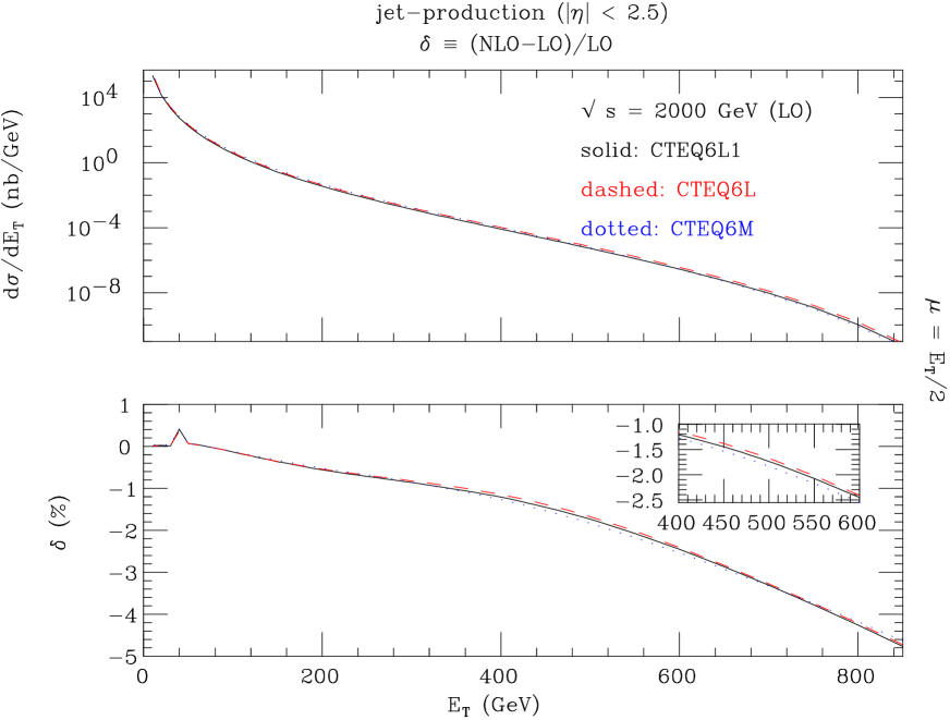
Figure 17: The effects of the ${\cal O}(\alpha_{\mathrm{S}}^{2}\alpha_{\mathrm{W}})$ corrections [bottom] relative to the full LO results (i.e., through ${\cal O}(\alpha_{\mathrm{S}}^{2}+\alpha_{\mathrm{S}}\alpha_{\mathrm{EW}}+\alpha_{\mathrm{EW}}^{2})$) [top] for the case of Tevatron (Run 2) for three choices of PDFs. They are plotted as function of the jet transverse energy $E_{T}$. The cut $|\eta|<2.5$ has been enforced, alongside the standard jet cone requirement $\Delta R>0.7$. The factorisation/renormalisation scale adopted was $\mu=\mu_{F}\equiv\mu_{R}=E_{T}/2$.

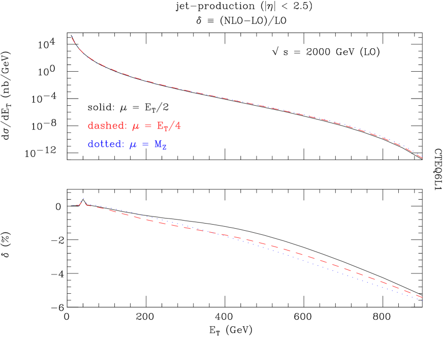
Figure 18: The effects of the ${\cal O}(\alpha_{\mathrm{S}}^{2}\alpha_{\mathrm{W}})$ corrections [bottom] relative to the full LO results (i.e., through ${\cal O}(\alpha_{\mathrm{S}}^{2}+\alpha_{\mathrm{S}}\alpha_{\mathrm{EW}}+\alpha_{\mathrm{EW}}^{2})$) [top] for the case of Tevatron (Run 2) for three choices of factorisation/renormalisation scale. They are plotted as function of the jet transverse energy $E_{T}$. The cut $|\eta|<2.5$ has been enforced, alongside the standard jet cone requirement $\Delta R>0.7$. The PDFs used were CTEQ6L1.

Here, we complement the results of [23] by studying the effects of the ${\cal O}(\alpha_{\mathrm{S}}^{2}\alpha_{\mathrm{W}})$ one-loop virtual corrections over the full kinematic range of the final state jets, rather than restrict ourselves to the specific case of published CDF and D0 data samples. Fig. 17 shows the size of the aforementioned corrections relative to the full LO results (as defined in the caption) for three sets of CTEQ PDFs [34] all taken at the factorisation/renormalisation scale $\mu=\mu_{F}\equiv\mu_{R}=E_{T}/2$, i.e., half the jet transverse energy, the standard choice in NLO QCD simulations (see Refs. [36]–[39]). Weak effects are basically independent of the PDFs used and results are negligible for small jet transverse energy, where the differential cross section is largest and therefore lead to negligible corrections in the integrated one. However, the corrections in the differential cross sections become somewhat relevant at large jet transverse energy. For example, at the kinematic end $E_{T}=800-900$ GeV they can reach the $-5\%$ level. It is however doubtful whether Tevatron can reach the luminosity necessary to isolate jets at such large jet transverse energies and even so it is most likely that such higher order effects will be overwhelmed by systematics. For the current highest reach of Run 2, $E_{T}\approx 650$ GeV, the ${\cal O}(\alpha_{\mathrm{S}}^{2}\alpha_{\mathrm{W}})$ effects studied here amount to only $-2.5\%$ for $\mu=E_{T}/2$. If one adopts another factorisation/renormalisation scale (see Fig. 18), they can be slightly larger. They increase in excess of $-3\%$ for $\mu=E_{T}/4$. For a fixed scale, e.g., $\mu=M_{Z}$, they reach $-4\%$. Notice however that for higher jet transverse energies the scale dependence reduces considerably. Of more relevance numerically is the case when the LO term is defined to be only of ${\cal O}(\alpha_{\mathrm{S}}^{2})$. As discussed in [23], for certain choices of $\mu$, the cumulative effect of EW corrections through ${\cal O}(\alpha_{\mathrm{S}}\alpha_{\mathrm{EW}}+\alpha_{\mathrm{EW}}^{2}+\alpha_{\mathrm{S}}^{2}\alpha_{\mathrm{W}})$ could well reach the $-10$ to $-15\%$ level for $E_{T}$ values which will be measurable within Run 2, with the tree-level and one-loop EW terms being of similar size. Thus, it is of paramount importance to establish which terms are included in Monte Carlo (MC) programs used to interpolate the data.

Clearly, in the case of Tevatron, the aforementioned logarithmic effects bring very little enhancement, as the $E_{T}$ values that can be probed at such a machine are not much larger than $M_{W}$ and $M_{Z}$. Therefore, despite through ${\cal O}(\alpha_{\mathrm{S}}^{2}\alpha_{\mathrm{W}})$ there are many more diagrams available for channels yielding two jets in the final state than via ${\cal O}(\alpha_{\mathrm{S}}^{2})$ or indeed ${\cal O}(\alpha_{\mathrm{S}}\alpha_{\mathrm{EW}})$ and ${\cal O}(\alpha_{\mathrm{EW}}^{2})$, the fact that the Sudakov regime is not reached here implies that the size of the corrections to the LO terms of ${\cal O}(\alpha_{\mathrm{S}}^{2})$ is never much larger than ${\cal O}(\alpha_{\rm W})$ (i.e., with no logarithmic enhancement). Besides, at FNAL energies, jet production is always dominated by quark-antiquark induced channels, so that large corrections typical of processes via quark-quark/antiquark-antiquark scattering (see later on) do not contribute much to the hadronic cross section.

5 LHC phenomenology

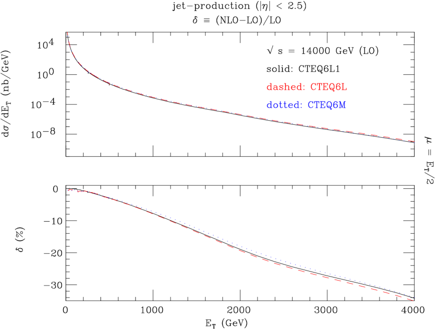
Figure 19: The effects of the ${\cal O}(\alpha_{\mathrm{S}}^{2}\alpha_{\mathrm{W}})$ corrections [bottom] relative to the full LO results (i.e., through ${\cal O}(\alpha_{\mathrm{S}}^{2}+\alpha_{\mathrm{S}}\alpha_{\mathrm{EW}}+\alpha_{\mathrm{EW}}^{2})$) [top] for the case of LHC for three choices of PDFs. They are plotted as function of the jet transverse energy $E_{T}$. The cut $|\eta|<2.5$ has been enforced, alongside the standard jet cone requirement $\Delta R>0.7$. The factorisation/renormalisation scale adopted was $\mu=\mu_{F}\equiv\mu_{R}=E_{T}/2$.

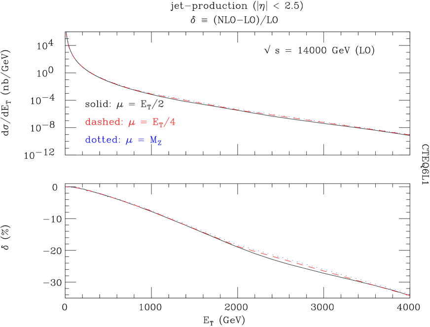
Figure 20: The effects of the ${\cal O}(\alpha_{\mathrm{S}}^{2}\alpha_{\mathrm{W}})$ corrections [bottom] relative to the full LO results (i.e., through ${\cal O}(\alpha_{\mathrm{S}}^{2}+\alpha_{\mathrm{S}}\alpha_{\mathrm{EW}}+\alpha_{\mathrm{EW}}^{2})$) [top] for the case of LHC for three choices of factorisation/renormalisation scale. They are plotted as function of the jet transverse energy $E_{T}$. The cut $|\eta|<2.5$ has been enforced, alongside the standard jet cone requirement $\Delta R>0.7$. The PDFs used were CTEQ6L1.

More dramatic results are found at LHC energies. Here, the jet transverse energy can be very large so that the corrections now include the Sudhakov enhancement. Furthermore, there is a considerable increase in quark-quark/antiquark-antiquark luminosity which, owing to the large number of four-fermion Feynman diagrams through one-loop (with respect to tree-level), increases significantly the impact of ${\cal O}(\alpha_{\mathrm{S}}^{2}\alpha_{\mathrm{W}})$ terms. We observe that the additional Feynman diagrams generally interfere constructively. For example, in our diagonal CKM matrix approximation, processes (9)–(10) only count one Feynman diagram at tree-level (via gluon exchange) whereas at one-loop they are mediated by all graphs depicted in Fig. 8. As some of the one-loop amplitudes are Sudakov-enhanced and some others are not and none of them is gauge-invariant on its own, it is not however possible to quantify a priori the overall impact of the increased number of graphs even channel by channel. In general, the larger the number of Sudakov-enhanced amplitudes the larger the corrections are. There is, however, a contrasting effect for the LHC due to the fact that gluon induced processes become dominant and these are generally subject to small weak corrections. This affects the overall normalisation but not the Sudakov enhancement. Altogether, despite the fact that the correction to the total cross section is still small, the corrections to the differential one at large $E_{T}$ are substantial, e.g., at $E_{T}=1$ TeV one-loop effects are already about $-10\%$ and increase further, up to $-35\%$ at 4 TeV, irrespective of the PDFs used (over most of the kinematical range): see Fig. 19. Also notice that the change of factorisation/renormalisation scale has a smaller impact at LHC than at Tevatron, as confirmed by Fig. 20.

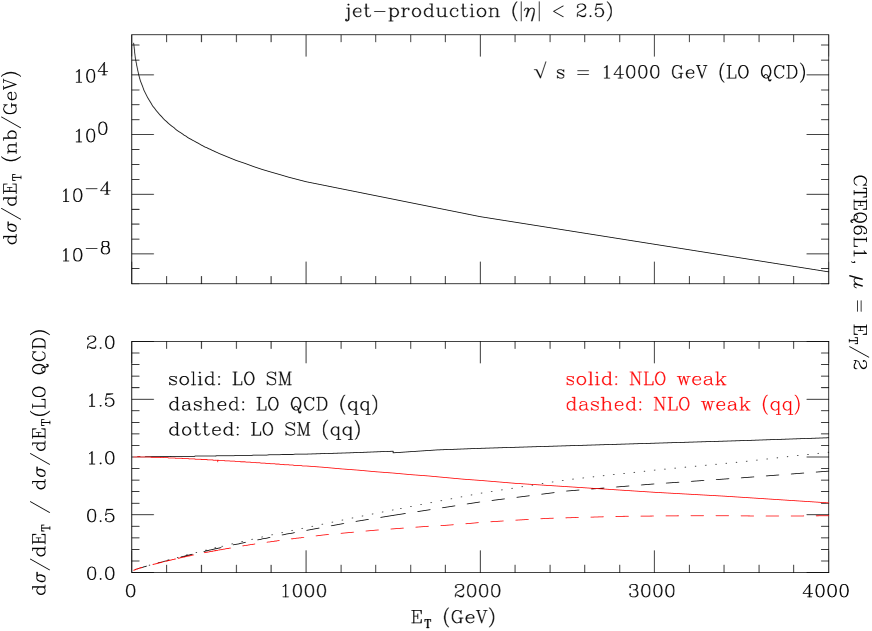
Figure 21: Top: The total single jet inclusive distribution in transverse energy through ${\cal O}(\alpha_{\mathrm{S}}^{2})$ at the LHC. Bottom: The effects of the one-loop ${\cal O}(\alpha_{\mathrm{S}}^{2}\alpha_{\mathrm{W}})$ and tree-level ${\cal O}(\alpha_{\mathrm{S}}\alpha_{\mathrm{EW}}+\alpha^{2}_{\mathrm{EW}})$ corrections relative to the spectrum above. The label (qq) refers to the case of subprocesses with no gluons in the initial state. Rates are plotted as function of the jet transverse energy $E_{T}$. The cut $|\eta|<2.5$ has been enforced, alongside the standard jet cone requirement $\Delta R>0.7$. The PDFs used were CTEQ6L1 whilst the factorisation/renormalisation scale adopted was $\mu=\mu_{F}\equiv\mu_{R}=E_{T}/2$.

The shape of the corrections in the Figs. 19 and 20 can be understood in terms of the partonic composition of the complete ${\cal O}(\alpha_{\mathrm{S}}^{2}\alpha_{\mathrm{W}})$ sample, distinguishing between processes initiated by (anti)quarks only and those which have a gluon component in the initial state, see Fig. 21. This distinction stems from the fact that in the case of subprocesses initiated by (anti)quarks only, one also has LO EW effects through ${\cal O}(\alpha_{\rm{S}}\alpha_{\mathrm{EW}}+\alpha_{\mathrm{EW}}^{2})$. (In the plot, the label LO SM identifies the sum of terms of ${\cal O}(\alpha_{\mathrm{S}}^{2}+\alpha_{\mathrm{S}}\alpha_{\mathrm{EW}}+\alpha_{\mathrm{EW}}^{2})$.) These, however, can only reach a $3\%$ effect at $E_{T}=1$ TeV, with respect to the ${\cal O}(\alpha_{\rm{S}}^{2})$ terms (LO QCD) and a $16\%$ effect at $E_{T}=4$ TeV. On the other hand, the ${\cal O}(\alpha_{\mathrm{S}}^{2}+\alpha_{\mathrm{S}}^{2}\alpha_{\mathrm{W}})$ terms (labelled NLO weak) lead to corrections up to $-40\%$ in the vicinity of 4 TeV, and even at $E_{T}=1$ TeV they amount to $-12\%$. Thus we observe that the one-loop corrections of order $\alpha_{\rm{S}}^{2}\alpha_{\mathrm{W}}$ dominate the tree-level interferences of order $\alpha_{\rm{S}}\alpha_{\mathrm{EW}}$ owing to the large logarithms. Finally, the plot also shows the contributions from only those subprocesses that are not initiated by any gluons (denoted by the label (qq)): it is clear that at very large $E_{T}$ (the Sudakov regime) are these channels that dominate much of the jet phenomenology.

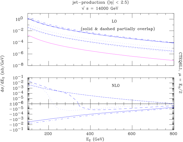
(c)

Figure 22: The total single jet inclusive distribution in transverse energy through tree-level (LO) via ${\cal O}(\alpha_{\mathrm{S}}^{2})$, ${\cal O}(\alpha_{\mathrm{S}}\alpha_{\mathrm{EW}})$ and ${\cal O}(\alpha_{\mathrm{EW}}^{2})$ (top) and one-loop (NLO) corrections at ${\cal O}(\alpha_{\mathrm{S}}^{2}\alpha_{\mathrm{W}})$ at the LHC. The cut $|\eta|<2.5$ has been enforced, alongside the standard jet cone requirement $\Delta R>0.7$. The PDFs used were CTEQ6L1 whilst the factorisation/renormalisation scale adopted was $\mu=\mu_{F}\equiv\mu_{R}=E_{T}/2$. Absolute rates are given for each of the suprocesses (1)–(15), labelled as follows (round brakets imply summation over corresponding channels):

It is also of interest to understand the different behaviours of the ${\cal O}(\alpha_{\mathrm{S}}^{2}\alpha_{\mathrm{W}})$ effects in terms of each of the partonic channels involved. To this end, we present Fig. 22(a)–(c), showing the contributions to the $E_{T}$ dependent cross section of subprocesses (1)–(15) (plus $gg\to gg$, $qq^{\prime}\to QQ^{\prime}$, $\bar{q}\bar{q}^{\prime}\to\bar{Q}\bar{Q}^{\prime}$ and $q\bar{q}^{\prime}\to Q\bar{Q}^{\prime}$ at LO only) separately at the LHC. We show the range from $E_{T}=$100 GeV, which is sufficiently far from poorly modelled threshold effects at $E_{T}\approx M_{W}/2$, to $E_{T}=$800 GeV, where Sudakov effects start being active in the ${\cal O}(\alpha_{\mathrm{S}}^{2}\alpha_{\mathrm{W}})$ corrections. The main purpose of this plot is to illustrate that, at the LHC, unlike the case of the Tevatron, the magnitude of the gluon luminosity inside the proton leads to gluon-initiated processes that can easily compete with the (anti)quark-initiated ones, even at rather large jet transverse energies. In fact, at LO, processes (3), (4) and $gg\to gg$ dominate over the total of the (anti)quark-initiated ones for all $E_{T}$ values considered in the plot. Tab. 1 quantifies this, e.g., at $E_{T}=800$ GeV. The ${\cal O}(\alpha_{\mathrm{S}}^{2}\alpha_{\mathrm{W}})$ corrections are particularly large for subprocesses (7)–(8), mainly by virtue of the large number of diagrams involved at loop level (as intimated earlier), with respect to the full LO case. Process (12) has a large positive correction. This can be understood from the fact that here the tree-level interference between strong and weak interactions is forbidden by colour and the leading contribution comes from a gluon exchanged in the $s$-channel. However, at one-loop level the cross section is substantially enhanced by the interference between a $t$-channel $W$-exchange and a $t$-channel gluon exchange, with a further gluon exchanged in the $t$-channel in order to conserve colour. Nevertheless this process only makes a small contribution to the complete jet sample. Altogether, despite the fact that corrections to individual channels can be of a few tens of percent, the overall ${\cal O}(\alpha_{\mathrm{S}}^{2}\alpha_{\mathrm{W}})$ effect is approximately $-6\%$, with respect to the ${\cal O}(\alpha_{\mathrm{S}}^{2}\alpha_{\mathrm{S}}\alpha_{\mathrm{EW}}+\alpha_{\mathrm{EW}}^{2})$. Similar patterns for the corrections are typical also at larger jet transverse energies, with the overall size of the one-loop corrections increasing steadily like $\sim\log^{2}(E_{T}^{2}/M_{W}^{2})$ or $\sim\log^{2}(E_{T}^{2}/M_{Z}^{2})$ and the quark-(anti)quark initiated processes gradually becoming dominant.

6 Summary and conclusion

In summary, whilst at the Tevatron ${\cal O}(\alpha_{\mathrm{S}}^{2}\alpha_{\mathrm{W}})$ one-loop virtual corrections to the single jet inclusive cross section may be comparable to statistical and systematic effects, at the LHC such terms are important contributions at large jet transverse energies. For the expected highest reach of the CERN machine (assuming standard luminosity), $E_{T}\approx 4$ TeV, they can be as large as an astounding $-35$ to $-40\%$ (depending on whether these are related to the LO QCD cross section or to the total tree-level one including interference between strong and EW interactions and the square of the latter). Therefore, they ought to be included in any comparison of theory with data in these regimes. However, particular care should be paid to the treatment of real $W$- and $Z$-production and decay in the definition of the inclusive jet data sample, as this will determine whether $W$- and $Z$-bremsstrahlung effects have to be included in the theoretical predictions through ${\cal O}(\alpha_{\mathrm{S}}^{2}\alpha_{\mathrm{W}})$, which might counterbalance the negative effects due to the one-loop $W$- and $Z$-exchange estimated here [33]. (As these were not included in our calculation, the matter is currently under study [45].)

Along the same lines, it should be recalled that NNLO EW terms ought to be investigated too, as it is well known from the Sudakov treatment that they may well be sizable in comparison to the NLO ones (see, e.g., Ref. [72]).

Our results on weak corrections to the single jet inclusive cross section at hadron colliders are in line with the findings in several other hadronic processes and in various approximations (see Refs. [46]–[71] for an incomplete list limited to the SM). Altogether they should help to raise the awareness that LHC physics (primarily) is not always dominated by QCD effects, particularly in extreme kinematic regimes where new physics beyond the SM could manifest itself, possibly in observables that are parity violating, hence sensitive to genuine (i.e., of SM origin) EW corrections but not QCD ones. In our view, progress in evaluating higher order QCD effects should proceed hand-in-hand with that of assessing similar EW effects.

7 Appendix

7.1 Helicity amplitudes

It is convenient to consider the virtual corrections in terms of helicity amplitudes. This approach has a number of advantages:

1. Contributions from individual Feynman graphs can be added to the helicity amplitudes numerically. This allows flexibility for different analyses of the various terms entering the virtual corrections as well as a higher degree of control of the correctness of the results (as more internal tests can be enforced).

2. The interference with the tree-level amplitudes can also be computed numerically. This avoids the cumbersome algebraic expressions that would be obtained if all possible interferences were computed analytically.

3. For applications in which it is possible to polarise the incoming beams (e.g., at the Relativistic Heavy Ion Collider (RHIC) [22]), the contributions from different helicity combinations can be matched with the corresponding polarised PDFs.

The formalism adopted for the case of subprocesses with external gluons, processes (1)–(4) in Sect. 2, has already been described in Refs. [21, 73] (see also [73, 74]). For the case of all other channels, processes (5)–(19) in Sect. 2 (including the bremsstrahlung contributions), we have found it convenient to adopt a different procedure. In order to describe this, let us consider, as an example, the amplitude ${\cal A}^{(s)}(s,t,\lambda_{1},\lambda_{2},\lambda_{3},\lambda_{4})$, where $\lambda_{1},\dots\lambda_{4}$ are the helicities of the incoming and outgoing partons as indicated below. For process (13) of Sect. 2:

$$q(p_{1},\lambda_{1})\,+\,\bar{q}(p_{2},\lambda_{2})\ \to\ Q(p_{3},\lambda_{3})\,+\,\bar{Q}(p_{4},\lambda_{4}),$$ (21)

where $q$ and $Q$ are quarks of different generations (recall that, as mentioned elsewhere, to the accuracy to which we are working it is safe to neglect CKM mixing of flavours in the weak interactions) and $p_{i}$ ($i=1,...4$) their four-momenta.

The contribution to the amplitude for this process from any Feynman graph must be of the form

$${\cal A}^{(s)}(s,t,\lambda_{1},\lambda_{2},\lambda_{3},\lambda_{4})\ =\ \bar{v}(p_{2},\lambda_{2})\Gamma_{1}u_{(}p_{1},\lambda_{1})\bar{u}(p_{3},\lambda_{3})\Gamma_{2}v_{(}p_{4},\lambda_{4})\delta_{\lambda_{1},-\lambda_{2}}\delta_{\lambda_{3},-\lambda_{4}},$$ (22)

where $\Gamma_{1},\ \Gamma_{2}$ contain strings of $\gamma$-matrices (as well as propagators and an implied integral over loop momentum). They are in general tensorial with indices contracted between $\Gamma_{1}$ and $\Gamma_{2}$. Since we are interested in energy scales which are much larger than the mass of the $b$-quark (and we are not considering $t$-quark production here), the quarks may be taken to be massless. In this case the strings of $\gamma$-matrices in $\Gamma_{1},\ \Gamma_{2}$ are vectors for self-energy or vertex correction diagrams and two-rank tensors for box diagrams. They may be reduced so that the most general forms are

$$\bar{v}(p_{2},\lambda_{2})\Gamma_{1}u_{(}p_{1},\lambda_{1})\ =\ a_{1}(s,t,\lambda_{1})A_{1}(s,\lambda_{1})\delta_{\lambda_{1},-\lambda_{2}}\,+\,b_{1}(s,t,\lambda_{1})B_{1}(s\lambda_{1})\delta_{\lambda_{1},-\lambda_{2}},$$ (23)

with

$$A_{1}(s,\lambda_{1})\ =\ \bar{v}(p_{2},\lambda_{2})\gamma\cdot w_{1}u_{(}p_{1},\lambda_{1})\ =\ \sqrt{s}$$ (24)

and

$$B_{1}(s,\lambda_{1})\ =\ \bar{v}(p_{2},\lambda_{2})\gamma\cdot nu_{(}p_{1},\lambda_{1})\ =\ i\lambda_{1}\sqrt{s},$$ (25)

where

$$w_{1}^{\mu}\ =\ {{1}\over{\sqrt{stu}}}\left(up_{1}^{\mu}+tp_{2}^{\mu}+sp_{3}^{\mu}\right)$$ (26)

is a unit vector in the scattering plane orthogonal to $p_{1}$ and $p_{2}$ and $n^{\mu}$ is a unit vector normal to the scattering plane.

The coefficients $a_{1}(s,t,\lambda_{1})$ and $b_{1}(s,t,\lambda_{1})$ have the same tensorial structure as $\Gamma_{1}$ and can be obtained by taking traces with the appropriate projection operators, i.e.,

$$a_{1}(s,t,\lambda_{1}) = {{1}\over{2}}{\mathrm{Tr}}\left(\Gamma_{1}\gamma\cdot w_{1}{{(1-\lambda_{1}\gamma^{5})}\over{2}}\right),$$

$$b_{1}(s,t,\lambda_{1}) = {{1}\over{2}}{\mathrm{Tr}}\left(\Gamma_{1}\gamma\cdot n{{(1-\lambda_{1}\gamma^{5})}\over{2}}\right).$$ (27)

The general form for $\bar{u}(p_{3},\lambda_{3})\Gamma_{2}v_{(}p_{4},\lambda_{4})$ is obtained similarly

$$\bar{u}(p_{3},\lambda_{3})\Gamma_{2}v_{(}p_{4},\lambda_{4})\ =\ a_{2}(s,t,\lambda_{3})A_{2}(s,\lambda_{3})\delta_{\lambda_{3},-\lambda_{4}}\,+\,b_{2}(s,t,\lambda_{1})B_{2}(s\lambda_{3})\delta_{\lambda_{3},-\lambda_{4}},$$ (28)

where

$$A_{2}(s,\lambda_{3})\ =\ \bar{u}(p_{3},\lambda_{3})\gamma\cdot w_{2}v_{(}p_{4},\lambda_{4})\ =\ -\sqrt{s}$$ (29)

and

$$B_{2}(s,\lambda_{3})\ =\ \bar{u}(p_{3},\lambda_{3})\gamma\cdot nv_{(}p_{4},\lambda_{4})\ =\ i\lambda_{3}\sqrt{s},$$ (30)

with

$$w_{2}^{\mu}\ =\ {{1}\over{\sqrt{stu}}}\left(tp_{3}^{\mu}+up_{4}^{\mu}+sp_{2}^{\mu}\right).$$ (31)

The contribution to the complete helicity amplitude from any graph can therefore be specified in terms of the coefficients $a_{1},b_{1},a_{2},b_{2}$.

For example, consider the tree-level graph contributing to process (13) in eq. (21) due to the exchange of a $Z$-boson,

In Feynman gauge, we set $\Gamma_{1}=\gamma^{\mu}$ and $\Gamma_{2}=\gamma_{\mu}$, and multiply the entire graph by

$$F\ =\ g^{Z}_{q,\lambda_{1}}g^{Z}_{Q,\lambda_{3}}{{1}\over{(s-M_{Z}^{2}+i\Gamma_{Z}M_{Z})}},$$

where $g^{Z}_{q,\lambda_{1}}\ g^{Z}_{Q,\lambda_{3}}$ are the couplings of the $Z$ to the quarks $q$ and $Q$, respectively. We find

$$a_{1} = Fw_{1}^{\mu},$$

$$b_{1} = Fn^{\mu},$$

$$a_{2} = Fw_{2\mu},$$

$$b_{2} = Fn_{\mu},$$ (32)

so that the contribution to the helicity matrix element is

$${\cal A}\ =\ Fs\left(w_{1}^{\mu}+n^{\mu}\right)\left(-w_{2\mu}+n_{\mu}\right)\ =\ g^{Z}_{q,\lambda_{1}}g^{Z}_{Q,\lambda_{3}}{{1}\over{(s-M_{Z}^{2}+i\Gamma_{Z}M_{Z})}}\left[s+2t+s\lambda_{1}\lambda_{3}\right].$$ (33)

The large set of Feynman graphs which contribute to any elementary process can be classified in terms of a small number of prototype graphs. The prototype graphs for process (21) are listed in the next section along with their contributions to the helicity matrix element.

For the case of quark-antiquark annihilation in which the quarks $q$ and $Q$ are of the same flavour (or at least the same generation), there will also be contributions to the helicity matrix element from graphs involving the exchange of gauge bosons in $t$-channel. The contribution from such graphs can be obtained by crossing symmetry from the graphs with the gauge bosons exchanged in $s$-channel,

$${\cal A}^{(t)}(s,t,\lambda_{1},\lambda_{2},\lambda_{3}\lambda_{4})\ =\ -{\cal A}^{(s)}(t,s,\lambda_{1},-\lambda_{3},\lambda_{2}-\lambda_{4}).$$ (34)

Similarly, once we have the helicity matrix element for quark-antiquark annihilation, the amplitudes for quark-quark or antiquark-antiquark scattering can be obtained using the usual crossing relations.

7.2 Individual topologies

In this subsection we display the contributions to the total helicity amplitude of process (13) in eq. (21). The graphs are calculated in Feynman gauge in the $\overline{\rm{DR}}$ scheme. Both IR and UV poles have been subtracted using a common subtraction scale, $\mu$. A generic mass $M$ is here attributed (for illustration purposes only) to all massive internal gauge bosons. Finally, all coupling constants and colour factors have been set to unity (we indicate the appropriate colour factor in cases where there may be a sign ambiguity). Notice that the forthcoming contributions have the same overall phase as the tree-level amplitude given in eq. (33).

7.2.1 Self-energy graphs

The contribution to the amplitude from a graph with a self-energy correction due to a massive gauge boson (mass $M$) on an external leg

is

$${{1}\over{16\pi^{2}}}\left\{{{1}\over{2}}+\ln\left({{M^{2}}\over{\mu^{2}}}\right)\right\}\left[1+{{2t}\over{s}}+\lambda_{1}\lambda_{3}\right].$$ (35)

The contribution to the amplitude from a graph with a gluon loop on the internal gluon line

is

$$-{{1}\over{16\pi^{2}}}{{5}\over{3}}\ln\left({{-s}\over{\mu^{2}}}\right)\left[1+{{2t}\over{s}}+\lambda_{1}\lambda_{3}\right].$$ (36)

(Here, the relevant colour factor is $C_{A}$.)

The contribution to the amplitude from a graph with a fermion-loop self-energy correction to an internal gluon line

is

$${{1}\over{16\pi^{2}}}{{4}\over{3}}\ln\left({{-s}\over{\mu^{2}}}\right)\left[1+{{2t}\over{s}}+\lambda_{1}\lambda_{3}\right].$$ (37)

(Here, the relevant colour factor is $T_{R}$.)

7.2.2 Vertex graphs

The contribution to the amplitude from a correction to a vertex due to a massless gauge boson

is

$${{1}\over{16\pi^{2}}}\left\{-\ln^{2}\left({{-s}\over{\mu^{2}}}\right)+3\ln\left({{-s}\over{\mu^{2}}}\right)+7\right\}{{s}\over{(s-M^{2})}}\left[1+{{2t}\over{s}}+\lambda_{1}\lambda_{3}\right].$$ (38)

The contribution to the amplitude from a correction to a gluon vertex due to a massless gauge boson with triple gauge-boson coupling

is

$$-{{1}\over{16\pi^{2}}}\left\{\ln\left({{-s}\over{\mu^{2}}}\right)-1\right\}\left[1+{{2t}\over{s}}+\lambda_{1}\lambda_{3}\right].$$ (39)

The convention for the triple gauge-boson coupling has been chosen such that the colour factor associated with this graph is $C_{A}$.

The contribution to the amplitude from a correction to a QCD vertex due to a massive gauge boson

is

$${{1}\over{16\pi^{2}}} \times \left\{\left(3+{{2M^{2}}\over{s}}\right)\left[\ln\left({{-s}\over{M^{2}}}\right)-1\right]-\ln\left({{M^{2}}\over{\mu^{2}}}\right)+{{2}\over{s^{2}}}(s+M^{2})^{2}\left[{{\pi^{2}}\over{6}}-{\mathrm{Li_{2}}}\left(1+{{s}\over{M^{2}}}\right)\right]\right\}$$ (40)

$$\times \left[1+{{2t}\over{s}}+\lambda_{1}\lambda_{3}\right],$$

where

$${\mathrm{Li_{2}}}(x)\ =\ {\mathrm{dilog}}(1-x)\ =\ -\int_{0}^{x}{{\ln(1-y)}\over{y}}dy.$$ (41)

We have assumed here that all the quark masses are negligible. In the case where the outgoing quarks are $b$-quarks and the gauge boson in the loop is a $W$ though, the internal quark is a $t$-quark, whose mass must be taken into consideration. In such cases the contribution to the amplitude is not readily expressed as an analytic function and the contribution is calculated numerically using Veltman-Passarino reduction [75] and the FF library [76].

7.2.3 Box graphs

The contribution to the amplitude from the box graph with two massless gauge bosons exchanged in $s$-channel

is

$${{1}\over{16\pi^{2}}} \times \Bigg{\{}{{t}\over{s}}\left[4\pi^{2}-4\ln^{2}\left({{-s}\over{\mu^{2}}}\right)+8\ln\left({{s}\over{t}}\right)\ln\left({{-s}\over{\mu^{2}}}\right)\right]$$ (42)

$$+ (1+\lambda_{1}\lambda_{3})\Bigg{[}-{{s}\over{u}}\pi^{2}+4\ln\left({{s}\over{t}}\right)\ln\left({{-s}\over{\mu^{2}}}\right)-\left(2+{{s}\over{u}}\right)\ln^{2}\left({{s}\over{t}}\right)$$

$$- 2\ln\left({{s}\over{t}}\right)-2\ln^{2}\left({{-s}\over{\mu^{2}}}\right)\Bigg{]}\Bigg{\}}.$$

The contribution to the amplitude from the box graph with a massless and a massive gauge boson exchanged in $s$-channel

is

$${{1}\over{4\pi^{2}(s-M^{2})}} \times \Bigg{\{}-4{{tM^{2}}\over{s}}\ln\left(1-{{s}\over{M^{2}}}\right)\ln\left({{M^{2}-s}\over{\mu^{2}}}\right)-4t\ln\left({{-t}\over{M^{2}}}\right)\ln\left(1-{{s}\over{M^{2}}}\right)$$ (43)

$$+ 2t\ln\left({{-t}\over{M^{2}}}\right)\ln\left(1+{{t}\over{M^{2}}}\right)-t\ln^{2}\left({{-t}\over{\mu^{2}}}\right)$$

$$- 4t\left(1+{{s}\over{M^{2}}}\right){\mathrm{Li_{2}}}\left({{s}\over{M^{2}}}\right)+2t{\mathrm{Li_{2}}}\left({{-t}\over{M^{2}}}\right)$$

$$+ (1+\lambda_{1}\lambda_{3})\Bigg{[}-2M^{2}\ln\left(1-{{s}\over{M^{2}}}\right)\ln\left({{M^{2}-s}\over{\mu^{2}}}\right)-{{(s-M^{2})}\over{s}}\ln\left(1-{{s}\over{M^{2}}}\right)$$

$$- {{s}\over{2}}\ln^{2}\left({{-t}\over{\mu^{2}}}\right)+\left({{(s-M^{2})^{2}}\over{u}}-2M^{2}\right)\ln\left({{-t}\over{M^{2}}}\right)\ln\left({{M^{2}-s}\over{t+M^{2}}}\right)$$

$$- s\ln\left({{-t}\over{M^{2}}}\right)\ln\left(1+{{t}\over{M^{2}}}\right)+(s-M^{2})\ln\left({{-t}\over{M^{2}}}\right)$$

$$+ \left({{(s-M^{2})^{2}}\over{u}}-4M^{2}\right)\left[{\mathrm{Li_{2}}}\left({{s}\over{M^{2}}}\right)-{\mathrm{Li_{2}}}\left({{-t}\over{M^{2}}}\right)\right]$$

$$- \left(s+2M^{2}\right){\mathrm{Li_{2}}}\left({{-t}\over{M^{2}}}\right)\Bigg{]}\Bigg{\}}.$$

Note that the terms containing $u$ in the denominator are always multiplied by a coefficient that vanishes when $s=-t$, so that there is no bogus singularity in the backward direction. The contributions from box graphs in which the two gauge bosons are crossed in $s$-channel may be obtained from the above box contributions by using the substitutions $t\leftrightarrow u$ and $\lambda_{3}\rightarrow-\lambda_{3}$. In the end, all virtual corrections to all partonic processes with external quarks and/or anti-quarks can be obtained from these prototype graphs and expressions by multiplying by the appropriate couplings and colour factors and by using the appropriate crossing relations. For reason of space we do not report here all such results. Rather, we make available upon request the codes that implement them.

Acknowledgements

SM thanks Joey Huston, Nigel Glover, Denis Comelli and Paolo Ciafaloni for useful discussions. All authors acknowledge useful email exchanges and discussions with Robert Thorne.

Figure 1: The set of interferences that contributes to process 1 ($gg\rightarrow q\bar{q}$) and, if we reverse the direction of time, 2 ($q\bar{q}\rightarrow gg$).

Figure 2: Continuing the set of interferences that contribute to process 1 ($gg\rightarrow q\bar{q}$) and, if we reverse the direction of time, 2 ($q\bar{q}\rightarrow gg$).

Figure 3: The set of interferences that contribute to process 3 ($qg\rightarrow qg$) and, if we reverse the direction of the fermion arrow, 4 ($\bar{q}g\rightarrow\bar{q}g$).

Figure 4: Continuing the set of interferences that contribute to process 3 ($qg\rightarrow qg$) and, if we reverse the direction of the fermion arrow, 4 ($\bar{q}g\rightarrow\bar{q}g$).

Figure 5: The set of interferences that contributes to process 5 ($qq\rightarrow qq$) and 6 ($\bar{q}\bar{q}\rightarrow\bar{q}\bar{q}$), the latter obtained by reversing the arrows on all fermion lines of the former.

Figure 6: Continuing the set of interferences that contributes to process 5 ($qq\rightarrow qq$) and 6 ($\bar{q}\bar{q}\rightarrow\bar{q}\bar{q}$), the latter obtained by reversing the arrows on all fermion lines of the former.

Figure 7: The set of interferences that contributes to process 7 ($qQ\rightarrow qQ$ (same generation)) and 8 ($\bar{q}\bar{Q}\rightarrow\bar{q}\bar{Q}$ (same generation)), the latter obtained by reversing the arrows on all fermion lines of the former. Here, the weak couplings to the two fermion lines will be different, this means we cannot implement the last two interferences as a factor of 2 as we could in Figs. 1, 2.

Figure 8: The set of interferences that contributes to process 9 ($qQ\rightarrow qQ$ (different generation)) and 10 ($\bar{q}\bar{Q}\rightarrow\bar{q}\bar{Q}$ (different generation)), the latter obtained by reversing the arrows on all fermion lines of the former. Here, the weak couplings to the two fermion lines will be different, this means we cannot implement the last two interferences as a factor of 2 as we could in Figs. 1, 2.

Figure 9: The set of interferences that contributes to process 11 ($q\bar{q}\rightarrow q\bar{q}$).

Figure 10: The set of interferences that contributes to process 11 ($q\bar{q}\rightarrow q\bar{q}$): continued from Fig. 9.

Figure 11: The set of interferences that contributes to process 11 ($q\bar{q}\rightarrow q\bar{q}$): continued from Figs. 9 and 10.

Figure 12: The set of interferences that contributes to process 12 ($q\bar{q}\rightarrow Q\bar{Q}$ (same generation)).

Figure 13: The set of interferences that contributes to process 13 ($q\bar{q}\rightarrow Q\bar{Q}$ (different generation)).

Figure 14: The set of interferences that contributes to process 14 ($q\bar{Q}\rightarrow q\bar{Q}$ (same generation)).

Figure 15: The set of interferences that contributes to process 15 ($q\bar{Q}\rightarrow q\bar{Q}$ (different generation)).

Figure 16: The interferences that contribute to process 16 (diagrams with a $Z$ exchange, $qg\rightarrow qq\bar{q}$) and 18 (diagrams with a $W$ exchange, $qg\rightarrow qQ\bar{Q}$). If we reverse the direction of the incoming fermion line we also obtain process 17 ($\bar{q}g\rightarrow\bar{q}\bar{q}q$) and 19 ($\bar{q}g\rightarrow\bar{q}\bar{Q}Q$).

(a)

(b)

$${\rm{(a)}}~{}~{}~{}~{}~{}~{}~{}~{}~{}~{}gg \to q\bar{q}~{}({\rm{solid~{}black,~{}LO~{}\&~{}NLO}})$$

$${\rm{(a)}}~{}~{}~{}~{}~{}~{}~{}~{}~{}~{}q\bar{q} \to gg~{}({\rm{fine-dashed~{}black,~{}LO~{}\&~{}NLO}})$$

$${\rm{(a)}}~{}~{}~{}~{}~{}~{}q(\bar{q})g \to q(\bar{q})g~{}({\rm{dotted~{}black,~{}LO~{}\&~{}NLO}})$$

$${\rm{(a)}}~{}~{}~{}~{}~{}~{}~{}~{}~{}~{}gg \to gg~{}({\rm{dashed~{}black,~{}LO~{}only}})$$

$${\rm{(b)}}~{}~{}~{}~{}~{}~{}~{}~{}~{}~{}qq \to qq~{}({\rm{solid~{}red,~{}LO~{}\&~{}NLO}})$$

$${\rm{(b)}}~{}~{}~{}~{}~{}~{}~{}~{}~{}~{}\bar{q}\bar{q} \to \bar{q}\bar{q}~{}({\rm{fine-dashed~{}red,~{}LO~{}\&~{}NLO}})$$

$${\rm{(b)}}~{}~{}~{}~{}~{}~{}~{}~{}~{}qQ \to qQ~{}({\rm{same~{}generation}})~{}({\rm{dotted~{}red,~{}LO~{}\&~{}NLO}})$$

$${\rm{(b)}}~{}~{}~{}~{}~{}~{}~{}~{}~{}\bar{q}\bar{Q} \to \bar{q}\bar{Q}~{}({\rm{same~{}generation}})~{}({\rm{dashed~{}red,~{}LO~{}\&~{}NLO}})$$

$${\rm{(b)}}~{}~{}~{}~{}~{}~{}~{}~{}~{}qQ \to qQ~{}({\rm{different~{}generation}})~{}({\rm{dot-dashed~{}red,~{}LO~{}\&~{}NLO}})$$

$${\rm{(b)}}~{}~{}~{}~{}~{}~{}~{}~{}~{}\bar{q}\bar{Q} \to \bar{q}\bar{Q}~{}({\rm{different~{}generation}})~{}({\rm{wide-dotted~{}red,~{}LO~{}\&~{}NLO}})$$

$${\rm{(c)}}~{}~{}~{}~{}~{}~{}~{}~{}~{}~{}q\bar{q} \to q\bar{q}~{}({\rm{solid~{}blue,~{}LO~{}\&~{}NLO}})$$

$${\rm{(c)}}~{}~{}~{}~{}~{}~{}~{}~{}~{}~{}q\bar{q} \to Q\bar{Q}~{}({\rm{same~{}generation}})~{}({\rm{fine-dashed~{}blue,~{}LO~{}\&~{}NLO}})$$

$${\rm{(c)}}~{}~{}~{}~{}~{}~{}~{}~{}~{}~{}q\bar{q} \to Q\bar{Q}~{}({\rm{different~{}generation}})~{}({\rm{dotted~{}blue,~{}LO~{}\&~{}NLO}})$$

$${\rm{(c)}}~{}~{}~{}~{}~{}~{}~{}~{}~{}q\bar{Q} \to q\bar{Q}~{}({\rm{same~{}generation}})~{}({\rm{dashed~{}blue,~{}LO~{}\&~{}NLO}})$$

$${\rm{(c)}}~{}~{}~{}~{}~{}~{}~{}~{}~{}q\bar{Q} \to q\bar{Q}~{}({\rm{different~{}generation}})~{}({\rm{dot-dashed~{}blue,~{}LO~{}\&~{}NLO}})$$

$${\rm{(c)}}~{}q(\bar{q})q^{\prime}(\bar{q}^{\prime}) \to Q(\bar{Q})Q^{\prime}(\bar{Q}^{\prime})~{}({\rm{wide-dotted~{}blue,~{}LO~{}only}})$$

$${\rm{(c)}}~{}~{}~{}~{}~{}~{}~{}~{}~{}q\bar{q}^{\prime} \to Q\bar{Q}^{\prime}~{}({\rm{solid~{}purple,~{}LO~{}only}})$$

$\sqrt{s}=14$ TeV, $E_{T}=800$ GeV

Subprocess	(a)	(b)	(c)
$gg\to gg$			14.3
(1)	–0.0292	–3.88	0.643
(2)	–0.0189	–3.97	0.408
(3)–(4)	–1.089	–1.75	53.2
(5)–(6)	–1.078	–9.36	9.85
(7)–(8)	–2.78	–23.9	9.93
(9)–(10)	–0.239	–6.68	3.07
(11)	–0.169	–5.82	2.48
(12)	0.0390	33.9	0.0985
(13)	–0.0274	–8.09	0.290
(14)	–0.0861	–2.98	2.47
(15)	–0.239	–6.69	3.05
$qq^{\prime}\to QQ^{\prime}$ or $\bar{q}\bar{q}^{\prime}\to\bar{Q}\bar{Q}^{\prime}$			0.0616
$q\bar{q}^{\prime}\to Q\bar{Q}^{\prime}$			0.00239
Total	–5.71

Table 1: The contributions of subprocesses (1)–(15) to the total correction through ${\cal O}(\alpha_{\mathrm{S}}^{2}\alpha_{\mathrm{W}})$ with respect to the full LO result, i.e., through ${\cal O}(\alpha_{\mathrm{S}}^{2}+\alpha_{\mathrm{S}}\alpha_{\mathrm{EW}}+\alpha_{\mathrm{EW}}^{2})$, in the case of the differential cross section at LHC for $E_{T}=800$ GeV. Column (a) indicates the percentage contribution of the correction to the total; column (b) indicates the percentage correction to the individual partonic process; column (c) indicates the percentage contribution from that partonic process at tree-level to the differential cross section. Here, we have paired together the channels with identical Feynman diagram topology. The cut $|\eta|<2.5$ has been enforced, alongside the standard jet cone requirement $\Delta R>0.7$. The PDFs used were CTEQ6L1 whilst the factorisation/renormalisation scale adopted was $\mu=\mu_{F}\equiv\mu_{R}=E_{T}/2$.

References

- [1] W. Hollik et al., Acta Phys. Polon. B35 (2004) 2533.
- [2] M. Ciafaloni, P. Ciafaloni and D. Comelli, Phys. Rev. Lett. 84 (2000) 4810, Nucl. Phys. B589 (2000) 359, Phys. Rev. Lett. 87 (2001) 211802.
- [3] M. Melles, Phys. Rept. 375 (2003) 219.
- [4] A. Denner, arXiv:hep-ph/0110155.
- [5] A. Denner and S. Pozzorini, Eur. Phys. J. C18 (2001) 461, Eur. Phys. J. C21 (2001) 63.
- [6] P. Taxil and J. M. Virey, Phys. Lett. B404 (1997) 302.
- [7] P. Taxil and J. M. Virey, Phys. Rev. D55 (1997) 4480.
- [8] P. Taxil and J. M. Virey, Phys. Lett. B441 (1998) 376.
- [9] P. Taxil and J. M. Virey, Phys. Lett. B383 (1996) 355.
- [10] F. Abe et al. [CDF Collaboration], Phys. Rev. D45 (1992) 1448.
- [11] S. Catani, Yu. L. Dokshitzer, M. H. Seymour and B. R. Webber, Nucl. Phys. B406 (1993) 187.
- [12] S. D. Ellis and D. E. Soper, Phys. Rev. D48 (1993) 3160.
- [13] M. H. Seymour, Z. Phys. C62 (1994) 127.
- [14] S. Bethke, Z. Kunszt, D. E. Soper and W. J. Stirling, Nucl. Phys. B370 (1992) 310 [Erratum-ibid. B523 (1998) 681].
- [15] Yu. L. Dokshitzer, G. D. Leder, S. Moretti and B. R. Webber, JHEP 9708 (1997) 001.
- [16] S. Moretti, L. Lonnblad and T. Sjostrand, JHEP 9808 (1998) 001.
- [17] S. D. Ellis, J. Huston and M. Tonnesmann, in Proc. of the APS/DPF/DPB Summer Study on the Future of Particle Physics (Snowmass 2001) ed. N. Graf, eConf C010630 (2001) P513.
- [18] F. Abe et al. [CDF Collaboration], Phys. Rev. Lett. 79 (1997) 2192.
- [19] M. Cveti, S. Godfrey, hep-ph/9504216; A. Leike, Phys. Rept. 317 (1999) 143.
- [20] F. Gianotti et al., Eur. Phys. J. C39 (2005) 293.
- [21] J. R. Ellis, S. Moretti and D. A. Ross, JHEP 0106 (2001) 043.
- [22] S. Moretti, M. R. Nolten and D. A. Ross, arXiv:hep-ph/0509254.
- [23] S. Moretti, M. R. Nolten and D. A. Ross, arXiv:hep-ph/0503152.
- [24] S. Moretti, M. R. Nolten and D. A. Ross, in arXiv:hep-ph/0604120.
- [25] U. Baur, E. W. N. Glover and A. D. Martin, Phys. Lett. B232 (1989) 519.
- [26] C. Bourrely, J. P. Guillet and J. Soffer, Nucl. Phys. B361 (1991) 72.
- [27] J. A. M. Vermaseren, arXiv:math-ph/0010025.
- [28] J. Kublbeck, M. Bohm and A. Denner, Comput. Phys. Commun. 60 (1990) 165.
- [29] P. Ciafaloni and D. Comelli, private communication.
- [30] S. Catani and M. H. Seymour, Nucl. Phys. B485 (1997) 291 [Erratum-ibid. B510 (1997) 503].
- [31] J. Pumplin, D. R. Stump, J. Huston, H. L. Lai, P. Nadolsky and W. K. Tung, JHEP 0207 (2002) 012.
- [32] G.P. Lepage, J. Comput. Phys. 27 (1978) 192 and Cornell preprint CLNS 80-447, March 1980.
- [33] P. Ciafaloni and D. Comelli, arXiv:hep-ph/0604070.
- [34] See http://durpdg.dur.ac.uk/hepdata/cteq.html.
- [35] T. Affolder et al. [CDF Collaboration], Phys. Rev. D64 (2001) 032001 [Erratum-ibid. D65 (2002) 039903].
- [36] F. Aversa, P. Chiappetta, M. Greco and J. P. Guillet, Phys. Lett. B210 (1988) 225, Phys. Lett. B211 (1988) 465, Nucl. Phys. B327 (1989) 105.
- [37] R. K. Ellis and J. C. Sexton, Nucl. Phys. B269 (1986) 445.
- [38] S. D. Ellis, Z. Kunszt and D. E. Soper, Phys. Rev. Lett. 64 (1990) 2121.
- [39] W. T. Giele, E. W. N. Glover and D. A. Kosower, Phys. Rev. Lett. 73 (1994) 2019.
- [40] H. L. Lai et al., Phys. Rev. D55 (1997) 1280.
- [41] D. Stump, J. Huston, J. Pumplin, W. K. Tung, H. L. Lai, S. Kuhlmann and J. F. Owens, JHEP 0310 (2003) 046.
- [42] http://www-cdf.fnal.gov/physics/new/qcd/inclusive/; http://www-d0.fnal.gov/Run2Physics/qcd/.
- [43] R. S. Thorne, talk given at the ‘HERA-LHC Workshop’, DESY, 21-24 March 2005; J. Huston, talk given at the ‘Physics at TeV Colliders workshop’, Les Houches, 2-20 May 2005; R. S. Thorne, A. D. Martin, R. G. Roberts and W. J. Stirling, AIP Conf. Proc. 792 (2005) 365.
-
[44]
T. Kluge, K. Rabbertz and M. Wobisch, in preparation (see:
http://hepforge.cedar.ac.uk/fastnlo/). - [45] J. Campbell, J. Huston, S. Moretti and D. A. Ross, in preparation.
- [46] W. Beenakker, A. Denner, W. Hollik, R. Mertig, T. Sack and D. Wackeroth, Nucl. Phys. B411 (1994) 343.
- [47] C. Kao, G. A. Ladinsky and C. P. Yuan, Int. J. Mod. Phys. A12 (1997) 1341.
- [48] U. Baur, S. Keller and D. Wackeroth, Phys. Rev. D59 (1999) 013002.
- [49] C. Kao and D. Wackeroth, Phys. Rev. D61 (2000) 055009.
- [50] U. Baur and D. Wackeroth, Int. J. Mod. Phys. A16S1A (2001) 326.
- [51] U. Baur, O. Brein, W. Hollik, C. Schappacher and D. Wackeroth, Phys. Rev. D65 (2002) 033007.
- [52] S. Dittmaier and M. Kramer, Phys. Rev. D65 (2002) 073007.
- [53] J. H. Kühn, S. Moch, A. A. Penin and V. A. Smirnov, Nucl. Phys. B616 (2001) 286.
- [54] S. Pozzorini, arXiv:hep-ph/0201077.
- [55] A. Denner, M. Melles and S. Pozzorini, Nucl. Phys. B662 (2003) 299.
- [56] E. Maina, S. Moretti, M. R. Nolten and D. A. Ross, Phys. Lett. B570 (2003) 205.
- [57] M. L. Ciccolini, S. Dittmaier and M. Kramer, Phys. Rev. D68 (2003) 073003.
- [58] E. Maina, S. Moretti, M. R. Nolten and D. A. Ross, arXiv:hep-ph/0401093.
- [59] E. Maina, S. Moretti, M. R. Nolten and D. A. Ross, arXiv:hep-ph/0407150.
- [60] W. Hollik and C. Meier, Phys. Lett. B590 (2004) 69.
- [61] E. Maina, S. Moretti and D. A. Ross, Phys. Lett. B593 (2004) 143.
- [62] U. Baur and D. Wackeroth, Phys. Rev. D70 (2004) 073015.
- [63] J. H. Kuhn, A. Kulesza, S. Pozzorini and M. Schulze, Phys. Lett. B609 (2005) 277.
- [64] E. Accomando, A. Denner and A. Kaiser, Nucl. Phys. B706 (2005) 325.
- [65] M. Beccaria, F. M. Renard and C. Verzegnassi, arXiv:hep-ph/0405036.
- [66] M. Beccaria, F. M. Renard and C. Verzegnassi, Phys. Rev. D71 (2005) 033005.
- [67] M. Beccaria, G. Macorini, F. M. Renard and C. Verzegnassi, arXiv:hep-ph/0605108.
- [68] M. Beccaria, G. Macorini, F. M. Renard and C. Verzegnassi, Phys. Rev. D73 (2006) 093001.
- [69] J. H. Kuhn, A. Scharf and P. Uwer, Eur. Phys. J. C45 (2006) 139.
- [70] W. Bernreuther, M. Fucker and Z. G. Si, Phys. Lett. B633 (2006) 54, Int. J. Mod. Phys. A21 (2006) 914.
- [71] S. Moretti, M. R. Nolten and D. A. Ross, arXiv:hep-ph/0603083.
- [72] P. Ciafaloni and D. Comelli, Phys. Lett. B476 (2000) 49; V. S. Fadin, L. N. Lipatov, A. D. Martin and M. Melles, Phys. Rev. D61 (2000) 094002; W. Beenakker and A. Werthenbach, Nucl. Phys. B630 (2002) 3; A. Denner, M. Melles and S. Pozzorini, Nucl. Phys. B662 (2003) 299; B. Feucht, J. H. Kuhn, A. A. Penin and V. A. Smirnov, Phys. Rev. D93 (2004) 101802; B. Jantzen, J. H. Kuhn, A. A. Penin and V. A. Smirnov, Phys. Rev. D72 (2005) 051301.
- [73] E. Maina, S. Moretti and D. A. Ross, JHEP 0304 (2003) 056.
- [74] E. Maina, S. Moretti and D. A. Ross, arXiv:hep-ph/0403269.
- [75] G. Passarino and M. J. G. Veltman, Nucl. Phys. B160 (1979) 151.
- [76] G. J. van Oldenborgh and J. A. M. Vermaseren, Z. für Phys. C46 (1990) 425.