A Theory of Cosmic Rays

Abstract

We present a theory of non-solar cosmic rays (CRs) in which the bulk of their observed flux is due to a single type of CR source at all energies. The total luminosity of the Galaxy, the broken power-law spectra with their observed slopes, the position of the ‘knee(s)’ and ‘ankle’, and the CR composition and its variation with energy are all predicted in terms of very simple and completely ‘standard’ physics. The source of CRs is extremely ‘economical’: it has only one parameter to be fitted to the ensemble of all of the mentioned data. All other inputs are ‘priors’, that is, theoretical or observational items of information independent of the properties of the source of CRs, and chosen to lie in their pre-established ranges. The theory is part of a ‘unified view of high-energy astrophysics’ —based on the ‘Cannonball’ model of the relativistic ejecta of accreting black holes and neutron stars. The model has been extremely successful in predicting all the novel properties of Gamma Ray Bursts recently observed with help of the Swift satellite. If correct, this model is only lacking a satisfactory theoretical understanding of the ‘cannon’ that emits the cannonballs in catastrophic processes of accretion.

I Introduction and outlook

The field of cosmic-ray (CR) physics was born as a lucky failure. The 1912 attempt by Victor Hess to measure the decrease of the Earth’s radioactivity in an ascending balloon gave an opposite result: there was an extra-terrestrial source of what are now known to be high-energy nuclei and electrons. Almost a century later, the origin of non-solar CRs is still a subject of intense research and little consensus Reviews . We shall refer throughout to non-solar cosmic rays simply as CRs.

Over almost a century, an impressive set of CR data have been gathered, e.g. the all-particle spectrum (of nuclei, without distinction of charge and mass) has been measured over some 13 orders of magnitude in energy and more than 30 orders of magnitude in flux (perhaps only Coulomb’s law is measured over an even wider range). It has become standard practice to present the spectral data as the flux $dF/dE$ times a power of energy, which emphasizes the spectral ‘features’ and the discrepancies between experiments, while de-emphasizing the pervasive systematic errors in energy. The all-particle spectrum $E^{3}\,dF/dE$ is shown in Fig. 1 for energies $E>10^{11}$ eV. The figure shows that the spectrum is roughly describable as a broken power law Reviews ; Kampert ; HIRES1 :

$$\;\;\;\;\;\;\;\;\;\;\;\;\;\;{dF/dE}\propto E^{-\beta},$$

$$\beta \simeq 2.7;\;\;\;E<E[{\rm knee}]\sim 3\times 10^{15}\rm\;eV,$$

$$\beta \simeq 3.0;\;\;\;E[{\rm knee}]\,<\,E<\,E[{\rm knee2}]\sim 2\times 10^{17}\rm\;eV,$$

$$\beta \sim 3.1;\;\;\;E[{\rm knee2}]\,<\,E<\,E[{\rm ankle}],$$

$$\beta \sim 2.7;\;\;\;E>E[{\rm ankle}]\sim 3\times 10^{18}\rm\;eV.$$ (1)

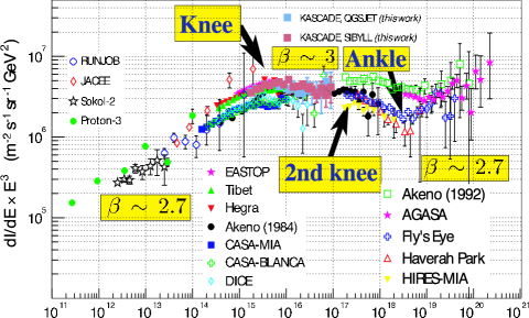
Figure 1: The all-particle CR spectrum wheighted by $E^{3}$, with its three changes of spectral index: the ‘knee’, the ‘second knee’, and the ‘ankle’ Kampert .

Below ${E[{\rm knee]}}$, protons constitute $\sim 96\%$ of the CRs at fixed energy per nucleon. Their flux above ${E_{p}\sim 10}$ GeV is Haino :

$${dF_{p}\over dE}\simeq{1.37\pm 0.13\over\rm cm^{2}~{}s~{}sr~{}GeV}\;\left[E\over\rm GeV\right]^{-2.73\pm 0.03}\,.$$ (2)

The conventional theory of CRs GP posits that supernova remnants are the site of acceleration of (non-solar) CRs for energies up to $E[{\rm knee}]$. No consensus on a preferred accelerator site or mechanism exists for energies between $E[{\rm knee}]$ and $E[{\rm ankle}]$. It has long being argued that CRs of energy above $E[{\rm ankle}]$ are extragalactic in origin Cocconi ; Morrison : they cannot be isotropized by the Galactic magnetic fields, but their observed arrival directions are isotropic HIRES2 . We refer to CRs with $E>E[{\rm ankle}]$ as ultra-high energy cosmic rays (UHECRs). They are the subject of great interest, considerable controversy and imaginative model-building; see, for instance, the review by J. Cronin in Reviews . In this paper we use many abbreviations. They are listed in Table 1.

Table 1: Frequently used abbreviations

Afterglow(s)	AG(s)
Active Galactic Nucleus(i)	AGN(s)
Cosmic Background Radiation	CBR
Cosmic Microwave Background	CMB
$[$Non-solar$]$ Cosmic Ray(s)	CR(s)
Cosmic-Ray Electron(s)	CRE(s)
Gamma Background Radiation	GBR
$[$Long-duration$]$ Gamma-Ray Burst(s)	GRB(s)
Inter-Galactic Medium	IGM
Inter-Stellar Medium	ISM
Inverse Compton Scattering	ICS
Greisen, Zatsepin & Kuzmin	GZK
Lorentz Factor(s)	LF(s)
Magnetic Field(s)	MF(s)
Short Hard [$\gamma$-ray] Burst(s)	SHBs
Starlight	SL
Superbubble(s)	SB(s)
Supernova(e)	SN(e)
Supernova Remnant(s)	SNR(s)
Synchrotron Radiation	SR
Ultra-High Energy Cosmic Ray(s)	UHECR(s)
X-Ray Flash(es)	XRF(s)

Radio, X-ray and $\gamma$-ray observations of supernova remnants (SNRs) provide clear evidence that electrons are accelerated to high energies in these sites. So far, they have not provided unambiguous evidence that SNRs accelerate CR nuclei and are their main source in any energy range Plaga . Moreover, SNRs cannot accelerate CRs to energies as large as $E[{\rm knee}]$ Hillas , though this point is still debated. A direct proof —such as a localized source— of an extragalactic origin of the UHECRs was lacking until very recently Reviews ; HIRES2 . The precise interpretation of the recent results of Auger PAC on the correlation of directions between UHECRs and Active Galactic Nuclei (AGNs), which we discuss in detail in Sections X.3 and X.4, may still be debatable.

There is mounting observational evidence that, in addition to the ejection of a non-relativistic spherical shell, the explosion of a core-collapse supernova (SN) results in the emission of highly relativistic bipolar jets of plasmoids of ordinary matter, Cannonballs. Evidence for the ejection of such jets in SN explosions is not limited to GRBs but comes also from optical observations of SN 1987A NP , from X-ray UH and infrared OK observations of Cassiopeia A and, perhaps, from the morphology of radio SNRs RNM . These jets may be the main source of CR nuclei at all energies DP ; DAD ; Florence . They also explain long-duration GRBs DETAL , as advocated in the CB model GRB1 ; DD .

In this paper we elaborate on a previous theory of CRs DP , which is very different from the conventionally accepted theories Reviews . For much of the required input, we exploit the subsequently acquired information provided by the CB-model analysis of long-duration $\gamma$-ray bursts (GRBs) and X-ray flashes (XRFs). The jets of CBs responsible for GRBs are akin to the jets of CBs emitted by quasars and microquasars. The former jets, we shall argue, are also responsible for the generation of CRs.

The essence of our considerations may be pictorially conveyed. The quasar Pictor A is shown in Fig. 2. The X-ray picture in the top panel shows one of its extremely narrow jets, which we interpret as X-ray emission from a jet of CBs. The lower panel shows the two opposite jets, and contour plots of their radio-emission fluence. We interpret the radio signal as the synchrotron radiation of ‘cosmic-ray’ electrons. Electrons and nuclei were scattered by the CBs, which encountered them at rest in the intergalactic medium (IGM), kicking them up to high energies. Thereafter, these particles diffuse in the ambient magnetic fields (MFs) and the electrons efficiently emit synchrotron radiation. In applying this picture to the CRs in our Galaxy, we will simply replace the quasar for all past Galactic and extragalactic core-collapse SNe, and fill in the details.

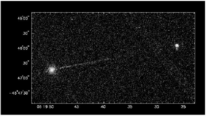
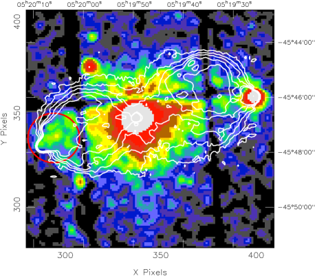
Figure 2: Top: X-ray image of the galaxy Pictor A. A non-expanding jet extends across 360000 light years towards a hot spot at least 800000 light years away from where the jet originates PG . Bottom: XMM/p-n image of Pictor A in the 0.2–12 keV energy interval, centred at the position of the leftmost spot in the upper panel, superimposed on the radio contours of a 1.4 GHz radio VLA map WYS .

As a CB from a core-collapse SN travels through the interstellar medium (ISM), it encounters ISM matter that has been previously ionized by the passage of the GRB’s $\gamma$ radiation. The CB’s density is low enough for individual interactions between its ionized plasma constituents and those of the ISM to be irrelevant. The ISM ions and electrons are only deflected by the collective effects of the CB’s inner MFs, generated by the very same ions and electrons. We shall see in detail that this makes a CB act as a formidably efficient relativistic magnetic-racket accelerator, which loses essentially all of its energy to the recoiling particles: the newly born CRs. We argue that this very simple concept explains all observed properties of non-solar CRs at all observed energies.

Cosmic-ray sources other than high-energy jets —such as the traditional expanding SN envelopes, novae, stellar flares, stellar winds and non-relativistic jets— may be relevant at low energies. Galactic high-energy CRs are also emitted by ordinary pulsars, by soft $\gamma$-ray repeaters, by microquasars, and probably in the final merger of neutron stars and black holes in binary systems. The total CR luminosity of these objects is smaller than the observed one by more than two orders of magnitude. Similar considerations lead us to neglect, or to discuss cum grano salis, the extragalactic contribution of relativistic jets from massive black holes in AGNs, perhaps the most luminous potentially competitive sources. These topics are discussed in Section X.4 and Appendix F.

Our predictions for the $E^{3}$-weighted fluxes of the most abundant nuclei and ‘groups’ of nuclei are shown in Fig. 3, which previews and summarizes our results. The source spectra are shown in Fig. 3a; two of their features are: ‘knees’ at energies proportional to the atomic number $A$; and ‘Larmor’ cutoffs (proportional to the nuclear charge $Z$) beyond which our CR acceleration mechanism is no longer operative. The CR spectra arriving to our planet are shown in Fig. 3b. The differences between these two figures —which are significant and will be discussed in minute detail— are due to the many ‘tribulations’ a CR suffers in travelling to Earth from the location of its source. Two examples of tribulations are:

(1) Below a certain momentum (some $3\times 10^{9}\;Z$ GeV/c) the local flux of CRs of Galactic origin is enhanced by a factor proportional to their momentum-dependent Galactic ‘confinement’ time Swordy :

$$\tau_{\rm conf}\propto\left({Z\,{\rm GeV/c}\over p}\right)^{\beta_{\rm conf}};\,\,\,\,\,\,\,{\beta_{\rm conf}}\sim 0.6\pm 0.10.$$ (3)

This is the origin of the differing slopes of the lower-energy fluxes in Figs. 3a,b (note their different scales).

(2) Extragalactic CRs other than protons are efficiently photo-dissociated by the cosmic background infrared radiation on their way to our Galaxy. This is part of the explanation for the very different relative abundances of the elements at the higher energies in Figs. 3a and 3b.

One can see in Fig. 3b how H and He dominate up to their knees, which add up to the knee feature of the all-particle spectrum; how the composition thereafter becomes ‘heavier’ and dominated by Fe up to its knee, which is the second knee of the all-particle spectrum; and how the flux becomes once again ‘lighter’ above this feature. The UHECRs are entirely extragalactic in origin and are dominantly protons.

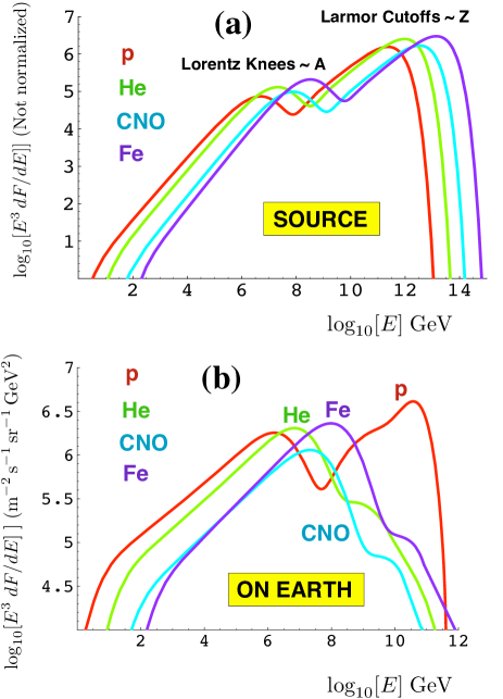
Figure 3: Predicted CR spectra for the most abundant elements and groups. The vertical scales are $E^{3}\,dF/dE$. (a): The source spectra, with a common arbitrary normalization. (b): The CR spectra at the location of the Earth. Notice that both the horizontal and vertical scales are different.

Ours is also a theory of CR electrons and of their radiative contribution to the diffuse $\gamma$ background radiation (GBR). The diffuse GBR at low Galactic latitudes originates mainly from $\pi^{0}$-generating collisions of CR nuclei with the ISM, followed by $\pi^{0}\to 2\gamma$ decay. At high Galactic latitudes the diffuse GBR, we contend DDGBR , is dominated by inverse-Compton radiation from CR electrons in the ISM and the halo of galaxies (including ours) and in the IGM. In this sense, CR nuclei, CR electrons and a good fraction of the diffuse GBR have the same origin Anton , the latter radiation being a CR ‘secondary’.

More specific results, to be derived in detail and in agreement with the data, are:

• The slope of the CR source spectra below the knees is predicted to be $\beta_{s}\simeq 2.17$, as derived in Section V.1. Modified by Galactic confinement, this corresponds to observed spectra with a slope $\beta_{s}+{\beta_{\rm conf}}\approx 2.77$, with ${\beta_{\rm conf}}$ as in Eq. (3).

• A very slight composition dependence of the slope of the source spectra is expected. This can be discerned in Fig. 3. It is discussed in Section V.3 and shown in Fig. 12.

• The CR spectra at the lowest energies are affected by solar effects. The predictions agree with the data at minimum solar activity; see Section V.10 and Fig. 16.

• The spectra of the individual CR nuclei are predicted to have ‘knees’, scaling as the atomic weight, at energies around $E[{\rm knee}]\!\sim\!3\!\times\!10^{15}\,A\,{\rm eV}$; see Eq. (34) and Figs. 3, 10. The observed and predicted spectra for the individual elements H, He and Fe, at energies up to their knees, are shown in Fig. 15.

• The CR spectrum is predicted to change rather abruptly in slope, dominant composition (Fe to H) and dominant origin (Galactic to extragalactic) at the ‘ankle’ energy, $E[{\rm ankle}]\sim 3\times 10^{18}\;{\rm eV}$, see Section V.7.

• Our CR acceleration mechanism has a cutoff at the energies of Eq. (39), proportional to atomic charge and roughly coincident with the conventional Greisen–Zatsepi–Kuzmin (GZK) cutoff GZK . These cutoffs do not seem to be present in the AGASA data AGASA , but are compatible with the HIRES HIRES2 , Fly’s Eyes’ and Auger Mello ; Unger ; PAC data, which agree well with our theory: see Fig. 13.

• The predicted normalization of the UHECR flux is approximate but ‘absolute’, i.e. parameter-free; see Section V.6.

• The prediction for the all-particle spectrum is compared with the data in Fig. 14.

• Detailed predictions for the ‘primary’ CR abundances relative to hydrogen are discussed in Section V.2. They are compared with data at 1 TeV in Table 2 and illustrated in Fig. 11.

• Data on two rough indicators of the evolution of CR composition with energy, $\langle\ln A\rangle$ and the depth of shower maximum $X_{\rm max}$, are compared with predictions in Figs. 17 and 18.

• The confinement volume and the confinement time of CRs in the Galaxy can be estimated theoretically. They agree with the estimates extracted from observations, as discussed in Section V.12.

• Below their respective knees, the source spectra of CR nuclei and electrons are predicted to have the same slope: $\beta_{s}=13/6$. For relatively high-energy electrons, radiation cooling steepens the slope to $\beta_{e}=\beta_{s}+1\sim 3.17$. The observed slope is $\simeq 3.2$, as shown in Fig. 21. The normalization of the electron spectrum, we cannot predict.

• The slope of the diffuse GBR is predicted to be $(\beta_{e}+1)/2\simeq 2.08$. The observation is $\simeq 2.1$, as shown in Fig. 22.

Admittedly, the ‘predictions’ we have referred to in the above items are ‘postdictions’ of existing data. Yet, the theory on which they are based is very ‘predictive’: only one parameter specific to the CR source will be fitted to the hadronic CR data. Otherwise, only priors (items of information independent of the CR source) have been used as inputs, and kept at their ‘central’ values, or within their error brackets cosmopriors .

The study of GRBs, some 40 years old, is in its infancy, if compared with the century-old study of CRs. In the GRB realm, novel and very precise data, in particular at X-ray energies and mainly thanks to the Swift satellite, are being gathered. The predictions of the CB model have been precisely verified by the data having appeared since our first posting of this paper in June 2006. This subject is very briefly summarized in Section X.1.

A posteriori the distinction between post- and pre-dictions, or parameters and priors, is somewhat artificial. But there are other assets of the CR theory presented here: it works simply and very well, and it is based on a single source of CR acceleration at all energies. Moreover, the underlying theory —originally inspired by an analogy with the relativistic ejecta of quasars and microquasars— is part of a unified model of high-energy astrophysical phenomena Florence , which also offers simple and successful explanations of the origin and properties of ‘long-duration’ GRBs and X-ray flashes and their respective afterglows (AGs) DD ; AGoptical ; AGradio ; DDDXRF , the natal kicks of neutron stars DP , the MFs and radio emission from within and near galaxy clusters DDMF , and the X-ray emission from galactic clusters allegedly harbouring ‘cooling flows’ CDD .

The many titles and subtitles in this paper should suffice to convey its organization. We discuss in detail or summarize in Appendices some of the relevant background information: how a CB expands, photo-dissociation, the least debatable ‘priors’ common to all theories of CRs, jets in astrophysics, the CB model, the evidence for the ejection of relativistic jets in SN explosions, the supernova–GRB association and the power supply by CR accelerators other than the one we propose.

Our main point is our proposed mechanism of CR acceleration. A reader primarily interested in it may choose to read first Section III.1 on ‘Collisionless magnetic rackets’. A reader primarily intrigued by the results may choose to start with Chapter V.

II CB priors

The ‘cannon’ of the CB model is analogous to the ones responsible for the ejecta of quasars and microquasars. As an ordinary core-collapse SN implodes into a black hole or neutron star and sheds an exploding shell, an accretion disk or torus is hypothesized to be produced around the newly born compact object, either by stellar material originally close to the surface of the imploding core and left behind by the explosion-generating outgoing shock, or by more distant stellar matter falling back after its passage ADR ; GRB1 ; DD . A CB is emitted, as observed in microquasars Felix ; DMR , when part of the accretion disk falls abruptly onto the compact object GRB1 ; DD .

In the case of a core-collapse SN, the accretion torus is not fed by a companion, it has a finite mass and can feed a limited number of accretion episodes. Each episode corresponds to the bipolar emission of a CB pair. A CB generates a forward cone of high-energy photons as its constituent electrons Compton-up-scatter ambient light. If the jet is directed close to the line of sight of an observer, each of its CBs generates a pulse in a GRB signal; a bit more off axis, an XRF is observed. The CBs, like the matter that feeds them from the accreting torus, are made of ordinary-matter plasma. The typical initial Lorentz factor (LF) of a CB, $\gamma_{0}$, and its typical initial baryon number, $N_{{}_{\rm B}}$, are DD :

$$\gamma_{0} \equiv E/(M_{0}\,c^{2})\sim{\cal{O}}(10^{3}),$$ (4)

$$N_{{}_{\rm B}} \sim 10^{50}.$$ (5)

The value of $M_{0}\sim N_{{}_{\rm B}}\,m_{p}\,c^{2}$ roughly corresponds to half of the mass of Mercury, a very small number in comparison with the mass of the parent exploding star. An artist’s view of the CB model is given in Fig. 4.

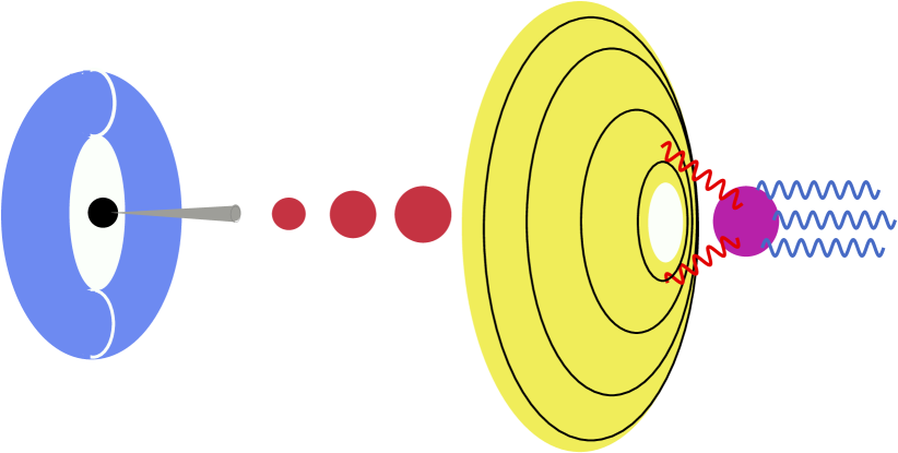
Figure 4: An ‘artist’s view” (not to scale) of the CB model of long-duration GRBs DD . A core-collapse SN results in a compact object and a fast-rotating torus of non-ejected fallen-back material. Matter (not shown) abruptly accreting into the central object produces a narrowly collimated beam of CBs, of which only some of the ‘northern” ones are depicted. As these CBs move through the ‘ambient light” surrounding the star, they Compton up-scatter its photons to GRB energies.

The CB model of GRBs and their AGs is briefly discussed in Appendix D. Some of the distributions and average values of the input priors required in our theory of CRs are specific to this model. They are summarized in this Section, along with the other ingredients of the CB model relevant to CR production.

II.1 The distribution of initial Lorentz factors

Let $\gamma_{0}$ denote the value of the LF of a CB as it is originally emitted by a SN and produces a GRB’s $\gamma$-ray pulse by inverse Compton scattering (ICS), before it is slowed down by the ISM while generating the GRB’s afterglow by synchrotron radiation. An average value $\overline{\gamma_{0}}\sim 10^{3}$ was first estimated using the rough hypothesis that an asymmetry between the momenta of the diametrically opposed jets was responsible for the ‘natal kick’ velocity of neutron stars, the remnants of the core-collapse SN explosions of relatively light progenitors DP . This value of $\overline{\gamma_{0}}$ was confirmed by a first study of GRBs GRB1 within the CB model. It is also compatible with the roughly 1 to 1 SN–GRB association discussed in Appendix D.3.

A subsequent analysis of GRB afterglows (AGs) at infrared and optical AGoptical as well as radio AGradio frequencies confirmed $\overline{\gamma_{0}}\sim 10^{3}$ as the average initial LF. The distribution of $\gamma_{0}$ values obtained from these analyses for the ensemble of GRBs of known redshift (as of 2002) is shown in Fig. 5, constructed with the results of Ref. AGradio . The figure refers to data obtained with the selection criteria for the detection of GRBs, which discriminates in favour of large LFs, and is the result of fits to AGs which —with the exception of some GRBs clearly dominated by two CBs— are made with the simplification of substituting an ensemble of CBs for a single ‘average’ one. This tends to make the extracted $\gamma_{0}$ distribution narrower than the ‘real’ one, and its real average somewhat uncertain.

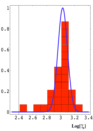
Figure 5: Distribution of $\log_{10}(\gamma_{0})$ values for GRBs of known redshift DD . The continuous curve is a log-normal fit.

The properties of CRs depend on the ‘real’ $\gamma_{0}$ distribution, which we parametrize as:

$$D(\gamma_{0},\overline{\gamma_{0}})\propto\exp\left[-\left({\log\gamma_{0}-\log\overline{\gamma_{0}}\over\log w}\right)^{2}\right].$$ (6)

The distribution of Fig. 5 has $\overline{\gamma_{0}}=1070$ and $\omega=0.8$. It results in a good description of CR data, but, not surprisingly, a somewhat broader distribution gives an even better description, as discussed in Section V.9. The predictions for CRs are insensitive to the assumed form of the lower-energy tail of $D(\gamma_{0},\bar{\gamma}_{0})$.

II.2 The deceleration of CBs in the ISM

While a CB exits from its parent SN and emits a GRB pulse, it is assumed GRB1 to be expanding, in its rest system, at a speed comparable to that of sound in a relativistic plasma ($v_{s}=c/\sqrt{3}$). In their voyage, CBs continuously intercept the electrons and nuclei of the ISM, previously ionized by the GRB’s $\gamma$-rays. In seconds of (highly Lorentz- and Doppler-foreshortened) GRB observer’s time, such an expanding CB becomes ‘collisionless’, that is, its radius becomes smaller than a typical interaction length between a constituent of the CB and an ISM particle. But a CB still interacts with the charged ISM particles it encounters, for, as we discuss in detail in Section II.5, it contains a strong magnetic field.

Consider a CB of initial mass $M_{0}$ and initial LF $\gamma_{0}$. As it travels in the ISM its LF diminishes all the way to unity. We assume that the ISM particles entering a CB’s magnetic mesh are trapped in it and slowly re-exit by diffusion. To a fair approximation, a CB simply accumulates the ISM particles that it intercepts. In this case, energy–momentum conservation implies that the CB’s mass increases as:

$$M_{\rm CB}\approx M_{0}\,{\gamma_{0}\over\beta\,\gamma},\;\;\;\;\left[\beta\equiv{\sqrt{\gamma^{2}-1}/\gamma}\right],$$ (7)

and, for an approximately hydrogenic ISM of local density $dn_{\rm in}$, the LF decreases as:

$${d\,\gamma\over\beta^{3}\,\gamma^{3}}\approx-\,{m_{p}\over M_{0}\,\gamma_{0}}\;dn_{\rm in}(\gamma).$$ (8)

To compute the spectrum of the CRs produced by a CB in its voyage through the ISM, we shall have to perform a $dn_{\rm in}$ integral over its trajectory, as the CB decelerates from $\gamma=\gamma_{0}$ to $\gamma=1$. Given Eq. (8), this is tantamount to integrating the CR spectra at local values of $\gamma$ with a weight factor $dn_{\rm in}\propto{d\gamma/(\gamma^{3}\,\beta^{3})}$. Notice that the CB’s deceleration law of Eq. (8) depends explicitly on the number of ISM particles it intercepts, but not on any CB properties other than $M_{0}$ and $\gamma_{0}$.

II.3 The expansion of a CB

We approximate a CB, in its rest system, by a sphere of radius $R(\gamma)$. The value of $R(\gamma_{0})$ is immaterial, for it becomes rapidly negligible as the CB initially expands at a speed $\sim c/\sqrt{3}$. The ISM particles that are intercepted —isotropized in the CB’s inner magnetic mesh, and re-emitted— exert an inwards force on it that, we assume, has as its main effect to counteract the CB’s expansion. This expansion, in the ‘fast elastic’ case of instantaneous re-emission, was studied in AGoptical ; AGradio . The case of ‘diffusive’ re-emission results in a slightly better description of more recent data DDDSwift . We discuss it in detail in Appendix A and we adopt it here.

The behaviour of $R(\gamma)$ is shown in Fig. 6. It has three distinct phases. The initial rapidly expanding quasi-inertial phase plays a crucial role in the description of GRB pulse shapes and is supported by the CB-model’s correct prediction of all their other properties DD . The properties of the intermediate coasting phase are supported by the CB-model’s successful description of GRB AGs; see, e.g. AGoptical ; AGradio ; DDDSwift . The final blow-up phase may describe the observed lobes of quasars and microquasars, such as the one at the right of Pictor A in Fig. 2.

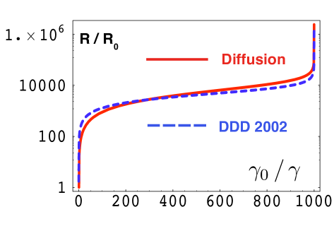
Figure 6: Expansion of a CB as its LF $\gamma$ diminishes along its trajectory from an initial $\gamma_{0}=10^{3}$. The dotted line is for the case of fast elastic CB interactions with the ISM, discussed in AGoptical ; AGradio . The continuous line is for the case discussed here, in which the ISM gathered by the CB slowly oozes out of it by diffusion. These are two limiting cases.

A CB converts the ISM into CRs at a rate proportional to $R_{{}_{\rm CB}}^{2}$. The initially fast-expanding phase in $R_{{}_{\rm CB}}(\gamma)$ has negligible effects. The subsequent behaviour of $R_{{}_{\rm CB}}(\gamma)$, in the diffusive case and for typical (or average) CB parameters, is well described by:

$$R_{{}_{\rm CB}}(\gamma) \approx R_{0}\,\left({\gamma_{0}\over\beta\,\gamma}\right)^{2/3},$$

$$R_{0} \sim 10^{14}\;{\rm cm}.$$ (9)

This behaviour gives the best description of GRB afterglows, as discussed in DDDSwift and Appendix A.

II.4 The trajectories of CBs

How far does a CB travel before the collisions with the ISM stop it? The answer crucially depends on the distribution of ISM densities that the CB encounters, and the relativistic approximation ($\beta\approx 1$) suffices to give it with the required precision. In the ‘slow’ approximation —in which the rate at which the ISM particles enter the CB is faster than the rate at which they exit it by diffusion— every ISM proton intercepted by a CB increases its mass by $\gamma\,m_{p}$. The mass increase per travel length $dx$ is:

$$dM_{{}_{\rm CB}}=\pi\,R_{{}_{\rm CB}}^{2}\,\gamma\,m_{p}\,n_{p}\,dx.$$ (10)

The relation between $dM_{{}_{\rm CB}}$ and $d\gamma$ is, according to Eq. (7), $\gamma\,dM_{{}_{\rm CB}}=M_{0}\,\gamma_{0}\,d\gamma/\gamma_{0}$, and $R_{{}_{\rm CB}}$ is given in Eq. (9). Gathering this information and integrating the result in $dx$ and $d\gamma$ we obtain:

$$x = x_{\rm stop}\,\left({1\over\gamma^{2/3}}-{1\over\gamma_{0}^{2/3}}\right),$$

$$x_{\rm stop} \equiv {3\,N_{{}_{\rm B}}\over 2\pi\,R_{0}^{2}\,\gamma_{0}^{1/3}}\;\bar{n}_{p}=(18\;{\rm kpc})\times$$ (11)

$$\!\!\!\!\!\!\!\!\!\!\!\!\left[{N_{{}_{\rm B}}\over 10^{50}}\right]\left[{10^{14}\,{\rm cm}\over R_{0}}\right]^{2}\left[{10^{-2}\,{\rm cm^{-3}}\over\bar{n}_{p}}\right]\left[{10^{3}\over\gamma_{0}}\right]^{1\over 3},$$

where $\bar{n}_{p}$, an adequately averaged ISM density along a given CB’s trajectory, is perhaps the most uncertain of the case-by-case varying inputs in $x_{\rm stop}$.

In the geometrically unlikely case that a CB travels in the plane of the Galaxy and crosses its central densest regions, its reach should be much less than the 18 kpc in Eq. (11). In the opposite extreme, if a CB exits perpendicularly to the plane of the Galaxy from a relatively high point in its ISM density distribution, it can reach beyond the Galactic halo into intergalactic space.

Cannonballs typically move from the inner SN-rich realm of the Galaxy into its halo or beyond and, along their trajectories, they convert into CRs the ISM particles they encounter, absorb and re-emit, as illustrated in Fig. 7. The CRs are forward-emitted by the fast-moving CBs, subsequently meandering in the Galactic MFs till they eventually escape the Galaxy.

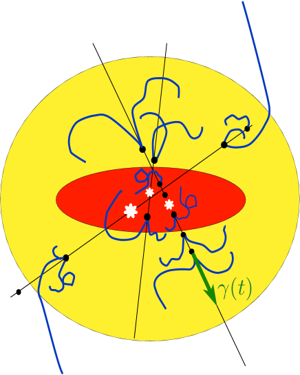
Figure 7: A schematic representation of the Galaxy and its halo. The CBs (black dots) emitted in the explosions of a few SNe are shown. All along their long straight trajectories (thin black lines), CBs slow down by collisions with the ISM, converting it into forward cones of CRs (blue lines), which curve on the magnetic fields of the Galaxy and its halo, eventually exuding into intergalactic space. The SN rate is such that an actual ‘snapshot’ should contain many more jets of CBs.

In our Galaxy SNe occur at a rate of about twice a century. This is a much shorter time than it takes a CB to travel over most of its trajectory, between a fraction of a kpc and several kpc, while still moving at a relativistic LF. Thus the Galaxy and its halo are, at any moment, permeated by scores of CB sources: Fig. 7 should show many more CB trajectories. A CB is a continuous source of CRs along its trajectory, and its source intensity depends on the local and previously traversed ISM density: in our theory the source of CRs is very diffuse. Thus, the directional anisotropy of CRs at the Earth’s location is expected to be very small and to vary little with energy, as observed Smith .

In models in which CRs diffuse away from point sources in the Galaxy’s disk, CR diffusion and hypothetical reacceleration mechanisms play a crucial role, particularly for CR electrons. In the CB model, on the contrary, CR transport by diffusion should not play a significant role, and reacceleration mechanisms need not be invoked.

II.5 The magnetic field within a CB

The ‘collisionless’ interactions of a CB and the ISM electrons and nuclei constitute the merger of two ordinary-matter plasmas at a large relative LF $\gamma$. This merger should be very efficient in creating turbulent currents and the consequent MFs within the CB, the denser of the two plasmas DP ; GRB1 . We assume that these MFs, as the CB reaches a quasi-stable radius, are in ‘equipartition’: their pressure (or energy density) equals the pressure exerted on the CB’s surface by the ISM particles it re-emits (or the energy density of the ISM particles it has temporarily phagocytized). This results in a time-dependent magnetic-field strength AGoptical :

$$B_{{}_{\rm CB}}[\gamma,n_{p}]=3\;{\rm G}\;{\gamma\over 10^{3}}\;\left({n_{p}\over 10^{-3}\;{\rm cm}^{-3}}\right)^{1/2}\;,$$ (12)

where $n_{p}$ is the ISM number density, normalized to a value characteristic of the ‘superbubbles’ (SB) in which most SNe and GRBs are born. The simple ensuing analysis of the elaborate time and frequency dependence of AGs —dominated by synchrotron radiation of electrons in the field of Eq. (12)— is very successful AGradio . Thus, we adopt the result of Eq. (12) in our analysis of CRs.

II.6 Fermi acceleration within a CB

Charged particles interacting with macroscopic, turbulently moving MFs, tend to gain energy: a ‘Fermi’ acceleration process. This acceleration is very efficient for a relativistic ‘injection’, the case relevant to a CB, which is subject, in its rest system, to a flow of ISM electrons and nuclei arriving with a large common LF. A ‘first-principle’ numerical analysis Fred of the merging of two plasmas at a moderately high $\gamma$ —based on following each particle’s individual trajectory as governed by the Lorentz force and Maxwell’s equations— demonstrates the generation of such chaotic MFs, and the acceleration of particles to a spectrum with a power-law tail:

$${dN_{\rm ac}\over dE}\sim E^{-\beta_{\rm ac}}\;\Theta(E-\gamma\,M\,c^{2}),\;\;\;\;\;\;\beta_{\rm ac}\approx 2.2.$$ (13)

The Heaviside $\Theta$ function is an approximate characterization of the fact that it is much more likely for the light particles to gain than to lose energy in their elastic collisions with the heavy ‘particles’ (the CB’s turbulently moving collective plasma and MF domains). The numerical analysis Fred shows that this acceleration occurs in a total absence of shocks, very much unlike what is generally assumed for CRs accelerated in shocks produced by expanding SN shells GP . In Fig. 8 we reproduce a plot of Fred showing the ion and electron currents at two depths into the denser of the merging plasmas.

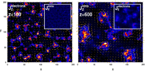
Figure 8: Results of a simulation of the merger of two plasmas at a relative LF $\gamma=3$. The left panel shows the longitudinal electron current density through a cut transverse to the direction of motion of the incoming plasma, with a small inset showing the ion current in the same plane. The right panel shows the ion current deeper into the target plasma, with the small inset now showing the electron current instead. The arrows represent the transverse magnetic field Fred .

In our analysis of the radio, infrared, optical, UV and X-ray AGs of GRBs, we assumed that a fraction of the ISM electrons entering a CB was accelerated as in Eq. (13), the majority remaining unaccelerated at their incoming LF. In the case of electrons, both populations ‘cool’ by synchrotron radiation in the CB’s MFs. The ensuing synchrotron radiation —the afterglow— has a complex frequency and time dependence, which is in excellent agreement with observations and —assuming that the index $\beta_{\rm ac}$ of Eq. (13) is the same for electrons and nuclei— confirms that Eqs. (12,13) are adequate; see Sections X.1 and D.6. The same index governs the high-energy tail of the “prompt” $\gamma$-ray and X-ray spectrum of GRBs, again in agreement with observations DD .

We assume that CR nuclei entering a CB from the ISM are also accelerated as in Eq. (13). This acceleration cannot extend to arbitrarily high energies; there must be a Larmor cutoff, for a CB has a finite radius and MF. A CB cannot significantly bend or accelerate a particle of energy larger than:

$$E[{\rm Larmor}]\simeq 9\times 10^{16}\;Z\;{\rm eV}\;{B_{{}_{\rm CB}}[\gamma_{0},n_{p}]\over 3\;{\rm G}}\;{R_{{}_{\rm CB}}\over 10^{14}\;{\rm cm}},$$ (14)

with $R_{{}_{\rm CB}}$ as in Eq. (9) and $B_{{}_{\rm CB}}$ as in Eq. (12). This corresponds to a maximum LF in the CB’s rest system:

$$\gamma_{\rm max}(\gamma)=b\;\gamma^{1/3}$$ (15)

$$b\simeq 10^{5}\;\gamma_{0}^{2/3}\;(Z/A).$$ (16)

The distribution of the LFs, $\gamma_{A}$, of the Fermi-accelerated nuclei that entered a CB with a Lorentz factor $\gamma$, is:

$${dN\over d\gamma_{{}_{A}}}\propto\gamma_{{}_{A}}^{-\beta_{\rm ac}}\,\Theta(\gamma_{{}_{A}}-\gamma)\,\Theta[\gamma_{\rm max}(\gamma)-\gamma_{{}_{A}}],$$ (17)

where the second $\Theta$ function is a rough characterization of the Larmor cutoff. But for the small dependence of the coefficient $b$ on the nuclear identity (the factor $Z/A$), the spectrum of Eq. (17) is universal.

II.7 The energy of the jets of CBs

The baryon number $N_{{}_{\rm B}}$ of a CB —or, equivalently, its mass $M\simeq N_{{}_{\rm B}}\,m_{p}$— can be roughly estimated from the fluence of the AG of GRBs AGoptical ; AGradio and better constrained from the ‘spherical-equivalent’ total energy and number of the $\gamma$-rays in a single GRB pulse DD . The average result is $N_{{}_{\rm B}}\sim 10^{50}$, cited in Eq. (5).

The observed average number Quilligan of significant pulses in a GRB’s $\gamma$-ray light curve is $\sim 6$. The total energy of the two jets of CBs in a GRB event is therefore:

$$E[{\rm jets}]\simeq 12\,\gamma_{0}\,N_{{}_{\rm B}}\,m_{p}\,c^{2}\simeq 2\!\times\!10^{51}\;\rm erg.$$ (18)

Practically all of this energy will, in our model, be transferred to CRs.

II.8 The CR luminosity of the Galaxy

In a steady state, if the low-energy rays dominating the CR luminosity are chiefly Galactic in origin, their accelerators must compensate for the escape of CRs from the Galaxy. The Milky Way’s luminosity in CRs must therefore satisfy:

$${L_{\rm CR}\simeq L_{p}={4\pi\over c}\int_{V_{\rm CR}}dV\int{dE\over\tau_{\rm conf}}\,E\,{dF_{p}\over dE}}\,,$$ (19)

with $dF_{p}/dE$ as in Eq. (2), $\tau_{\rm conf}$ as in Eq. (3), and ${V_{\rm CR}}$ the volume to which low-energy CRs are confined. The coefficient $1/\tau_{\rm conf}$, for $Z=1$, converts the observed proton spectrum into the corresponding source spectrum. The conventional result of detailed models of CR production and diffusion SM1 is:

$${L_{\rm CR}\sim 2\times 10^{41}\rm~{}erg~{}s^{-1}}\,.$$ (20)

Let $R_{\rm SN}$ be the SN rate in our Galaxy, discussed in Appendix B.3, and given by Eq. (95). The estimate of $L_{\rm CR}$ in the CB model is simply:

$$L_{\rm CR}{\rm[MW]}\!\approx\!R_{\rm SN}{\rm[MW]}\,E{\rm[jets]}\!\approx\!1.3\times 10^{42}\,\rm erg\,s^{-1},$$ (21)

with $E{\rm[jets]}$ as in Eq. (18). This estimate is uncertain by a factor of at least 2, for two reasons. First, SNe are observed to produce roughly spherical non-relativistic ejecta, whose kinetic energy is comparable to $E{\rm[jets]}$. The luminosity is dominated by low-energy CRs, which may also be produced —with debatable efficiency— by these ejecta, as in the generally accepted models. This may increase the result of Eq. (21) by a factor $\leq\!2$. Second, we contend DDMF that the MFs observed in the Milky Way and in galaxy clusters are generated by CRs, and are in energy equipartition with them, as observed in the Galaxy Longair , for which

$$\rho_{{}_{E}}{\rm[CR]}={4\,\pi\over c}\,\int{dF\over dE}\,E\,dE\approx 0.5\,\rm eV\,cm^{-3},$$ (22)

and

$${B^{2}/(8\,\pi)}\approx\rho_{{}_{E}}{\rm[CR]},\;\;\;\;\;\;{\rm for}\;B\sim 5\,\mu{\rm G}.$$ (23)

The transfer to MFs of $\sim$ 50% of the original CR energy may decrease the result of Eq. (21) by a factor $\sim\!2$ DSS .

III A theory of the CR source

III.1 Collisionless magnetic rackets

The essence of our theory of CRs is kinematical and trivial. A very massive object (a CB) travelling with a Lorentz factor $\gamma$ and colliding with a light object (an ISM particle) can boost the light object (now a CR) to extremely high energy.

By definition, in an elastic interaction of a CB at rest with ISM electrons or ions of LF $\gamma$, the light recoiling particles retain their incoming energy. Viewed in the system in which the ISM is at rest, the light recoiling particles (of mass $m$) have an energy spectrum extending, for large $\gamma$, up to $E\simeq 2\,\gamma^{2}\,m\,c^{2}$. A moving CB is a Lorentz-boost accelerator of gorgeous efficiency: the ISM particles it scatters reach up to $\gamma_{{}_{\rm CR}}\simeq 2\,\gamma^{2}$, with $\langle\gamma_{{}_{\rm CR}}\rangle\sim\gamma^{2}$ for any non-singular scattering-angle distribution in the CB’s rest system. In a single scattering with a CB of $\gamma\sim 10^{3}$, and with 100% efficiency, the energy of an ISM particle increases a million-fold from its value at rest. The ‘accelerator’ is also good at focusing: it produces a forward-collimated beam of CRs, the initial divergence of whose angular distribution is characterized by an angle $\theta\sim 1/\gamma$.

A particle with a LF $\gamma$ entering a CB at rest can be accelerated by elastic interactions with the CB’s turbulently moving plasma. Viewed in the rest system of the bulk of the CB the interaction is ‘inelastic’: the light particle gained energy. Its LF can reach $\gamma_{\rm max}\sim 10^{7}\,\gamma$; see Eqs. (15,16). Boosted by the CB’s motion the spectrum of the scattered particles extends to $\gamma_{{}_{\rm CR}}\sim 2\times 10^{7}\,\gamma^{2}$, in the UHECR domain, for $\gamma\sim\gamma_{0}\sim 10^{3}$. This powerful Fermi–Lorentz accelerator completes our theory of CRs.

We have tacitly assumed in the previous paragraph that interactions are instantaneous: a CB has the same LF when a given ISM particle enters and leaves it; the CB has not decelerated in the meantime via collisions with many other ISM nuclei. Borrowing from the language of particles more elementary than CBs, we called the interactions inelastic or elastic. In what follows we retract the cited assumption, but we keep the italicized nomenclature to refer to our results for particles that have —or have not— been Fermi-accelerated within a CB.

III.2 Exiting a CB by diffusion

Let $\gamma_{\rm in}$ be the LF of a given ISM proton that entered a CB. Its momentum stays fixed as it is tossed around by the CB’s inner chaotic magnetic field, or is increased by the acceleration mechanism we have discussed. For the ISM nuclei, as opposed to electrons, radiative and collisional losses are negligible. We assume that these trapped particles ooze out of the CB by diffusion, much as CRs do in the Galaxy. The characteristic diffusion time when the LF [radius] of the CB has reached a value $\gamma$ [$R_{{}_{\rm CB}}(\gamma)$] is:

$$\tau={R_{{}_{\rm CB}}^{2}\over D}\;,$$ (24)

with $D=D(\gamma_{\rm in},\gamma)$ a diffusion coefficient. The rate at which the diffusing particles are exuded by the CB is $r=\beta_{\rm in}/\tau$.

In the CB model, the MF of the Galaxy DDMF and that within a CB are both made by the same turbulence, induced by the injection of relativistic particles (the ISM in the case of a CB, CRs in the case of the Galaxy). Consequently, we expect $D$ to have the same energy dependence as observed for CRs: $D\propto p_{\rm in}^{\beta_{\rm conf}}$, with the same ${\beta_{\rm conf}}$ as in Eq. (3). In the case of a CB, the diffusion occurs in a MF with an energy density assumed to be in approximate equipartition with the kinetic energy density of the particles entering the CB at a given moment $B\propto\gamma-1$, and $D$ should reflect the $B$-, $A$- and $Z$-dependence of the corresponding Larmor radius, that is:

$$D\propto\left(E\over B\right)^{\beta_{\rm conf}}\propto\left[A\,\gamma_{\rm in}\over Z\,(\gamma-1)\right]^{\beta_{\rm conf}}.$$ (25)

The diffusion, out of a CB, of the fraction of ISM nuclei that are accelerated within it, will be treated in an entirely analogous fashion.

III.3 ‘Elastic’ scattering

We have assumed that, to a good approximation, a CB ingurgitates most of the ISM nuclei that it intercepts in its voyage, and that, within a CB, a fraction of these nuclei keeps the energy at which they entered it. In this approximation, and at the moment when the CB’s LF has descended from $\gamma_{0}$ to $\gamma$, the distribution of LFs, $\gamma_{\rm co}$, of the collected nuclei is:

$${dN_{\rm co}\over d\gamma_{\rm co}} = \int_{\gamma}^{\gamma_{0}}\,{dn_{\rm in}\over d\gamma_{\rm in}}\,\delta(\gamma_{\rm co}-\gamma_{\rm in})$$ (26)

$$\propto {1\over\beta_{\rm co}^{3}\,\gamma_{\rm co}^{3}}\;\Theta(\gamma\leq\gamma_{\rm co}\leq\gamma_{0}),$$

where we have used Eq. (8) and an unconventional but transparent notation for the Heaviside step function $\Theta$.

The collected particles exit the CB in its rest system at a rate $\beta_{\rm in}/\tau$, so that the doubly differential ($\gamma$, $\gamma_{\rm co}$) oozing out rate is:

$${dN_{\rm out}\over d\gamma\,d\gamma_{\rm co}}={dN_{\rm co}\over d\gamma_{\rm co}}\;{dt_{{}_{\rm CB}}\over d\gamma}\;{\beta_{\rm co}\over\tau}\;,$$ (27)

where

$$-{dt_{{}_{\rm CB}}\over d\gamma}\propto{1\over\beta^{4}\,\gamma^{4}\,R_{{}_{\rm CB}}^{2}}\;,$$ (28)

obtained by inserting

$$dn_{\rm in}(\gamma)\approx-\pi\,R_{{}_{\rm CB}}^{2}\,c\,n_{p}\,\beta\,\gamma\,dt_{{}_{\rm CB}}$$ (29)

into Eq. (8).

To specify the distribution of LFs, $\gamma_{{}_{\rm CR}}$, of the CRs in the ISM rest system, we must perform the corresponding boost over an assumed isotropic distribution of exit directions in the CB’s rest system:

$${dN_{\rm out}\over d\gamma_{{}_{\rm CR}}\,d\gamma\,d\gamma_{\rm co}}=$$

$$\int{d\cos\theta\over 2}{dN_{\rm out}\over d\gamma\,d\gamma_{\rm co}}\delta[\gamma_{{}_{\rm CR}}-\gamma\,\gamma_{\rm co}\,(1+\beta\,\beta_{\rm co}\,\cos\theta)].$$ (30)

The condition $|\cos\theta|\leq 1$ introduces two constraints which, solved for $\gamma_{\rm co}$, read:

$$\!\!\!\!\!\gamma_{\rm co} \leq T(\gamma,\gamma_{{}_{\rm CR}})\equiv\gamma\,\gamma_{{}_{\rm CR}}(1+\beta\,\beta_{{}_{\rm CR}}),$$

$$\!\!\!\!\!\gamma_{\rm co} \geq B(\gamma,\gamma_{{}_{\rm CR}})\equiv\gamma\,\gamma_{{}_{\rm CR}}(1-\beta\,\beta_{{}_{\rm CR}}).$$ (31)

To compute the CR flux $dF/d\gamma_{{}_{\rm CR}}$, we must integrate over $\gamma$ and $\gamma_{\rm co}$. Collecting all the results of this section and using Eqs. (9), (24) and (25), we obtain:

$${dF_{\rm elast}\over d\gamma_{{}_{\rm CR}}}\propto n_{{}_{A}}\beta_{{}_{\rm CR}}\left({A\over Z}\right)^{\beta_{\rm conf}}\int_{1}^{\gamma_{0}}{d\gamma\over(\beta\,\gamma)^{7/3}}\,{G[\gamma,\gamma_{{}_{\rm CR}}]\over(\gamma-1)^{\beta_{\rm conf}}}\;,$$

$$G[\gamma,\gamma_{{}_{\rm CR}}]\equiv\int_{\rm max(\gamma,B)}^{\rm min(\gamma_{0},T)}{\beta_{\rm co}\,d\gamma_{\rm co}\over(\beta_{\rm co}\,\gamma_{\rm co})^{4-{\beta_{\rm conf}}}}\;,$$ (32)

where we have introduced the factor $n_{{}_{A}}=n(A,Z)$ of proportionality to the number-density of intercepted ISM nuclear species, thereby specifying the full $A$- and $Z$-dependence of the result. Except for the overall factor $(A/Z)^{\beta_{\rm conf}}$, Eq. (32) is very insensitive to ${\beta_{\rm conf}}$ (over most of their extension, the integrals are powers and the powers of $\gamma^{\beta_{\rm conf}}$ and $\gamma_{\rm co}^{-{\beta_{\rm conf}}}$ simply cancel). It is also, down to $\gamma\sim 2$, well approximated by its very simple, relativistic and analytical version:

$${dF_{\rm elast}\over d\gamma_{{}_{\rm CR}}} \propto n_{{}_{A}}\left({A\over Z}\right)^{\beta_{\rm conf}}\int_{1}^{\gamma_{0}}{d\gamma\over\gamma^{7/3}}\,{G[\gamma,\gamma_{{}_{\rm CR}}]}\;,$$

$$G[\gamma,\gamma_{{}_{\rm CR}}] \equiv \int_{\rm max[\gamma,\gamma_{{}_{\rm CR}}/(2\,\gamma)]}^{\rm min[\gamma_{0},2\,\gamma\,\gamma_{{}_{\rm CR}}]}{d\gamma_{\rm co}\over\gamma_{\rm co}^{4}}\;,$$ (33)

from which we have eliminated the weak dependence of the integrand on ${\beta_{\rm conf}}$. Notice that the function $dF_{\rm elast}/d\gamma_{{}_{\rm CR}}$ depends only on the priors $n_{{}_{A}}$, ${\beta_{\rm conf}}$, and $\gamma_{0}$, but not on any parameter specific to the mechanism of CR acceleration.

The flux of Eq. (33) has an abrupt upper limit at $\gamma_{{}_{\rm CR}}\simeq 2\,\gamma_{0}^{2}$. The initial LFs of CBs peak at $\gamma_{0}\sim 10^{3}$ and have a distribution extending up to $\gamma_{0}\sim 1.5\times 10^{3}$, as in Fig. 5. Thus, the spectrum of a nucleus elastically scattered by CBs should end at a knee energy DP :

$$E_{{\rm knee}}(A)=2\,\gamma_{0}^{2}\,A\,m_{p}\sim(2\;{\rm to}\;4)\times 10^{15}\,A\;{\rm eV.}$$ (34)

In our comparisons of theory and data, the distribution in Eq. (33) is convoluted with distributions of $\gamma_{0}$ values described by Eq. (6).

III.4 ‘Inelastic’ scattering

A fraction of the ISM nuclei impinging on a CB is Fermi-accelerated within it. We assume this process to be fast on the scale of a CB’s slow-down time. At a fixed LF of the CB, the spectral shape of the accelerated nuclei, in the CB’s rest system, is that of Eq. (17), independent of the particle’s species and proportional to the number density of intercepted ISM particles $n_{{}_{A}}$. We assume that a fixed, $A$-independent fraction of $n_{{}_{A}}$ is thus accelerated, so that —in the CB’s rest system— their instantaneous distribution of LFs, $\gamma_{{}_{\rm ac}}$, is of the form:

$${dN^{\rm inst}\over d\gamma\,d\gamma_{{}_{\rm ac}}}\propto{n_{{}_{A}}\over\gamma^{4-\beta_{\rm ac}}}\,{1\over\gamma_{{}_{\rm ac}}^{\beta_{\rm ac}}}\,\Theta(\gamma_{{}_{\rm ac}}-\gamma)\,\Theta(b\,\gamma^{1/3}-\gamma_{{}_{\rm ac}}),$$ (35)

where, for the typical reference parameters of Eq. (16), $b\sim 10^{7}$. In analogy with the ‘elastic’ case, we assume that these particles keep the energy to which they were fastly accelerated within the CB. At the moment when the CB’s LF, $\gamma_{{}_{\rm CB}}$, has descended from $\gamma_{0}$ to $\gamma$, the distribution of LFs, $\gamma_{\rm{ac}}$, of the accumulated and accelerated particles is:

$${dN_{{}_{\rm ac}}\over d\gamma_{{}_{\rm ac}}} \propto \int_{\gamma}^{\gamma_{0}}d\gamma_{{}_{\rm CB}}{dN^{\rm inst}\over d\gamma_{{}_{\rm CB}}\,d\gamma_{{}_{\rm ac}}}\propto{1\over\gamma_{{}_{\rm ac}}^{\beta_{\rm ac}}}\,F,$$

$$F \equiv -{1\over\gamma_{{}_{\rm CB}}^{3-\beta_{\rm ac}}}\Big{|}_{D}^{U}\;\;\Theta(U-D),$$

$$U \equiv {\rm min}[\gamma_{0},\gamma_{{}_{\rm ac}}],$$

$$D \equiv {\rm max}[\gamma,(\gamma_{{}_{\rm ac}}/b)^{3}].$$ (36)

The accelerated particles exit the CB by diffusion, as in Eq. (27), and are Lorentz-boosted by the CB’s motion, as in Eq. (30). The accelerated contribution to the CR spectrum is important only for energies above the knees, and the relativistic ($\beta\sim 1$) approximation is good, except in some of the integration limits, wherein factors such as $1-\beta$ do appear. The final result for this ‘Fermi-accelerated’ or ‘inelastic’ contribution to the flux is:

$${dF_{\rm inel}\over d\gamma_{{}_{\rm CR}}}\propto n_{{}_{A}}\left({A\over Z}\right)^{\beta_{\rm conf}}\int_{1}^{\gamma_{0}}{d\gamma\over\gamma^{{\beta_{\rm conf}}+7/3}}\,\int_{C}^{S}{F\,d\gamma_{\rm ac}\over\gamma_{\rm ac}^{\beta_{\rm ac}+1-{\beta_{\rm conf}}}}\,,$$ (37)

where $F$ is defined in Eq. (36) and

$$C \equiv {\rm min}[b\,\gamma_{0}^{1/3},T(\gamma,\gamma_{{}_{\rm CR}})]$$

$$S \equiv {\rm max}[\gamma,B(\gamma,\gamma_{{}_{\rm CR}})],$$ (38)

with $T$ and $B$ as in Eq. (31). Once again, except for the overall factor $(A/Z)^{\beta_{\rm conf}}$, Eq. (37) is very insensitive to ${\beta_{\rm conf}}$. As for the elastic case, the function $dF_{\rm inel}/d\gamma_{{}_{\rm CR}}$ depends only on the priors $n_{{}_{A}}$, ${\beta_{\rm conf}}$, $\beta_{\rm ac}$ and $\gamma_{0}$, but not on any parameter not previously constrained. In our comparisons of theory and data, the distribution in Eq. (37) will be convoluted with distributions of $\gamma_{0}$ values described by Eq. (6).

The flux of Eqs. (37, 38) cuts off at a maximum energy: nuclei exiting a CB after having been accelerated within it have energies extending up to $E_{{\rm end}}=2\,\gamma_{0}\,E[{\rm Larmor}]$, with $E[{\rm Larmor}]$ as in Eq. (14), that is:

$$E_{{\rm end}}(Z)\sim(2\;{\rm to}\;6)\times 10^{20}\,Z\;{\rm eV}.$$ (39)

These ‘end-points” scale as $Z$, unlike the knees, which scale like $A$. The predictions in Eq. (39) will not be easy to test, for three reasons: the end-point energies are in the same ball-park as the GZK cutoff; for $A>1$ the ultra-high energy flux is strongly suppressed by photo-dissociation; and the extraction of relative CR abundances at very high energies is a very difficult task.

III.5 The complete spectrum

The complete source spectrum of each CR nucleus is the sum of an elastic and an inelastic contribution. This sum and its addends are illustrated, for protons, in Fig. 9. The figure shows an elastic flux larger than the inelastic one by a factor $f\simeq 10$ at the nominal position of the proton’s knee. This ratio $f$ is the only required input for which we have no ‘prior’ information. It is the only parameter we need to choose in an unpredetermined range. We assume $f$ to be the same for all nuclei, in accordance with the purely ‘kinematical’ character of the acceleration by ‘magnetic racket’ CBs.

The other parameter in Fig. 9, ${N_{p}}$, is the normalization of the proton inelastic flux at the nominal position of the proton’s knee. Albeit within large error bars, $N_{p}$ will be determined from the predicted luminosity of Eq. (21), in the way discussed in Sections V.4, V.7. The abundances of the other elements relative to protons —or, equivalently, the normalization of their fluxes— are predicted, as discussed in Section V.2. Thus, the ensemble of source fluxes in Fig. 3a has been constructed with just one fit parameter: $f$.

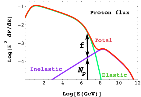
Figure 9: Elastic and inelastic contributions to the proton source spectrum. The vertical scale is $E^{2}\,dF/dE$.

Notice in Fig. 9 the different shapes of the elastic and inelastic contributions, implying that the fraction of accelerated nuclei is small, as in the results of the numerical analysis of the relativistic merging of plasmas Fred .

Many salient features of the source fluxes of CRs —the pronounced knees in the individual-element spectra, the differential changes of slope, and a maximum energy for proton acceleration— survive unscathed the many tribulations transmogrifying the source spectra into the observed ones. To discuss the comparison of predictions and data we must first summarize these tribulations.

IV Tribulations of a Cosmic Ray

On its way from its source to the Earth’s upper atmosphere, a CR is influenced by the ambient magnetic fields, radiation and matter, which it encounters. Extragalactic CRs are also affected by cosmological redshift ($z$) and the dependence of their source strength on the star-formation rate as a function of ‘look-back time’. In this section we list the tribulations of CRs —which are discussed in detail in several Appendices— and we summarize the choices we make for the priors that are not very well understood either observationally or theoretically. Three types of interactions constitute a CR tribulation:

• Interactions with magnetic fields that permeate galaxies and clusters and, presumably, the IGM.

  The fluxes of CRs of Galactic origin are, below their free-escape energy, enhanced by a factor proportional to their confinement time. At higher energies they escape the Galaxy practically unhindered.

  Extragalactic CRs entering the Galaxy must overcome the effect of its exuding magnetic wind.

• Interactions with radiation, significant for CRs of extragalactic origin. The best studied one is $\pi$ photoproduction by nuclei on the cosmic microwave background radiation, the GZK effect GZK .

  Pair ($e^{+}e^{-}$) production is akin to the GZK effect.

  The photo-dissociation of extragalactic CR nuclei, mainly on the cosmic infrared background radiation, is also extremely relevant.

• Interactions with the ISM are fairly well understood for relatively low-energy CRs of Galactic origin. Their spallation gives rise to ‘secondary’ stable and unstable isotopes in the CR flux.

Of the above items, three need be discussed here:

IV.1 Magnetic confinement and escape; the ankles

The Galaxy’s MF, whose typical value is of ${\cal{O}}(5)\,\mu$G, as in Eq. (23), varies on scales ranging up to a ‘coherence length’ of ${\cal{O}}(1)$ kpc. The MF in the Galaxy’s halo is not well charted; its typical value is similar. The Larmor radius of a CR of charge $e\,Z$ and momentum $p(E)$ is:

$$R_{L}\approx 0.65\;{\rm kpc}\;{5\;\mu{\rm G}\over B}\;{p(E)\over E_{\rm ankle}(Z)}\,,$$ (40)

$$E_{\rm ankle}(Z)\equiv Z\times(3\times 10^{18}\;\rm eV).$$ (41)

A CR of energy $E\geq E_{\rm ankle}$ cannot be significantly bent in the Galaxy. For $Z=1$, Eq. (41) coincides with the ‘ankle’ in the CR flux, see Eqs. (1).

At $E\sim E_{\rm ankle}(Z)$, Galactic CR nuclei undergo a random walk process of moderate deflections on the Galactic MF domains. Their cumulative deflection angle has a Gaussian distribution, analogous to the one describing the multiple deflection of high-energy muons in matter PDG . The escapees are the CRs deflected by less than an angle of order one radian. We need a rough description of the corresponding confinement and escape probabilies, which we characterize by:

$$P_{\rm conf}=1-P_{\rm esc}=\exp\left[-\left({E\over E_{\rm ankle}(Z)}\right)^{2}\right]\,.$$ (42)

The Galactic CR flux is modulated by the momentum dependence of the CR confinement time, $\tau_{\rm conf}$, in the disk and halo of the galaxy, affecting the different species in the same way, at fixed $p/Z$. Confinement effects are not well understood Swordy ; Ptuskin , but observations of astrophysical and solar plasmas indicate that Swordy :

$$\tau_{\rm conf} \sim K\left({Z\,{\rm GeV/c}\over p}\right)^{\beta_{\rm conf}},$$ (43)

$$K \sim 2\times 10^{7}\,{\rm y,}$$ (44)

$${\beta_{\rm conf}} \sim 0.6\pm 0.1.$$ (45)

Measurements of the relative abundances of secondary CR isotopes Swordy agree with the functional form of Eq. (43). The observed ratios of unstable CR isotopes Connell result in $K$ as in Eq. (44), but the method is well known to be biased towards low-$K$ values Longair . Our theory results in a somewhat larger predicted value of $K$, as discussed in Sections V.12, VII.

The spectrum of observable CRs of Galactic origin, $dF_{\rm Gal}/dE$, is their source spectrum, $dF_{s}/dE$, modified by confinement Axford so that $dF\!\propto\!P_{\rm conf}\,\tau_{\rm conf}\,dF_{s}$, or:

$${dF_{\rm Gal}\over dE} = C(E,Z)\;{dF_{s}\over dE}\,,$$

$$C(E,Z) \equiv P_{\rm conf}{\left[{E_{\rm ankle}(Z)\over p(E)}\right]}^{\beta_{\rm conf}}\,,$$ (46)

with $E_{L}$ and $P_{\rm conf}$ as in Eqs. (41, 42). Note that $C(E,Z)$ does not depend on the magnitude of the factor $K$ in Eq. (44).

IV.2 CR penetration into the Galaxy

In a steady-state situation, the CR flux escaping a galaxy has the energy dependence of the source flux, not the confinement-modified flux. In our CR theory, the extragalactic flux arriving to our Galaxy is simply the CR flux exiting other galaxies, modified by the tribulations of an intergalactic journey. How do these extragalactic CRs penetrate our Galaxy?

The penetration of Galactic CRs into the solar system is hindered by the ‘wind’ of solar CRs and MFs. Analogously, we proceed to argue, the penetration of extragalactic CRs into the Galaxy is hindered by the ‘wind’ of Galactic CRs and MFs. The Galaxy certainly exudes a wind of CRs: in a steady state the outgoing Galactic flux is that of the sum of Galactic sources. The question is whether the Galaxy also has an accompanying MF ‘wind’.

The Galactic CR- and MF-energy densities are known to be approximately coincident, a strong hint of an intimate relationship. In the CB model CRs are the dominant source of MFs in galaxies, clusters and the IGM (this is a tenable statement for two reasons: CR sources are kiloparsecs-long CB trajectories, as opposed to SN shells in star-formation regions, and the Galactic CR luminosity is almost one order of magnitude bigger than in the conventional view). For all these systems, the simple hypothesis of rough energy–density equipartition between CRs and MFs results in correct predictions for the intensity of the latter DDMF .

If the interaction between CRs and the ambient medium results in turbulent currents whose MFs end up storing some 50% of the energy density, we expect a large fraction of the momentum of CRs to be transferred to the MFs. This would imply the existence of a hefty Galactic MF wind. The expanding shells of SNe —and the superbubbles that ensembles of SNe generate— should also carry in their motion a Galactic MF wind.

Knowing little about the magnetic wind of the Galaxy, we cannot ascertain the probability $P_{\rm pen}(E,Z)$ that an extragalactic CR penetrates it. The flux of such CRs at the Sun’s location is renormalized by a factor $C^{\prime}(E,Z)\propto P_{\rm pen}\,\tau_{\rm conf}$, the extragalactic source analogue to $C(E,Z)$ in Eq. (46). In the absence of a wind the Galaxy would act as a diffusive magnetic ‘trap’ and, for a steady-state external flux, $P_{\rm pen}=1$. At energies above the ankle, $P_{\rm pen}$ and $C^{\prime}$ must be close to unity. At smaller energies $P_{\rm pen}$ must decrease in a manner reminiscent of the quenching of low-energy CRs by the Sun’s wind.

We have faced our ignorance on $C^{\prime}$ by trying very many different ansatzes. The features of the source spectrum (slopes, knees, ankle) are very ‘robust’ and survive unscathed the choice of a reasonable $C^{\prime}$. This is true even for the extreme ‘no-wind’ possibility: $P_{\rm pen}=1$ at all energies. However, the overall description of the data is much more satisfactory if $P_{\rm pen}<1$ below the ankle or, at least, below the knees. To illustrate this, we shall report results for two very different cases:

$${\rm(a)}\;\;C^{\prime}(E,Z) = 1$$ (47)

$${\rm(b)}\;\;C^{\prime}(E,Z) = {\left[{E_{\rm ankle}(Z)\over p(E)}\right]}^{-{\beta_{\rm conf}}}\;\;{\rm for}\;\;E<E_{\rm ankle}(Z)$$ (48)

$$= 1\;\;\;\;\;\;\;\;\;\;\;\;\;\;\;\;\;\;{\rm for}\;\;E>E_{\rm ankle}(Z).$$

Case (a) corresponds to a Galactic wind that quenches the entrance of extragalactic CRs by as much as the Galactic confinement enhances their flux, once they are in. Case (b), with ${\beta_{\rm conf}}$ as in Eq. (45), corresponds to a wind that is ‘twice as repellent’ as in case (a).

IV.3 Photo-dissociation

At energies higher than a few $10^{8}$ GeV, CR nuclei of extragalactic origin interact with the cosmic background radiation (CBR) and are photo-dissociated: one or a few nucleons per collision are stripped off. The important CBR wavelength domain extends from the ultraviolet to the far infrared, corresponding to centre-of-mass energies at which the giant dipole resonance lies. Computing the effects of photo-dissociation for a given CR source spectrum and composition, given present and past radiation densities, and given cross sections and lifetimes for parent and daughter nuclei, would be straightforward but extremely lengthy. For our current purposes it suffices to estimate the effect, which we do in Appendix B.8, summarized below.

Independent of atomic number, the approximate energy at which the mean photo-dissociation time of a nucleus travelling in the current CBR coincides with the age of the Universe is:

$$E_{\rm PhD}\simeq 7\times 10^{17}\;\,\rm eV,$$ (49)

The photo-dissociation effect on the extragalactic CR flux of (arrival) energy $E$ and (departure) atomic weight $A$ is well approximated by an attenuation factor:

$$A_{\rm PhD}(E,A)\approx{1\over\sqrt{1+[3.15\,E/(n(A)\,E_{\rm PhD})]^{2}}},$$ (50)

where $n(A)$ is an estimate of the average number of successive photo-dissociations required to reduce to $A/2$ the largest fragment of an original nucleus $A$.

IV.4 The processed fluxes

The Galactic and extragalactic fluxes at the Earth’s location are affected by the tribulations we just discussed. To illustrate this point we have split the proton and Fe fluxes of Fig. 3b into their Galactic and extragalactic contributions, and we report the result in Fig. 10. The cutoffs in the Galactic fluxes are due to CR escape, parametrized as in Eq. (46). The extragalactic fluxes are suppressed below the ankle by the Galactic penetrability effect of Eq. (47) or (48) and redshifted as discussed in Appendix B.2. The high-energy flux of extragalactic Fe is attenuated by photo-dissociation, parametrized by Eq. (50). The ultra-high energy proton flux is almost exclusively extragalactic in origin. Its shape at the highest energies is governed by the acceleration end-point of Eq. (39), the GZK cutoff of Eq. (100) and the pair-production suppression of Eq. (102).

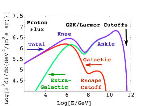
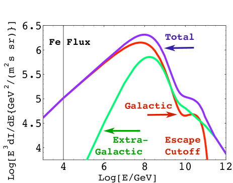
Figure 10: Features of the CR spectra for protons and Fe.

V Detailed CB-model Results

V.1 The index below the knee

The elastic contribution to the CR flux dominates below the knee, as can be seen in Fig. 9. For a large range of energies ($\sim$ ten to a million times $A\,m_{p}\,c^{2}$), this source flux is very well approximated by a power law:

$${dF_{\rm elast}\over d\gamma_{{}_{\rm CR}}}\propto\gamma_{{}_{\rm CR}}^{-\beta_{s}}.$$ (51)

The value of $\beta_{s}$ can be trivially extracted from Eq. (33). It is:

$$\beta_{s}={13\over 6}\approx 2.17.$$ (52)

The observed spectrum should be steeper, in accordance with the Galactic confinement effect of Eq. (3). The predicted index is:

$$\beta_{\rm th}=\beta_{s}+{\beta_{\rm conf}}\approx 2.77\pm 0.10,$$ (53)

in agreement with the observed value, $2.73\pm 0.03$ for protons, reported in Eq. (2); or $\sim\!2.7$ for the all-particle flux, as in Eq. (1). Above the knee and over the range, illustrated in Fig. 9, in which the inelastic contribution $dF_{\rm inel}/d\gamma_{{}_{\rm CR}}$ is well described by a power law, $\gamma_{{}_{\rm CR}}^{-\beta_{s}^{\prime}}$, its slope is steeper than that in Eq. (51): $\beta_{s}^{\prime}\approx\beta_{s}+0.3$.

The prediction of the spectral index is gratifying: simple, analytical, and almost exclusively based on trivial kinematics. It is, moreover, very insensitive to many assumptions, e.g. any non-singular non-isotropic angular distribution of particles elastically scattered by the CB in its rest system gives the same result for $\beta_{s}$ as the isotropic distribution we used here.

V.2 Relative abundances

It is customary to present results on the composition of CRs at a fixed energy per nucleus $E_{{}_{A}}=1$ TeV, as opposed to a fixed LF. This chosen energy is relativistic ($E_{{}_{A}}\simeq p_{{}_{A}}$), it is below the corresponding knees for all $A$, and it is in the domain wherein the source fluxes are dominantly elastic and are very well approximated by the power-law in Eq. (51), with the index $\beta_{s}$ of Eq. (52). Up to a common species-independent factor, then:

$${dF_{\rm source}\over d\gamma_{{}_{\rm CR}}}\propto n_{{}_{A}}\,\left({A\over Z}\right)^{\beta_{\rm conf}}\;\gamma_{{}_{\rm CR}}^{-\beta_{s}},$$ (54)

where we have taken into account the species dependence of the source flux, as in Eq. (33). Change variables ($E_{{}_{A}}\!\propto\!A\,\gamma$) in Eq. (54) and modify the result by the multiplicative confinement factor, $(Z/E)^{\beta_{\rm conf}}$, of Eq. (43) to obtain the prediction for the observed fluxes:

$${dF_{\rm obs}\over dE_{{}_{A}}}\propto\bar{n}_{{}_{A}}\,A^{\beta_{\rm th}-1}\,E_{{}_{A}}^{-\beta_{\rm th}},\,\,\,\,\,\,\,\,\beta_{\rm th}-1\sim 1.77,$$ (55)

with $\bar{n}_{{}_{A}}$ an average ISM nuclear abundance and $\beta_{\rm th}$ from Eq. (53). At fixed energy the predictions for the CR abundances $X_{{}_{\rm CR}}$ relative to protons are:

$$X_{{}_{\rm CR}}(A) \approx X_{\rm amb}(A)\;A^{1.77},$$

$$X_{\rm amb}(A) \equiv {\bar{n}_{{}_{A}}/\bar{n}_{p}},$$ (56)

where $X_{\rm amb}$ are the ambient ‘target’ abundances relative to hydrogen.

Cannonballs produce CRs while travelling in the large ‘metallicity’ environments of a SN-rich domain and the enclosing superbubble (SB). Let $X_{{}_{\rm SB}}$ be the abundances in these domains, relative to H. Only late in their voyage do CBs reach regions wherein the relative abundances of the ISM are solar-like, $X_{\rm amb}\!\simeq\!X_{\odot}$. For He the observations yield $X_{{}_{\rm SB}}\!\simeq\!X_{\odot}$. For the intermediate elements ranging from C to Ne, $X_{{}_{\rm SB}}\!\simeq\!2\,X_{\odot}$ HL . The abundances of heavier metals in SBs are poorly known. They should be close to those of old SNRs, also not well measured. One exception is SNR W49B, recently observed with XMM-newton Miceli . The best-fitted spectral parameters have resulted in $X_{{}_{\rm SNR}}/X_{\odot}$ values, $3.3\pm 0.2$ for Si, 3.7 +0.1/$-$0.2 for S, 4.2 +0.3/$-$0.4 for Ar, $6.4\pm 0.5$ for Ca, 6 +0.1/$-$0.2 for Fe and 10 +4/$-$1 for Ni. We use these values in the predictions of Eq. (55), reported in Fig. 11 and Table 2, even though the mean abundances in SBs may differ from those measured in a given SNR.

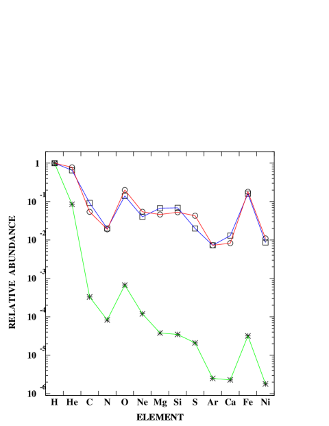
Figure 11: The relative abundances of primary CR nuclei, from H to Ni around 1 TeV WBM . The stars (joined by green lines) are solar-ISM abundances GS . The circles (joined in red) are the predictions, with input superbubble abundances. The squares (joined in black) are the CR observations.

The results of Fig. 11 are for the most abundant, dominantly primary CRs. We have suppressed the error bars of the input $X_{{}_{\rm SB}}$ values: even the size of the errors is debatable. Yet, the results are satisfactory. In spite of its simplicity, Eq. (55) snugly reproduces the large enhancements in the heavy CR abundances relative to hydrogen, with respect to solar or SB abundances.

In Table 2 we report in detail the abundances of the primary and secondary (mainly odd-$Z$) elements. The predictions of Eq. (55) are slight overestimates of the CR observations for intermediate and heavier primaries. For the CR secondaries, the predictions are always underestimates. When elements are added in groups of primaries and their most abundant secondaries, the agreement between theory and observation is even better. All this is to be expected: we have not considered the nuclear spallations depleting primaries and making secondaries.

Table 2: Solar abundances and CR abundances at 1 TeV, both relative to hydrogen.

	Z	$X_{\odot}$	$X_{{}_{\rm CR}}$	$A^{1.73}\,X_{{}_{\rm SB}}$
H	1	1	1	1
He	2	$7.5\times 10^{-2}$	$6.5\times 10^{-1}$	$8.2\times 10^{-1}$
C	6	$3.3\times 10^{-4}$	$9.2\times 10^{-2}$	$4.9\times 10^{-2}$
N	7	$8.3\times 10^{-5}$	$2.0\times 10^{-2}$	$1.6\times 10^{-2}$
O	8	$6.7\times 10^{-4}$	$1.4\times 10^{-1}$	$1.6\times 10^{-1}$
Ne	10	$1.2\times 10^{-4}$	$3.8\times 10^{-2}$	$4.3\times 10^{-2}$
C–Ne			$2.9\times 10^{-1}$	$2.7\times 10^{-1}$
Na	11	$2.2\times 10^{-6}$	$6.5\times 10^{-3}$	$1.7\times 10^{-3}$
Mg	12	$3.8\times 10^{-5}$	$6.7\times 10^{-2}$	$3.2\times 10^{-2}$
Al	13	$3.0\times 10^{-6}$	$1.0\times 10^{-2}$	$3.1\times 10^{-3}$
Si	14	$3.5\times 10^{-5}$	$6.9\times 10^{-2}$	$3.7\times 10^{-2}$
P	15	$2.8\times 10^{-7}$	$2.3\times 10^{-3}$	$3.7\times 10^{-4}$
S	16	$2.1\times 10^{-5}$	$2.0\times 10^{-2}$	$3.2\times 10^{-2}$
Cl	17	$3.2\times 10^{-7}$	$2.6\times 10^{-3}$	$6.0\times 10^{-4}$
Ar	18	$2.5\times 10^{-6}$	$7.3\times 10^{-3}$	$6.2\times 10^{-3}$
K	19	$1.3\times 10^{-7}$	$4.7\times 10^{-3}$	$3.8\times 10^{-4}$
Ca	20	$2.3\times 10^{-6}$	$1.3\times 10^{-2}$	$8.7\times 10^{-3}$
Na–Ca			$2.0\times 10^{-1}$	$1.3\times 10^{-1}$
Sc	21	$1.4\times 10^{-9}$	$2.6\times 10^{-3}$	$6.5\times 10^{-6}$
Ti	22	$1.0\times 10^{-7}$	$9.8\times 10^{-3}$	$5.2\times 10^{-4}$
V	23	$1.0\times 10^{-8}$	$5.5\times 10^{-3}$	$5.8\times 10^{-5}$
Cr	24	$4.7\times 10^{-7}$	$1.2\times 10^{-2}$	$2.8\times 10^{-3}$
Mn	25	$2.5\times 10^{-7}$	$1.2\times 10^{-2}$	$1.6\times 10^{-3}$
Fe	26	$3.2\times 10^{-5}$	$1.6\times 10^{-1}$	$2.0\times 10^{-1}$
Co	27	$8.3\times 10^{-8}$	$6.5\times 10^{-4}$	$6.2\times 10^{-4}$
Ni	28	$1.8\times 10^{-6}$	$8.6\times 10^{-3}$	$2.0\times 10^{-2}$
Sc–Ni			$2.1\times 10^{-1}$	$2.2\times 10^{-1}$

V.3 Composition dependence of the spectral slopes

At each local value of its decelerating LF, $\gamma$, a CB exudes elastically scattered CRs with LFs $\gamma_{{}_{A}}$ in the range $1\leq\gamma_{{}_{A}}\leq 2\,\gamma^{2}$, as well as internally pre-accelerated CRs in the range $1\leq\gamma_{{}_{A}}\leq 2\,b\,\gamma^{2}$; see Section III.1. The higher-energy CRs must have been gathered by a CB from the ISM when $\gamma$ is close to $\gamma_{0}$ and the CB is close to its place of origin, where the abundance of the elements is that of a star-forming region or its surrounding SB. The lower-energy CRs are generated all along the CB’s trajectory and pile-up from its low-$\gamma$ end, a point at which a CB is typically travelling in a ‘normal’ ISM, with a composition close to that of the solar neighbourhood. This complicated effect may be approximated by a composition-dependence of the spectral slopes, $\beta_{{}_{A}}$, of the flux of the different nuclei.

To illustrate this point, consider the CR flux below the knee, dominated by elastically scattered CRs. Adopt an extreme simplifying ansatz: that CRs with $\gamma\sim 2\,\gamma_{0}^{2}$ are accelerated within SBs, whereas CRs with $\gamma\sim 1$ are accelerated in the ISM further away from the SBs. Since the abundance of Fe nuclei in the SB is $\sim 6$ times larger than their abundance in the average ISM, the flux of CR Fe nuclei with $\gamma\sim 2\,\gamma_{0}^{2}$ is enhanced by a factor $\sim 6$ relative to their flux at $\gamma\sim 1$. This is equivalent to a change $\Delta\beta_{\rm Fe}$ in the slope of the CR Fe flux which satisfies

$$[2\,\times\gamma_{0}^{2}]^{\Delta\beta_{\rm Fe}}\approx[3\times 10^{6}]^{\Delta\beta_{\rm Fe}}=6,$$ (57)

or $\Delta\beta_{\rm Fe}\approx 0.12$. The predicted slope of the Fe spectrum below the knee is then $\beta_{\rm Fe}=\beta_{\rm th}-\Delta\beta_{\rm Fe}=2.65$, with $\beta_{\rm th}$ as in Eq. (53), in good agreement with the observed $\beta_{\rm Fe}=2.60\pm 0.10$ WBM .

The above exercise can be redone for the rest of the elements, with the result that, to a good approximation, $\beta_{{}_{A}}\simeq\beta_{\rm th}-0.03\,\ln(A)$ DAD . The predicted and observed slopes below the knees are shown in Fig. 12.

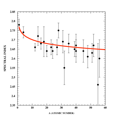
Figure 12: A rough prediction of the $A$-dependence of the spectral indices around 1 TeV, shown for some of the most abundant primary elements WBM . The spectral slopes of H and He are those measured by AMS AMS .

V.4 The normalization of the extragalactic flux

The cleanest place of choice to discuss the normalization of the CR spectrum is at —or slightly above— the ankle. At such an energy CRs are extragalactic and their spectrum is insensitive to Galactic MFs and winds, to the GZK and CB-acceleration cutoffs of Eqs. (100, 39), to the effects of photo-dissociation above the energy of Eq. (49), to the distribution of LFs of Eq. (6), to the ‘elastic-scattering’ contributions ending at the much lower energies of Eq. (34), and to the detailed composition of CRs, for only H is abundant at that energy.

Let $\epsilon_{{}_{\rm U}}$ be the energy-integrated, average current energy flux of CRs in intergalactic space, accumulated over look-back time $t(z)$. Up to the highest energies —at which effects such as the GZK cutoff are relevant— there is nearly no energy loss except for the redshift effect, and:

$$\epsilon_{{}_{\rm U}}={c\over 4\,\pi}\,R_{\rm SN}{\rm[U]}\int dz\,{dt\over dz}\,{E[{\rm jets}]\over 1+z}\,{R_{\rm SF}(z)\over R_{\rm SF}(0)},$$ (58)

where $dt/dz$ is the time to redshift relation specified in Appendix B.2; $R_{\rm SN}\rm{[U]}$ is the average current SN rate per unit universal volume, given by Eq. (97); $E[{\rm jets}]$, as in Eq. (18), is the average jet energy per SN; and $R_{\rm SF}(z)$ is the star-formation rate reviewed in Appendix B.4.

The extragalactic flux has the energy distribution of Eq. (93). Its normalization is specified by the constraint:

$$\int_{E_{\rm min}}E\;{dF{\rm[EG]}\over dE}=\epsilon_{{}_{\rm U}},$$ (59)

which allows us to compute $dF{\rm[EG]}/dE$ at any energy, using the observed (or fitted) CR flux and the adopted correction for Galactic confinement, Eq. (46). The result is proportional to $E_{\rm min}^{-0.2}$: insensitive to $E_{\rm min}$. For $E_{\rm min}=1$ GeV and our predicted indices, the result at $E=E$[ankle] is:

$$E^{3}\,{dF{\rm[EG]}\over dE}\Big{|}_{E{\rm[ankle]}}\sim 10^{24}\;\rm eV^{2}\,m^{-2}\,s^{-1}\,sr^{-1}.$$ (60)

An extrapolation from $E\sim E_{\rm min}$ —where most of the CR flux and energy reside— to $E=E$[ankle] would seem to be inordinately sensitive to the adopted spectral indices. But the theory fits the data over this large domain! The result of Eq. (60) is a gratifying number, as we proceed to discuss.

V.5 Questions of presentation

We shall see in the next Subsection that the result of Eq. (60) allows us to predict the shape and normalization of the UHECR flux. The prediction of the normalization has an uncertainty that reflects the combined uncertainties of various inputs, such as the fraction of core-collapse SNe that generates GRBs (to which we dedicate Appendix D.3), the error in the value of the prior $E[{\rm jets}]$, the uncertainty in the distribution of $\gamma_{0}$ values and in the star formation rate $R_{\rm SF}(z)$ at $z\sim 1$ to 2, the redshifts dominantly contributing to the integral in Eq. (58). The nominal error on each of these quantities is a factor of 2 or more and hard to ascertain with precision. The combined error in the prediction is larger than that of the normalization of the UHECR flux (a statistical error of a factor of about 2, if we restrict ourselves to measurements made with a single technique, such as the fluorescence of the CR showers).

We could choose to present our prediction for the UHECR flux as a wide band reflecting the uncertainty in the normalization. Alternatively, we could use the CR data to constrain the priors to a multidimensional domain narrower than the prior one. We opt for a third possibility: to choose a normalization —within its predicted domain— that compares well with the UHECR observations, making the result for the spectrum ‘look better’. We make the same choice elsewhere, e.g. the CR abundances relative to protons are correctly predicted within a factor of order 2, yet, we shall fix the overall normalization of the corresponding spectra to compare well with the normalization of the observations. None of the above affects the results for the shapes of the spectra.

In all of our results, a comprehensive best fit of all parameters and priors may make the comparison with data ‘look even better’. Such an effort would be premature: the observations of the CR flux are still a fluid issue, our detailed choices do not all indisputably follow from first principles.

We choose to present our results for the CR spectra in order of descending energy.

V.6 The UHECR spectrum

Our prediction for the UHECR all-particle spectrum is shown in Fig. 13. At $E=E$[ankle] the extragalactic contribution of Eq. (60) is about 1/2 of the observations reported in the figure. Its normalization, at this energy or above it, is approximate but ‘absolute’, in the sense discussed in the previous subsection. The shape of the flux above the ankle is entirely predicted; it is the shape of the redshifted flux of Eq. (93).

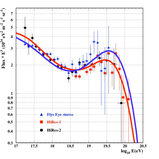
Figure 13: Predicted and observed HIRES1 UHECR spectrum. The vertical scale is $E^{3}\,dF/dE$. The normalization and shape of the spectrum above the ankle do not involve any fit parameters, only choices of priors within their predetermined domains.

The two curves of Fig. 13 correspond to the two choices of penetrability of extragalactic CRs to the Galaxy: the blue curve rising higher uses Eq. (48) with ${\beta_{\rm conf}}=0.55$, the red curve uses Eq. (48) with ${\beta_{\rm conf}}=0.5$. The curves have slightly different central values and widths of the $\gamma_{0}$ distributions of Eq. (6), both within the corresponding prior domains: $\bar{\gamma}_{0}=1200$ (1300), $w=0.4$ (0.5) for the blue (red) lines. In the two curves in Fig. 13 the shape of the high-energy end-point and the height of the hump reflect not only the GZK cutoff of Eq. (100), but also the acceleration-cutoff energy for protons, which has been properly smeared with the corresponding $\gamma_{0}$ distribution.

V.7 The ankle region and the flux normalization

Above the ankle, the CR flux is dominated by protons of extragalactic origin belonging to the high-energy ‘inelastic’ part of their source spectrum. The overall normalization of this spectrum is the quantity $N_{p}$ illustrated in Fig. 9, whose approximate predicted value is implied by Eq. (60). The refinement of this prediction to agree with the data shown in Fig. 13 narrows down the value of $N_{p}$ to better than a factor of 2.

To fit the flux of protons below the proton knee, we will have to fix our only free parameter: the elastic-to-inelastic ratio $f$ of Fig. 9. In our theory, $f$ is species-independent and the relative CR abundances are predicted. Hence, once $N_{p}$ and $f$ are fixed, the spectrum of CRs of all nuclear species is fixed. In particular, the Fe flux is predicted. The knee of the Fe flux dominates the all-particle spectrum just below the ankle. At the ankle, its contribution to the total flux of Fig. 13 is about 50%. So, the ankle is indeed the energy above which the extragalactic flux takes over Cocconi .

The ankle may be defined as the energy at which CR protons are no longer expected to be confined to the Galaxy, as in Eqs. (40, 41). The ankle happens to occur at this energy, but it is not the end-point of a dominantly Galactic proton flux. It is, however, the starting point of a dominantly extragalactic proton flux. This is not the only ‘ankle coincidence’. The shape of the CR flux, at the ankle and just above it, is partly due to the effect of $e^{+}e^{-}$ production on the extragalactic proton flux, illustrated in Fig. 31. The energy at which this attenuating effect is maximal coincides with $E_{\rm ankle}(Z\!=\!1)$, but has nothing to do with CR confinement in the Galaxy. In galaxies unlike ours these coincidences need not take place. This prediction may be particularly difficult to test.

V.8 The all-particle spectrum

Our results for the all-particle spectrum are shown in Fig. 14. The normalization of this plot is fixed by the parameter $f$ (fit to proton data at the knee), the combination of priors $N_{p}$ (adjusted within its pre-established domain) and the predicted relative abundances of the CR elements. The shape of the theoretical curves is thereby fixed. Naturally, their tilt and the sharpness of the ankle are sensitive to the chosen value of ${\beta_{\rm conf}}$, which appears in the exponential of an energy dependence that extends over many decades. The colour-coded lines correspond to the same choices as in Section V.6 and Fig. 13.

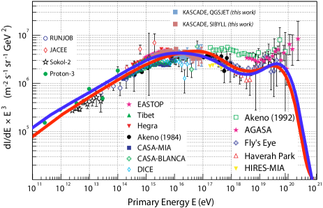
Figure 14: Fitted and observed all-particle CR spectrum. The vertical scale is $E^{3}\,dF/dE$. Some of the UHECR data in this figure disagree with the ones in Fig. 13. The color-coded lines correspond to the same choices as in Section V.6 and Fig. 13.

V.9 The knee region

There are recent data from the KASKADE collaboration attempting to disentangle the spectra of individual elements or groups in the knee region. The data are preliminary in that their dependence on the Monte Carlo programs used to simulate hadronic showers is still unsatisfactorily large. Our predictions for the spectra of H, He and Fe are shown in Fig. 15. The red and blue lines correspond to the same choices as in Section V.6 and Fig. 13. The green line in the proton entry has $w=0.8$ for the width of the $\gamma_{0}$ distribution, as in Fig. 5, the red and green lines correspond to distributions about $2\sigma$ and $3\sigma$ wider and, within the large systematic uncertainties of the data, seem to be ‘better’.

At the highest energies, the blue line in the H figure curves up, as the corresponding inelastic contribution begins to dominate. Since the elastic and accelerated distributions are additive, the theory predicts not only a knee —at the point where the elastic contribution is rapidly cut off— but rather a ‘kneecap’, ending at the point at which the inelastic contribution takes over. This is more clearly visible in Fig. 9.

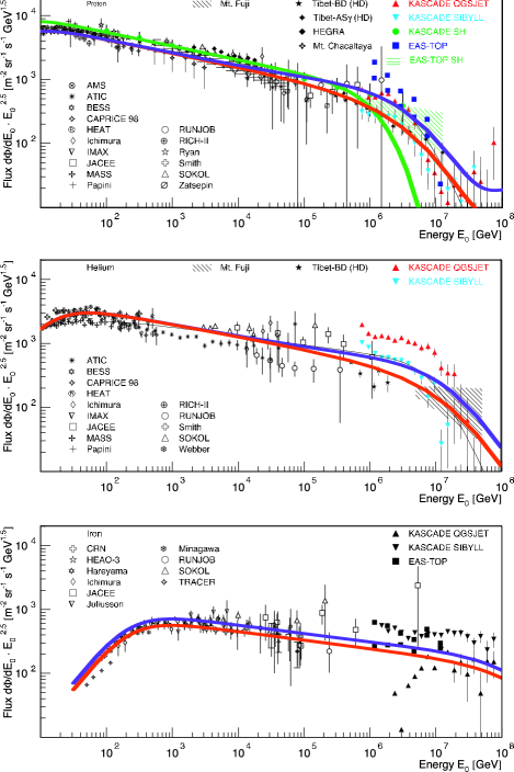
Figure 15: Measurements of individual-element CR spectra in the ‘knee’ region Hoer . The vertical scales are $E^{2.5}\,dF/dE$. Top: protons; Middle: $\alpha$ particles; Bottom: iron nuclei. The colour-coded lines correspond to the same choices as in Section V.6 and Fig. 13. The green line in the proton entry has $w=0.8$ for the width of the $\gamma_{0}$ distribution, as in Fig. 5. The compilation of data was kindly provided to us by K.H. Kampert.

V.10 The low-energy spectra

The lower the energy, the easier the sieving of CRs into individual elements and their isotopes. In Fig. 16 we show the weighted spectra $E_{k}^{2.5}\,dF/d\,E_{k}$ of protons and $\alpha$ particles, as functions of $E_{k}$, the kinetic energy per nucleon. The figure shows data taken at various times in the 11-year solar cycle. The most intense fluxes correspond to data taken close to a solar-minimum time. The theoretical curves do not include an attempt to model the effects of the solar wind. They should agree best with the solar-minimum data, as they do, particularly for protons.

The theoretical spectra, dominated by the elastic contribution to the CR spectrum, are given by Eq. (33). The data in Fig. 16 are well below the elastic cutoff at $\gamma_{{}_{\rm CR}}\simeq 2\,\gamma_{0}^{2}$, meaning that the result is independent of the chosen $\gamma_{0}$ distribution. Thus, the shape of the theoretical source spectra is, in this energy domain, parameter-free. At the lowest energies shown in Fig. 16, the differences between the exact result of Eq. (32) and its non-relativistic approximation of Eq. (33) are at the 20% level. At these energies CRs are confined for very long times and their interactions with the ISM —which we have not corrected for— result in similar corrections. Uncertainties of the same order are also introduced by our neglect of solar-neighbourhood effects. The results of Fig. 16 may look better than they should.

The curves in Fig. 16 are sensitive to the chosen value of the confinement exponent ${\beta_{\rm conf}}$ of Eq. (3), which governs the overall ‘tilt’ of the curves. In this figure we have chosen ${\beta_{\rm conf}}=0.6$, reflecting a general tendency of the data to be better described by slightly higher values of ${\beta_{\rm conf}}$ at low energies (recall that the results for the all-particle spectrum and the knee region have either ${\beta_{\rm conf}}=0.5$ or ${\beta_{\rm conf}}=0.55$). We could have chosen to present all results with an input ${\beta_{\rm conf}}$ reflecting the errors in this prior; see Eq. (3). To some extent this is purely a question of cosmetics in the presentation; one reason is that the addition of best fits to the data on individual elements differs from a best fit to the all-particle spectrum!

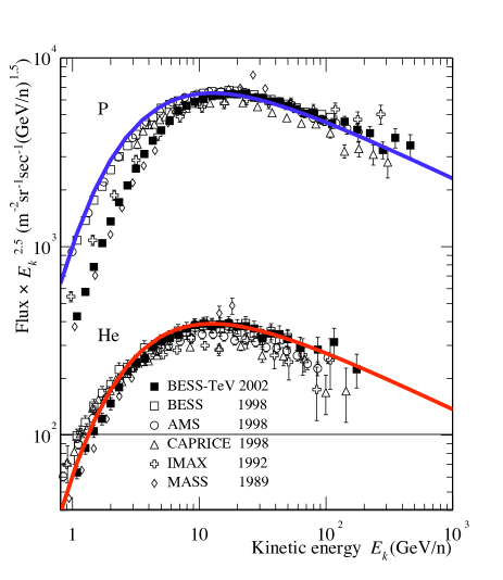
Figure 16: The very low energy fluxes of protons and $\alpha$ particles at various times in a solar cycle. The 1998 data are close to solar-minimum time.

V.11 Rough measures of CR composition

The evolution of the CR composition as a function of energy is often presented in terms of two quantities: the mean logarithmic atomic weight $\langle\ln A\rangle$ and the depth into the atmosphere of the ‘maximum’ of the CR-generated particle shower, $X_{\rm max}$. The predicted $\langle\ln A(E)\rangle$ is compared with relatively low-energy data in Fig. 17. The predicted $X_{\rm max}(E)$, constructed with a simplified method described by Wijmans Wigmans , is shown in Fig. 18.

The predicted $\langle\ln A(E)\rangle$ at all energies, shown in Fig. 19, shows how at very high energies the flux is once more Fe-dominated: lighter elements have reached their acceleration and Galactic-escape cutoffs. Naturally, this prediction is very sensitive to the assumed details of Galactic escape and extragalactic photo-dissociation.

      

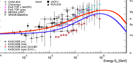
Figure 17: Mean logarithmic mass of high energy CRs. Data points were compiled by Hoerandel Hoer from experiments measuring electrons, muons, and hadrons at ground level. The colour-coded lines correspond to the same choices as in Section V.6 and Fig. 13. The compilation of data was kindly provided to us by K.H. Kampert.

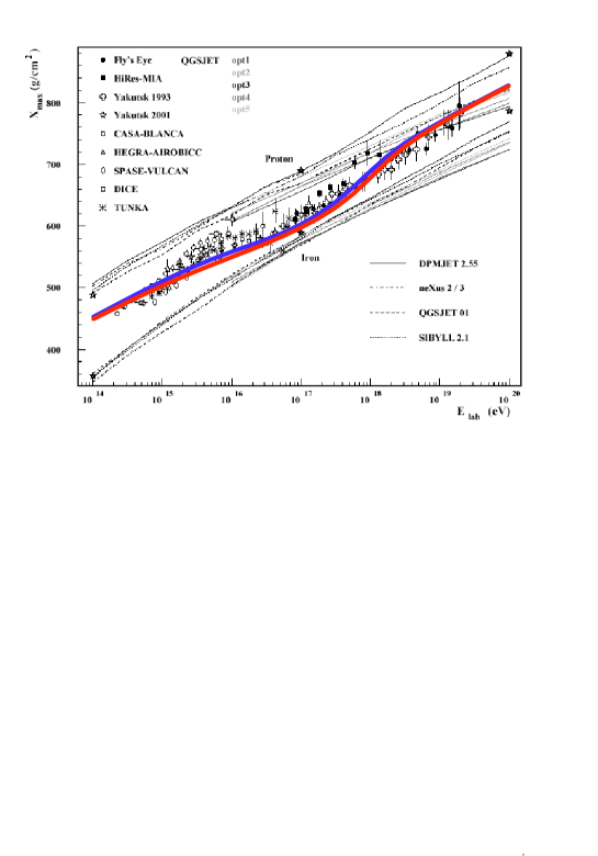
Figure 18: The depth of shower maximum as a function of energy. The data are from a compilation in Ref. ZKP . The color-coded lines correspond to the same choices as in Section V.6 and Fig. (13).

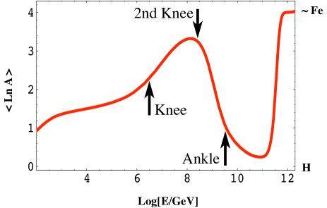
Figure 19: The prediction for $\langle\ln A(E)\rangle$ at all energies.

V.12 The confinement time and volume

The adopted form of the confinement-time function $\tau_{\rm conf}(E)$ of Eq. (45) implies a constraint that may be re-expressed as a prediction of the coefficient $K$ in Eq. (45). Similarly, the CB-model value of the Milky-Way’s luminosity, Eq. (21), and its expression Eq. (19) in terms of the confinement volume, $V_{\rm CR}$, can be used to predict the value of the latter.

The largest coherent magnetic-field domains in the Galaxy have sizes of ${\cal{O}}(1)$ kpc Beck . The light-travel time in such a domain must approximately correspond to the confinement time for protons of energy $E=E(\rm ankle)$. With this constraint, using Eq. (45) for $Z=1$, we can make a very rough estimate of the coefficient $K$ in the expression for $\tau_{\rm conf}$. The result is $K\sim 2\times 10^{8}\,{\rm y}$, one order of magnitude larger than the value quoted in Eq. (44), which is also fairly uncertain DDGBR and is known to be an underestimate Longair . In discussing the spectrum of CR electrons in Section VII we shall see that in our theory there is another way of estimating $K$, whose result is also $K\sim 2\times 10^{8}\,{\rm y}$.

Approximate Eq. (19) with an assumed fairly uniform CR flux in the Galaxy, the expectation in our theory, thereby defining an effective confinement volume:

$$V_{{}_{\rm CR}}\sim L_{p}\;\left({4\pi\over c}\,\int{dE\over\tau_{\rm conf}}\,E\,{dF_{p}\over dE}\right)^{-1}.$$ (61)

For the predicted luminosity of the Galaxy, Eq. (21), and the observed proton luminosity, the result is $V_{{}_{\rm CR}}\!\approx\!1.6\!\times\!10^{69}$ cm³. This is in agreement with the volume, $V_{{}_{\rm CR}}\!=\!(\pi)^{3/2}\,\rho_{e}^{2}\,h_{e}\!=\!1.6\times 10^{69}\,{\rm cm^{3}}$, of a Galactic CR halo of 35 kpc radius and 8 kpc height above the disk, inferred from our study of the GBR DDGBR ; DDDGBR2 , summarized in Section VIII. This volume is consistent with our estimate of the confinement time of Galactic CRs. The volume $V_{{}_{\rm CR}}\!\approx\!6.6\!\times\!10^{68}$ cm³, obtained by Strong et al. Str4 in an elaborate leaky box model of the Galaxy, is smaller by a factor $\approx 2.5$ than our estimate, reflecting the shorter confinement time of CRs in leaky box models, and the higher value adopted in Str4 for the extragalactic GBR.

VI Discussion

We have presented a specific version of the theory, implying several concrete assumptions and choices. In this Section we further discuss these choices, as well as the ‘robustness’ of the predictions, i.e. their relative independence of our chosen inputs. The conclusion is that all of the general properties of the results, listed in our Conclusions, are robust.

VI.1 The CB-model priors

VI.1.1 The CR luminosity

We have argued in Sections II.8, V.6 and V.8 that our predicted CR luminosity agrees with observations. This means that no other sources of non-solar CRs need be invoked. Yet, the agreement of theory and observations is ‘within large errors’. The question arises of whether or not other sources of CRs may be relevant.

We devote Appendix F to the discussion of the relative CR luminosity of other sources: pulsars, soft $\gamma$-ray repeaters, neutron-star mergers, and micro-quasars. Our conclusion is that their putative contribution is in every case negligible. We dedicate Section VIII.3 to the contibution of AGNs to the GBR, which is very relevant, in our theory, to their putative contribution to UHECRs, discussed in Sections IX and X.4.

The only remaining conventional candidate for a source of CRs is the non-relativistic expanding shells of SNe. Literally thousands of papers have been written on this subject. Many of them recognize that the theory is not supported by observations of the flux of $\gamma$-rays that nuclear CRs impinging on the local ISM would generate via $\pi^{0}$ production and subsequent decay, nor by the near-isotropy of the CR flux at our location in the solar circle, external to the domain where most massive stars (potential SNe) lie. One prominent example of a discussion of these points is the 1957 review by Philip Morrison Morrison . A much later and very incisive example is the commentary by Rainer Plaga in Plaga . Yet, having received so much attention in spite of its well-known flaws and limitations, this conventional SNR theory of relatively low-energy CRs is unlikely to be abandoned. We choose not to attempt to discuss the subject in detail, except for the important questions of the total CR luminosity, which has triggered controversy, and of recent results by the HESS and MAGIC collaborations, which have triggered great interest, and are discussed in Section X.5.

The standard result of Eq. (20) is a factor $\sim\!6$ smaller than our Eq. (21). Dogiel, Schönfelder and Strong DSS criticized our original result for the luminosity DDLum , which was somewhat larger (we used at the time a rough estimate of $E{\rm[jets]}$ based on the natal kicks of neutron stars). Their critique is phrased entirely within models in which the CRs are produced in the central realms of the Galaxy (interior to the solar circle) and diffuse to the rest of the Galaxy and its halo. The result is inapplicable to the CB model, wherein CRs are made much more uniformly: over the entire trajectories of CBs, which extend all the way to the halo and beyond, as discussed in Section II.4.

In this paper we have adopted a 1 to 1 association between GRBs and core-collapse SNe. As discussed in Appendix D.3 this is subject to ‘cosmological’ and CB-model uncertainties, both of ${\cal{O}}(2)$. Within errors, it may be that a subclass of SNe, e.g. those of Type Ib/c, is responsible for the majority of long-duration GRBs. In that case, our estimates of the CR luminosity may be correspondingly reduced.

VI.1.2 The deceleration of a CB and the index below the knee

In deriving Eqs. (7,8) we have worked in the approximation wherein the diffusive rate of escape of ISM particles from a CB is slower than their incoming rate. To study a large range of possibilities, consider the opposite extreme, in which the escape is instantaneous at all values of the CB’s LF $\gamma$. Let $a$ be the ratio between the average energy of a nucleus exiting a CB in its rest system and the energy at which the nucleus entered, so that $\langle\gamma_{\rm out}\rangle\equiv a\,\gamma$. For elastic scattering, $a=1$; for nuclei phagocytized by the CB, $a=0$; and for those Fermi-accelerated within the CB, $a\!>\!1$. Let $\bar{a}$ be the mean value in the average over these processes. Energy–momentum conservation implies a CB’s deceleration law:

$${d\gamma\over\beta^{k}\,\gamma^{k}}\simeq-{m_{p}\over M_{0}}\,{\gamma_{0}^{\bar{a}-1}}\;dn_{p}\;,\;\;\;\;\;\;k\equiv 3-\bar{a}\,,$$ (62)

and a CB’s inertial mass evolving as:

$$M=M_{0}\;\left({\beta\,\gamma\over\gamma_{0}}\right)^{2-k}.$$ (63)

For $a>0$, Eqs. (62,63), imply a slightly different deceleration law than Eqs. (7,8), and a smaller $\beta_{s}$ than that of Eq. (52). A related uncertainty is the one introduced by the adopted form of $R_{\rm CB}(\gamma)$, which affects $\beta_{s}$ via Eqs. (24), (28). We argue in detail in Appendix A that this is the right choice, and is supported by GRB X-ray AG data, but our theoretical arguments are admittedly over-simplifications of the extremely complex problem of the CB–ISM collisional process. Yet another source of uncertainty in the prediction of $\beta_{\rm th}$ relates to the fact that cosmic MFs are in rough energy equipartition with CRs, both in the Galaxy and in larger systems DDMF . The transfer of as much as 50% of their initial energy from CRs to the MFs they generate may affect the slope of the CR spectrum, if the transfer efficiency is not energy-independent. In spite of all these caveats, since the errors in the uncertainty ${\beta_{\rm conf}}$ of Eq. (3) are large, the prediction for the observed $\beta_{\rm th}$ of Eq. (53) is still quite satisfactory.

The prediction of the spectral slope of Eq. (52) is insensitive to all other details of its derivation. An example: we have assumed the re-emission of ISM particles in the CB’s rest system to be isotropic. We may have assumed the distribution to be that of scattering by a hard ball (modelling a CB’s highly magnetized surface), by a monopole (modelling an electrically charged CB) or a dipole (modelling a CB’s longest-range MF component). These distributions do not affect $\beta_{s}$, though they give slightly different shapes to the elastic flux close to the knee.

VI.1.3 Location of the Galactic CR sources

We have adopted here a version of our theory wherein the rate at which CRs exit a CB is much slower than that at which they enter it, as in our recent study of X-ray AGs DDDSwift . In previous analyses of GRB AGs AGoptical ; AGradio , as well as in our first results on CRs Florence , we studied the ‘fast’ opposite limit: the ISM particles intercepted by a CB are instantaneously scattered. The results in the two limits, for AGs and CRs, are very similar: we have no convincing way to opt for one or the other limit.

Let $\vec{r}$ be the vector position of a point in the Galaxy relative to its centre. Let $n(\vec{r})$ be the ISM density. To sketch a point, consider the rough approximation wherein SNe occur only close to the Galactic centre. In the ‘fast’ limit, the CR source is distributed in proportion to $n(\vec{r})$ times the density of CB trajectories, that is $n(\vec{r})/r^{2}$. In the extreme ‘slow’ limit DP the sources of CRs are located at the points where CBs end their voyage; a prediction of their distribution would require a very detailed modelling of the distribution $n(\vec{r})$ in the entire Galaxy.

There is yet another source of uncertainty in the precise distribution of the Galactic CR sources. The narrow conical beams of CRs produced by the decelerating CBs may propagate collectively, sweeping up the MF in front of them until the energy density in the beam becomes smaller than that of the field. Thereafter the CRs would begin to diffuse in the ambient MF as individual particles. Such a mechanism may effectively remove the source further away from the SNe firing the CBs, and contribute to the explanation of the high isotropy of Galactic CRs at all energies.

VI.1.4 Fermi acceleration within a CB

We have been very specific in choosing the Fermi-accelerated spectrum of Eq. (17). Its abrupt threshold $\Theta(\gamma_{A}-\gamma)$ may be substituted by a much smoother function describing how unlikely it may be to ‘Fermi-decelerate’ a fraction of the particles tossed around by moving MFs. Once processed through the CB-deceleration integrals in Eq. (37), no significant changes occur in the predicted CR flux, except that the ‘little knee’ shown in Fig. 9 at $E\sim 10^{8}$ GeV becomes less pronounced (depending on the specific choices of this and other priors, one may obtain smoother spectra, such as those in Fig. 3, or move the little knee to an energy at which it looks like a ‘rotula’ before the steepening at the knee). The results are even more insensitive to the abrupt Larmor cutoff $\Theta(\gamma_{\rm max}-\gamma_{A})$ of the assumed input spectrum. The prediction of the UHECR flux would only be affected if the radius of a CB, or the MF within it, were smaller than the ones of Eqs. (9), or (12), by more than one order of magnitude.

In the calculations we have presented, we used $\beta_{\rm ac}=2.2$, as in Eq. (13). This affects the slope of the accelerated flux via Eq. (37). We have also worked out the results for $\beta_{\rm ac}=2.2\pm 0.2$. For the upper value, they ‘look even better’ than the results we have presented. For the lower value they are similar, for slightly different chosen values of the confinement exponent ${\beta_{\rm conf}}$ and the width of the $\gamma_{0}$ distribution. This relative insensitivity is good news: for the mechanism accelerating particles within a CB, we have relied on ‘first-principle’ numerical analyses Fred , but so far their results are very limited in their study of the parameter space: the electron to proton mass ratio is unrealistic, the LF values are much smaller than $10^{3}$, the density contrast between the two merging plasmas is low, radiative effects (which are important for electrons) are neglected, and the merging plasmas are semi-infinite in extent (modelled with a finite transverse size and periodic boundary conditions).

On the positive side, the value of $\beta_{\rm ac}$ that we have adopted, if common —as we assume— to nuclei and electrons, is strongly supported by the observations of the “prompt” ICS-generated spectrum of GRBs DD and of the SR-generated spectrum of their AGs, discussed in some detail in Section X.1.

VI.2 The non-CB-model priors

VI.2.1 The relative abundances in the ISM

We contend that CBs accelerate the target ISM particles to CR energies, mainly during their voyage through the superbubble domains enclosing most SNe. As we discussed in Section V.2, the relative abundances in these domains are poorly known, resulting in large errors in the CR abundances predicted in Eq. (56). The errors are not large enough to invalidate the comparison between different mechanisms of CR acceleration, a simple task in the analysis of the CR composition:

In the conventional theory of CR acceleration by the non-relativistic ejecta of SNe, the CR composition directly reflects the relative abundances of the ISM, in this case the medium surrounding the SN shell. The comparison in Fig. 20 is often used to illustrate how the abundance of secondary CRs is enhanced relative to their ambient (solar or interstellar) abundances and how the abundances of the primary CRs follow the pattern of ambient abundances. The second conventional claim is not quite correct: the figure demonstrates that the statement is up to three orders of magnitude wrong in the comparison of Fe to H. Contrarywise, for $A\!=\!56$ in Eq. (56), $X_{{}_{\rm CR}}\!=\!1242\,X_{\rm amb}$. This explains the difference between Figs. 11 and 20 regarding the abundances of primaries.

Figure 20: Composition of CRs with $Z\!\leq\!28$ at 1 TeV wiebel ; pg .

VI.2.2 Confinement in and penetration into the Galaxy

In implementing the effects of Galactic MFs on the confinement of CRs we have used the results of Eqs. (43), (46), which are based on observational results for relatively low energies, and applied them up to the Galactic escape energies of Eqs. (41,46). It is quite conceivable that the confinement exponent ${\beta_{\rm conf}}$ is not a fixed number over all of this range, and we have commented on how a ${\beta_{\rm conf}}$ that slightly decreases with energy improves the presentation of the results. There is some theoretical understanding of the value of ${\beta_{\rm conf}}$. A turbulent Kraichnan spectrum of magnetic inhomogeneities yields ${\beta_{\rm conf}}=0.5$ Ptuskin , compatible with the low-energy observations, Eq. (45). But not enough is known about the MF of the Galaxy to opt for a particular spectrum of inhomogeneities, or a transition energy from one case to another.

Fits to CR data employing our fixed source spectra and a value of ${\beta_{\rm conf}}$ that slowly diminishes with energy provide very satisfactory results. Moreover, they increase the domain of acceptable possibilities for the description of Galactic penetrability by extragalactic CRs, which we have narrowed down in this paper to the choices of Eqs. (47,48). We do not report the various possibilities we have explored, given our ignorance of the detailed properties of Galactic fields and winds.

VI.2.3 Interactions with matter and radiation

The interactions of CRs with radiation and the ISM, listed in Section IV and discussed in various Appendices, are well understood. The exception is the photo-dissociation of extragalactic nuclei which, though well understood in principle, has not been studied in full detail. We have estimated it in a manner that should be sufficient for our current purposes. The main impact of a careful study would be to gain confidence in the predictions of our theory (or any other sufficiently specific theory of UHECR sources) concerning the relative abundances at very high energy.

VII Cosmic-Ray electrons

In this Section and the next, we give a simplified description of CREs and the GBR in the context of the CB model. More details can be found in Refs. DDGBR and DDDGBR2 .

Electrons and nuclei are accelerated by the ‘magnetic-racket’ CBs in the same manner. The functional form of their source spectra is therefore the same, approximately $dF_{s}/d\gamma\propto\!\gamma^{-2.17}$, in the range $10\!<\!\gamma\!<\!10^{6}$; see Eqs. (51, 52). Electrons lose energy much more efficiently than protons in their interactions with radiation, MFs and the ISM. Moreover, the Larmor radii of nuclei and electrons ($\propto\!m/Z$) are enormously different. We have no way to relate the normalization of the CREs to that of CR nuclei.

The energy-loss rates $b\equiv-dE/dt\propto E^{\alpha}$ of the various mechanisms via which electrons lose energy have different energy dependences. For Coulomb losses $\alpha=0$; for bremsstrahlung $\alpha=1$; for ICS and SR losses at the relevant energies, $\alpha=2$. The time evolution of an assumed approximately uniform flux of electrons, $dF_{e}/dE$, with a source density $dF_{s}/dE$, is governed by GandS :

$${d\over dt}{dF_{e}\over dE}={d\over dE}\left[{dF_{e}\over dE}\,{\Sigma_{i}}\,b_{i}\right]-{1\over\tau_{\rm conf}^{e}}\,{dF_{e}\over dE}+R\,{dF_{s}\over dE}$$ (64)

where the term involving $\tau_{\rm conf}^{e}(E)$ represents the ‘energy loss’ by diffusion in the Galaxy’s MF and $R$ in the CRE injection rate. We assume $\tau_{\rm conf}^{e}$ to have the same energy dependence as the corresponding one for nuclei, that is:

$$\tau_{\rm conf}^{e} = K_{e}\,\left({{\rm GeV}\over E}\right)^{\beta_{\rm conf}},$$

$${\beta_{\rm conf}} = 0.6\pm 0.1,$$ (65)

where we have used Eqs. (43, 45). The term involving $\tau_{\rm conf}^{e}$ in Eq. (64) can be formally treated as an additional energy loss with a rate:

$$b_{\rm conf}\propto E^{1+{\beta_{\rm conf}}}\approx E^{1.6}.$$ (66)

Let $U$ be the energy density of real and virtual photons permeating the medium through which CREs move. In the solar neighbourhood, starlight and the CBR have similar energy densities: $U_{\star}\!\approx\!0.26$ eV cm^-3, and $U_{0}\!\approx\!0.24$ eV cm^-3, at the current CBR temperature of ${T_{0}\!=\!2.728}$ K MandF . The energy density in the virtual (MF) photons is $U_{{}_{\rm B}}=B^{2}/(8\,\pi)\approx 0.62$ eV cm^-3, for $B\!\sim\!5\,\mu$G. Electrons lose energy by ICS on real photons and by SR in the field of virtual ones, basically the same processes. The radiative energy-loss rate is:

$$b_{\gamma}(E)={4\over 3}\,c\,\sigma_{{}_{\rm T}}\,E^{2}\,\Sigma_{j}\,U_{j},$$ (67)

where $\sigma_{{}_{\rm T}}\!\approx\!0.65\!\times\!10^{-24}\,{\rm cm^{-2}}$ is Thomson’s cross-section.

At sufficiently high energy, the radiative energy loss of Eq. (67) must dominate the others, since it has the fastest growth with energy. In this domain, and in a steady-state situation, the solution to Eq. (64) for an input $dF_{s}/dE\propto E^{-\beta_{s}}$ is:

$${dF_{e}\over dE}\propto E^{-\beta_{e}};\;\;\;\;\;\;\;\beta_{e}=\beta_{s}+1\approx 3.17,$$ (68)

where we have used the predicted $\beta_{s}$ of Eq. (52). This result is in agreement with the observed slope of the CRE spectrum, see Fig. 21. The best-fitted value above $E\!\sim\!6$ GeV is $\beta_{\rm obs}=3.2\pm 0.10$, and the fit is excellent if all the experiments are recalibrated to yield the same flux at high energy AMS ; DDGBR . The radiative loss rate of Eq. (67) corresponds to a cooling time:

$$\tau_{\gamma}\equiv{E\over b_{\gamma}}\approx(2.85\times 10^{8}\,{\rm y})\;\left[{E\over{\rm GeV}}\right]^{-1}.$$ (69)

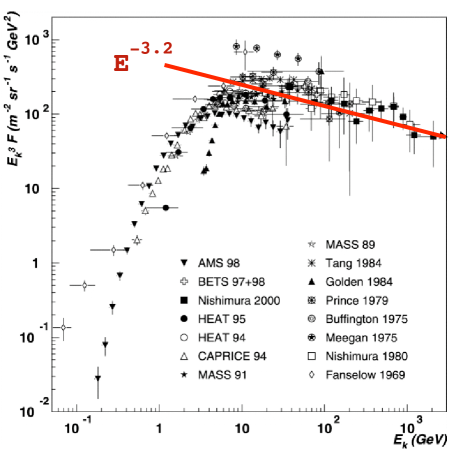
Figure 21: The CRE spectrum, summarized in Sapinski . The line is the central result of a power-fit to the higher-energy data; its slope is $3.2\pm 0.1$ Sreek .

Close inspection of Fig. 21 results in the conclusion that, for the most precise observations (the AMS experiment, AMS ), and at $E_{{}_{\rm eq}}\!\sim\!2.5$ GeV, the data are a factor $\sim\!2$ below the extrapolation to low energies of the predicted or best-fitted higher-energy behaviour of Eq. (68). The ‘diffusive’ energy-loss rate of Eq. (66) has the fastest growth with energy, after the radiative loss of Eq. (67). If we interpret $E_{{}_{\rm eq}}$ as the energy at which the corresponding characteristic times are equal, that is, if we equate $\tau_{\rm conf}^{e}$ in Eq. (65) to $\tau_{\gamma}$ in Eq. (69) at $E=E_{{}_{\rm eq}}$, we obtain:

$$K_{e}\sim 2\times 10^{8}\,\rm y,$$ (70)

as an estimate of the CR confinement time at $E\sim\!1$ GeV.

VIII The GBR

The existence of an isotropic, diffuse gamma background radiation (GBR) was first suggested by data from the SAS 2 satellite TF . The EGRET instrument on the Compton Gamma Ray Observatory confirmed this finding Sreek . We call “the GBR” the diffuse emission observed by EGRET by masking the galactic plane at latitudes $\rm{|b|\leq 10^{o}}$, as well as the galactic centre at $\rm{|b|\leq 30^{o}}$ for longitudes $\rm{|l|\leq 40^{o}}$, and by extrapolating to zero column density, to eliminate the $\pi^{0}$ and bremsstrahlung contributions to the observed radiation and to tame the model-dependence of the results. Outside this ‘mask’, the GBR flux integrated over all directions in the observed energy range of ${\rm 30}$ MeV to ${\rm 120~{}GeV}$, shown in Fig. 22, is well described by a power law $dF_{\gamma}/dE\!\propto\!E^{-2.10\pm 0.03}$ Sreek .

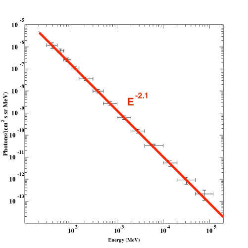
Figure 22: The GBR spectrum, measured by EGRET Sreek . The line is the central result of a power-law fit of slope $2.10\pm 0.03$.

The EGRET GBR data show a significant deviation from isotropy, correlated with the structure of the Galaxy and our position relative to its centre Anton ; DDDGBR2 . Contrariwise, the GBR’s spectral index is uncannily directionally uniform. These facts suggest a GBR which is partially local, as opposed to dominantly cosmological, and a common origin for the Galactic and extragalactic contributions.

In DDGBR we have analized the directional and spectral properties of the EGRET data and concluded that:

• The GBR is produced by ICS of CREs on starlight and the CBR.

• The GBR has comparable contributions from CREs in a Galactic halo of dimensions akin to the CR confinement volume discussed in Section V.12 (a directional and local source) and from other galaxies (an isotropic cosmological component).

• The contribution of active galactic nuclei (AGNs) to the GBR is at most comparable to that of the ensemble of external galaxies.

The first item implies that the GBR is a CR ‘secondary’: it behoves us to include it in a detailed discussion of CRs. To the third item, we dedicate Section VIII.3 below. The GBR’s spectral index, which we discuss next, is the same for the local and the cosmological contributions.

VIII.1 The GBR index

Consider the ICS of high energy electrons on starlight, of typical energy $\epsilon_{\star}\!\sim\!1$ eV, and on the CBR, whose mean current energyy is $\epsilon_{0}\!\approx\!2.7\,k\,T_{0}\!\approx\!0.64$ meV. The mean energy ${E_{\gamma}}$ of the Compton upscattered photons is:

$${E_{\gamma}(\epsilon_{i})\approx{4\over 3}\,\left({E_{e}\over m_{e}\,c^{2}}\right)^{2}\,\epsilon_{i}}\,,$$ (71)

with $\epsilon_{i}\!=\!\epsilon_{\star}$ or $\epsilon_{0}$.

The ICS photon spectrum originating in our galaxy is the sum of CBR and SL contributions. The ICS final-photon spectrum –a cumbersome convolution Felten of a CR power spectrum with a photon thermal distribution– can be approximated very simply. Using again the index “i” to label the CBR and SL fluxes:

$${dF^{i}_{\gamma}\over dE_{\gamma}}\propto{dE^{i}_{e}\over dE_{\gamma}}~{}\left[{dF_{e}\over dE_{e}}\right]_{E_{e}={E}_{e}^{i}}\;,$$

$${E}_{e}^{i}\equiv m_{e}c^{2}\sqrt{{3\,E_{\gamma}\over 4\,\epsilon_{i}}}\;,$$ (72)

where ${E_{e}^{i}}$ is obtained from Eqs. (71) by inverting ${E_{\gamma}(\epsilon_{i})}$. Introducing the CR-electron flux of Eq. (68) into Eqs. (72), we obtain:

$${dF^{i}_{\gamma}\over dE}\propto E^{-\beta_{\gamma}},$$

$$\beta_{\gamma}={\beta_{e}-1\over 2}\simeq 2.08.$$ (73)

The predicted index agrees with the measured one, ${2.10\pm 0.03}$ Sreek . Given Eq. (71), CREs of energy $E_{\rm CBR}\!\geq\!96$ GeV produce the GBR above 30 MeV by ICS of the current ($z\!=\!0$) CBR; CREs with energy $E_{\star}\!\geq\!2.4$ GeV suffice for ICS on starlight. For electrons of energy $E_{i}$, the radiation cooling times are $\tau_{\rm rad}(i)\!=\!3\,m_{e}^{2}\,c^{3}/(4\,\sigma_{{}_{\rm T}}\,E_{i}\,U_{i})$, so that locally $\tau_{\rm rad}(\star)\!\sim\!6\times 10^{8}$ y, and globally $\tau_{\rm rad}({\rm CBR})\!\sim\!1.3\times 10^{7}/(1+z)^{4}$ y. These numbers are much shorter than a Hubble time. ICS of CBR photons dominates the production of the extragalactic GBR, as we argue next.

VIII.2 The GBR flux and its directional-dependence

Adopt the standard cosmology and the usual notation ($H_{0},\,\Omega,\,\Omega_{M},\,\Omega_{\Lambda}$) for its parameters, specified in Appendix B.2. For a Galactic magnetic field $B\!\sim\!3\,\mu$G, $U_{{}_{B}}\!\sim\!U_{0}$; synchotron cooling and emission are locally relevant DDGBR ; DDDGBR2 . In our model, CBs transfer their kinetic energy to CRs all along their trajectories, which extend from the SN-rich inner galaxies to their halos and beyond. In galactic halos and galaxy clusters, $B\!<\!3\,\mu$G, and in the IGM, $B\sim 50\,$nG DDMF . In both places starlight is irrelevant, and ICS of the CBR, whose energy density increases with $z$ like $(1+z)^{4}$, dominates over synchrotron losses on the MFs. Thus, we calculate the intensity of the extragalactic GBR from the conclusion that the kinetic energy of CREs in the Universe with a lifetime shorter than the Hubble time has been converted by ICS of the CBR to $\gamma$-rays with the predicted spectrum of Eq. (73).

The main accelerators of high-energy CREs are SNe and the AGNs to be separately discussed in the next subsection. Other putative sources are negligible, as discussed in Appendix F for CRs in general.

The SN rate, $R_{{}_{\rm SN}}(z)$, is proportional to the star-formation rate, $R_{{}_{\rm SF}}(z)$, discussed in detail in Appendix B.4. Let $f_{{}_{\rm SN}}$ be the fraction of the luminosity in CREs out of the total luminosity $L_{{}_{\rm CR}}$ in CRs generated by SNe. The CB model does not currently imply a prediction for $f_{{}_{\rm SN}}$, which we assume to be equal to the ratio of the Milky Way’s luminosity in CREs to its total luminosity in CRs, i.e. $f_{{}_{\rm SN}}\!\sim\!1/40$.

Given our inferred 100% ICS conversion of CRE energy to photon energy, the GBR spectrum satisfies DDDGBR2 :

$$\!\!\int{dF_{\gamma}\over dE}\,E\,dE\!\approx\!{c\,f_{{}_{\rm SN}}\,L_{\rm CR}{\rm[MW]}\over 4\pi\,H_{0}\,R_{{}_{\rm SF}}(0)}\int\!{dz\,(1+z)^{-\beta_{s}}\,R_{{}_{\rm SF}}(z)\over\sqrt{\Omega_{M}\,(1+z)^{3}+\Omega_{\Lambda}}},$$ (74)

where $L_{\rm CR}{\rm[MW]}$ is specified in Eq. (21). Thus normalized, the spectrum of the contribution to the GBR from extragalactic SNe is estimated to be:

$${dF_{\gamma}\over dE}\simeq 0.9\times 10^{-3}\left[{E\over{\rm MeV}}\right]^{-2.08}{1\over\rm cm^{2}~{}s~{}sr~{}MeV}\;.$$ (75)

The GBR contains a considerable Galactic foreground due to ICS of CBR, starlight and sunlight photons by Galactic CREs. The convolution of a CRE power-law spectrum with a photon thermal distribution Felten can be approximated very simply DDGBR ; DDDGBR2 . Using the index $i$ to label the CBR, starlight and sunlight fluxes, we have:

$${dF_{\gamma}\over dE_{\gamma}}\simeq N_{i}(b,l)~{}\sigma_{{}_{\rm T}}\,{dF_{\gamma}^{i}\over dE_{\gamma}},$$ (76)

where $N_{i}(b,l)$ is the column density of the radiation field weighted by the distribution of CREs in the direction $(b,\,l)$, and the $dF_{\gamma}^{i}/dE_{\gamma}$ are as in Eq. (72). The distribution of the non-solar starlight is approximated as $\propto 1/r^{2}$, with $r$ the distance to the Galactic centre, and the CREs are assumed to be distributed as a Gaussian “CR halo” DDGBR . Naturally, the results depend crucially on the size and shape of this halo. We use a Gaussian distribution with a scale length of $\rho_{e}\!=\!35$ kpc in the Galactic disk and a scale height of $h_{e}\!=\!8$ kpc perpendicular to the disk DDDGBR2 . The justification for this choice of $h_{e}$ is the following. The radio emission of “edge-on” galaxies –interpreted as synchrotron radiation by electrons on their magnetic fields– offers direct observational evidence for CREs well above galactic disks, see, e.g. Ref. Duric1998 . For the particularly well observed case of NGC 5755, the exponential scale height of the synchrotron radiation is ${\cal{O}}(4)$ kpc. If their energies are in equipartition, CRs and MFs should have similar distributions, and the Gaussian scale height, ${h_{e}}$, of the electrons ought to be roughly twice that of the synchrotron intensity, which reflects the convolution of the electron- and magnetic-field distributions. The inferred value is ${h_{e}}\sim 8$ kpc.

Due to Feynman scaling, the GBR from $\pi^{0}$ production and decay in hadronic CR collisions in the ISM and IGM has the same power-law index as that of CRs Dar1995 , i.e. $-2.77$ in the ISM of galaxies and $-2.17$ in the IGM inside and outside galaxy clusters. This contribution to the extragalactic GBR is much smaller than that of CREs.

In Fig. 23 we compare the observed GBR with our predictions, as functions of Galactic coordinates. The prediction is a sum of a $(b,\,l)$-dependent Galactic foreground produced by ICS of the CBR, starlight and sunlight, and a uniform extragalactic GBR. The result has $\chi^{2}/{\rm dof}\!=\!0.85$, a vast improvement over the constant GBR fit by EGRET, for which $\chi^{2}/{\rm dof}\!=\!2.6$. The ratios of $l$-integrated extragalactic to galactic fluxes are $\sim\!0.5$, 0.9, 1.5, for $|b|=20^{\rm o}$, $45^{\rm o}$, $75^{\rm o}$. The ‘foreground’ component of the $\gamma$ ‘background’ is $\sim\!50\%$ of the total radiation.

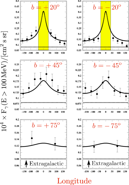
Figure 23: The flux of GBR photons above 100 MeV: comparison between EGRET data and our model for ${h_{e}\!=\!8}$ kpc, ${\rm\rho_{e}\!=35\!}$ kpc, as functions of longitude $l$ at fixed latitudes $b$. The shaded domain is EGRET’s mask. Notice that the vertical scales do not start at zero.

We conclude that the GBR can be explained by standard physics, namely, ICS of CBR and starlight by CREs from core-collapse SNe. At $E_{\gamma}\!>\!100$ GeV, most of the extragalactic GBR is absorbed by pair production on the Cosmic Microwave Background (CMB) Salamon and the diffuse GBR reduces to the Galactic foreground. This suppression, and a decisive determination of the angular dependence in Fig. 2, should be observable by GLAST.

VIII.3 The contribution of AGNs to the GBR

Active galactic nuclei, powered by mass accretion onto massive black holes, eject powerful relativistic jets, mainly during their $\sim 10^{8}$ y bright phase around $z\!=\!2.5$. The CBs of these jets should generate CR electrons and nuclei in precisely the same way as the CBs from SNe do. The kinetic power of AGN jets has been estimated from their radio lobes, assuming equipartition between CR energy and MF energy, and a ratio of CR electrons to CR nuclei similar to that observed in our Galaxy. Kronberg et al. Kronberg , for instance, have estimated that ‘giant’ extragalactic radio sources, powered by accretion onto massive black holes ($M>10^{8}\,M_{\odot}$), inject $10^{61}$ to $10^{62}$ erg into radio lobes. Such powerful CR sources may contribute to the observed spectrum of CRs. The most reliable estimate of the contribution to the CR flux, discussed in the next Section, may be the estimate that parallels the study of the relative contribution of external galaxies and AGNs to the GBR, which we discuss next DDDGBR2 .

In search of an upper bound, we assume that the kinetic energy release in relativistic jets is the maximal energy release from mass accretion onto a Kerr black hole ($\approx\!42\%$ of its mass), and that this energy is equipartitioned between magnetic fields and cosmic rays with a fraction $f_{{}_{\rm AGN}}$ of the CR energy carried by electrons. These CREs also cool rapidly by ICS of the CBR. The energy of CREs whose radiative cooling rate, $\tau_{\rm rad}(z)$, is larger than the cosmic expansion rate, $H(z)$, is converted to $\gamma$-rays. Their energy is redshifted by $1+z$ by the cosmic expansion. Using a black hole density, $\rho_{{}_{\rm BH}}(z=0)\!\sim\!2\times 10^{5}\,M_{\odot}\,{\rm Mpc^{-3}}$ in the current Universe Tremaine , and the CB-model injection spectral index, $\beta_{s}=13/6$ of Eq. (52), we estimate a contribution from AGNs to the extragalactic GBR flux:

$${dF_{\gamma}\over dE}<{2.4\times 10^{-3}\,c\,f_{{}_{\rm AGN}}\,\rho_{{}_{\rm BH}}\,c^{2}\over 4\,\pi\,{\rm MeV}}\left[{E\over{\rm MeV}}\right]^{-2.08}\,,$$ (77)

where, again looking for a bound, we have neglected the cosmological redshift of the GBR energy. With the above priors, Eq. (77) corresponds to a spectrum:

$${dF_{\gamma}\over dE}\simeq 4.0\times 10^{-4}\left[{E\over{\rm MeV}}\right]^{-2.08}~{}{f_{{}_{\rm AGN}}/f_{{}_{\rm SN}}\over\rm cm^{2}~{}s~{}sr~{}MeV}\,.$$ (78)

For an assumed $f_{{}_{\rm AGN}}\!\sim\!f_{{}_{\rm SN}}$, Eq. (78) bounds the contribution of AGNs to $<\!44$% of that of extragalactic SNe, Eq. (75). It is clear from the derivation of this result that it is at best ‘an estimate of an upper bound’. On the other hand, the successful study of the GBR in DDDGBR2 —wherein the AGN contribution is neglected— implies that the bound cannot be significantly violated.

In DDDGBR2 we discussed the contribution of various established point sources to the GBR, concluding that they cannot explain its origin. The fact that all the AGNs detected by EGRET are blazars led various authors to suggest that these objects are the main sources of the GBR Bignami ; Chiang . Subsequent studies have shown that at most 25% of the GBR can result from unresolved blazars Mukherjee , i.e. AGNs pointing close to our direction. The contribution from the much more abundant AGNs not pointing to us, is much more important DDDGBR2 .

IX The contribution of AGNs to UHECRs

A comparison between the contributions of AGNs and extragalactic SNe to the UHECR flux can be made along the same lines as in Section VIII.3. Assuming that the source spectra of these contributions have the same energy dependence, the end result is the same: the AGN flux cannot be much bigger than $\sim\!44$% of the extragalactic core-collapse SN flux. This is because the tribulations (discussed in Section VIII.3) that CRs of either source suffer on their way are the same. In particular, because of the effect of the GZK cutoff, UHECRs reach us from a look-back time (or redshift) much smaller than that of the extragalactic contribution to the GBR, but that ‘finite-volume’ effect drops from the ratio of the fluxes, in the approximation in which the matter of the universe is uniformly distributed.

X Recent Data

We call ‘recent’ the observations that have been published after the first posting of the current paper in June 2006. On the realm of GRBs, on which our theory of CRs rests, enormous progress has been made in the observations, particularly in the X-ray domain, with the help of the Swift satellite Swift , amongst others. Concerning the CR domain, the novelties include data from HIRES HIRESGZK on the GZK cutoff, from the Tibet AS$\gamma$ collaboration on CRs in the knee region Amenomori ; TibetpHe , from the Pierre Auger collaboration on UHECRs Mello ; Unger ; PAC , and from the HESS and MAGIC collaborations on $\gamma$-ray astronomy Ribo . We comment on these data in view of our original results.

X.1 GRBs in the “Swift era”

Various satellites are currently contributing to a wealth of new data on GRBs and XRFs. Swift, a true technological jewel, is one of them. With nominal celerity, Swift has filled a gap in GRB data: the very ‘prompt’ X-ray and optical radiations, and very precise measurements of X-ray afterglows at later times. The recent data fully corroborate the CB model of GRBs and XRFs.

A very simple result concerns the predicted correlations between “prompt” GRB observables DDOldCorr . These follow directly from the kinematics underlying the assumption that a GRB’s $\gamma$-rays are produced by ICS of ‘ambient-light’ photons, see Section II.1 and Appendix D. Consider the “peak energy”, $E_{p}$, of GRBs and XRFs and their “isotropic-equivalent” energy, $E_{\rm iso}$. For a point-like source $(1+z)\,E_{p}\!\propto\!\gamma\,\delta$ and $E_{\rm iso}\!\propto\!\delta^{3}$, with $\delta$ the Doppler factor of Eq. 121, which varies extremely rapidly as a function of the observer’s viewing angle $\theta$. If that large and inevitable case-by-case variation is the dominant one, we expect $(1+z)\,E_{p}\!\propto\!E_{\rm iso}^{1/3}$. A CB initially expands in its rest system at a speed of ${\cal{O}}(c)$, so that in its motion it traces a cone of aperture of ${\cal{O}}(1/\gamma)$. By ICS, its interacting electrons emit radiation also within a forward angle of ${\cal{O}}(1/\gamma)$. For energetic GRBs, viewed at angles of ${\cal{O}}(1/\gamma)$, the volume-averaged Doppler factor is $\delta\!\propto\!\gamma$, so that the case-by-case variation of $\gamma$ results in the expectation $(1+z)\,E_{p}\!\propto\!E_{\rm iso}^{2/3}$. The transition from a 1/3 to a 2/3 slope is precisely what is seen in Fig. 24a. The crossed lines are the expectation for a “typical” GRB DD . The predicted correlations are also verified by the data for a handful of other pairs of observables DDDCorrelations .

Swift has established the predicted AGoptical ; AGradio canonical behaviour of the X-ray and optical AGs of a large fraction of GRBs. The X-ray fluence decreases very fast after the ‘prompt’ peaks of the GRB. It subsequently turns into a ‘plateau’. After a time of ${\cal{O}}(1$d), the fluence bends (has a ‘break’, in the usual parlance) steepening to a power-decline. In Fig. 24b, this is shown for a Swift GRB DDDBreaks , and compared with the CB-model expectation. The early peaks are produced by ICS by a succession of CBs, that become ‘weaker’ as the accreting material that generates them is exhausted. The plateau is due to the dominant CB, as it coasts in the ISM and synchrotron-radiates the energy of the ISM electrons that it intercepts. The end decline reflects the deceleration of the CB in the ISM.

The rapid transition from ICS to synchrotron-radiation dominance in the X-ray light curves is accompanied by an abrupt change of spectral behaviour AGoptical ; DD . This is illustrated in Fig. 24c where the radiation’s spectral index, $\Gamma$, is shown and compared with the model’s expectation DDDDecline . The time dependence of the AG’s flux and its spectral index are related for individual GRBs as in Eq. (134). The test of the predicted relation is shown in Fig. 25a.

Figure 24: Top (a). The correlation between $(1+z)\,E_{p}$ and $E_{\rm iso}$. The “official” distinction in terms of $E_{p}$ between GRBs and XRFs is shown. The red cross marks the average expectations for GRBs. The red star is XRF 060218. Middle (b). The X-ray light curve of GRB 060729. The transition from Compton to synchrotron dominance is at the start of the flat “plateau”. Botton (c). Time evolution of the X-ray spectral index $\Gamma$ ($dN_{\gamma}/dE\!\approx\!E^{-\Gamma}$) of the same GRB, with the transition occurring at the same time.

As explained in Appendix D.5, the ambient light around a just-exploded SN has a “thin bremsstrahlung” spectrum $dN_{\gamma}/dE_{i}\!\propto\!(1/E_{i})\,{\rm Exp}[-E_{i}/T_{i}]$, with $T_{i}$ a pseudo-temperature. The electrons in a CB boost this light by ICS to a GRB spectrum with the same shape and a higher final $T_{f}\!\propto\!\gamma\,\delta\,T_{i}$. On occasion a GRB or an XRF is dominated by a single CB, and its analysis is particularly simple. One example is XRF 060218, the star in Fig. 24a. For this XRF one may use the observed X-ray ‘peak energy flux’ of its single-peak X-ray light curve to predict the corresponding fluxes of its (much broader) UV and optical peaks, also produced via ICS of ambient light by the CB DDDXrays ; DNature . This is done in Fig. 25b. The ambient light sampled by a CB becomes increasingly radially-directed with distance from the SN, $r$, so that the incident angle of photons, $\theta_{i}$, on the CB’s electrons obeys $\langle 1+\cos\theta_{i}\rangle\!\to\!1/r^{2}$; and $T_{f}\!\propto\!\langle 1+\cos\theta_{i}\rangle\!\to\!1/r^{2}$. In the “prompt” phase, while a CB has not significantly decelerated, $r\!\propto\!t$, the observer’s time. To a fair approximation, then, the time-energy correlation of the spectrum is such that $E\,dN/(dE\,dt)\!\propto\!F(E\,t^{2})$. This ‘$E\,t^{2}$ law’ is tested in Fig. 25c for the “peak times” of the XRF’s pulse at frequencies ranging from X-rays to optical DDDXrays .

Figure 25: Top (a). Test of the relation between the “index” $\beta_{\rm ac}$ governing the whole spectral evolution of the X-ray synchrotron AG, and the index of its spectrum, Eq. (134). Middle (b). Test of the “peak-energy fluxes” in UV and optical intervals predicted from the same observable in the X-ray domain, for the single-peak XRF 060218. Data and predictions have been slightly shifted for clarity. Bottom (c). Test of the correlation between peak times and energy for the same XRF, in a wide domain. The line is the approximate “$E\,t^{2}$ law”, $t_{0}$ is the energy-independent pulse start-time.

The Swift data display a panoply of X-ray AG shapes, ranging from some having a long and very flat plateau to others well approximated at all times by a single power law. In the CB model this is the prediction of Eq. 133. A GRB pointing close to the observer ($\theta\,\gamma_{0}\!<\!1$) is very luminous, its radiation being highly Doppler boosted, see Eq. 120. Its synchrotron radiation diminishes uniformly as $\gamma(t)$ and $\delta(t)$ decrease, resulting in an approximately power-law AG. A GRB pointing away from the observer’s direction ($\theta\,\gamma_{0}\gg 1$) is relatively under-luminous (and is often classified as an XRF) because its beam is forward-collimated within an angle $1/\gamma$. As $\gamma$ diminishes the beam opens up to reach the observer, resulting in a plateau or even an increased radiation. Finally $\gamma(t)$ and $\delta(t)$ become small enough for the AG to tend to a power law. Studied in detail, these simple facts reproduce the entire panoply of observed light-curve shapes DDDBreaks .

The successful analysis of “Swift-era” data that we have briefly illustrated is entirely based on predictions made before the launch of Swift. From the CB-model’s point of view the data of this era has taught us two things. First, during the fast decline of the X-ray flux, and sometimes later, one can occasionally see the effects of late and “weak” CBs, the dying pangs of their accretion-governed “engine”. Second, the bremsstrahlung and line-emission phase cited in Appendix D.6 may be generally subdominant: a simplification.

X.2 Tibet AS$\gamma$

This group has studied the all-particle spectrum in the energy range of $\sim\!10^{5}$ to $\sim\!10^{8}$ GeV, finding it to be compatible with measurements from previous experiments Amenomori . It has also analyzed in detail the p and He spectra around their knees TibetpHe . Their results are shown in Fig. 26, superimposed on the (red) curves of Fig. 15.

Figure 26: The proton (Top) and He (Bottom) spectra around their ‘knees’, obtained by the Tibet AS$\gamma$ collaboration Amenomori . The (red) curves are those of Fig. 15.

X.3 HIRES and Auger

The HIRES collaboration has announced the observation of the GZK cutoff HIRESGZK . The Pierre Auger observatory in Argentina has improved the precision of the data on UHECRs Mello , studied their composition Unger , and reportedly located some of their sources PAC .

The UHECR all-particle spectrum of Auger is shown in Fig. 27. The upper curve in this figure is the same as the (blue) curve in Fig. 13; if shifted down in flux by a factor $\sim\!1.7$, it results in the lower curve. This is the overall factor by which the Northern-hemisphere data of Fig. 13 exceed the Southern-hemisphere ones. This difference may be due to the well-known calibration difficulties. It may also be real, for the Northern sky is, within a radius of the order of the distance to the Virgo Cluster, more densely populated that the Southern sky. If CRs above the Ankle are mainly extragalactic, and if the MFs they cross are insufficient to scramble completely their arrival directions, one would expect a higher Northern flux.

Figure 27: The Auger UHECR spectrum Mello . The upper curve is the same as the (blue) curve in Fig. 13. The lower curve is the same one, but shifted down in flux by a factor $\sim\!1.7$.

The Auger data on $X_{\rm max}(E)$ Unger are compared with previous observations in Fig. 28. The blue line is that of Fig. 18, in which one can ascertain the dependence of the expectations on various Monte-Carlo (MC) simulations. The dashed line, which agrees with the Fly’s eye results, is the same blue curve, rescaled down in $X_{\rm max}$ by 2.3%, well within the MC uncertainties. The green line, which agrees with the Auger data, is the blue line, shifted in $dX_{\rm max}/d\,{\rm Log}_{10}(E)$ by 3.3% per decade of energy, not larger than the difference in slope from some MCs to others. These considerations illustrate how difficult it is to extract the CR composition at large $E$. Note that changes in composition are easier to ascertain, since changes in the slope of $X_{\rm max}(E)$ clearly reflect them. The Auger results have a clear change of slope at the Ankle, as expected in our model. Note also that the MC-to-MC spread in $dX_{\rm max}/d\,{\rm Log}_{10}(E)$ is much smaller than that of $X_{\rm max}$ itself. It might be useful to study $dX_{\rm max}/d\,{\rm Log}_{10}(E)$, which would signal compositional changes in a much-reduced MC-dependent way.

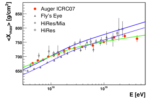
Figure 28: The trend of $X_{\rm max}(E)$ at very high energies. Data from Auger are compared with those of previous experiments Unger . The blue line is that in Fig. 18, the others are commented in the text.

X.4 Auger’s directional correlation with AGNs

The Auger collaboration has reported PAC a correlation between arrival directions of UHECRs and nearby AGNs from the Véron catalog Veron . The effect is maximized for events with $E\!>\!57$ EeV $\!=\!5.7\times 10^{10}$ GeV, and a $3.1^{\rm o}$ aperture around AGNs with $z\!<\!0.018$, corresponding to a distance $D\!<\!75$ Mpc along a straight trajectory, smaller than the corresponding distance, $D\!=\!200$ Mpc, to the GZK “horizon”, defined in Ref. PAC by a 10% attenuation of protons with $E_{p}\!>\!60$ EeV. In the optimized sample some 20 events are correlated and $\sim\!1/3$ as many are not. The collaboration cautiously warns that AGNs could be mere tracers of the density distribution of matter.

As we saw in Section IX, if AGNs accelerate CRs the way that core-collapse SNe allegedly do, an AGN contribution to UHECRs could be significant. That is a correct statement for the angularly-integrated flux, but not for the flux from 20 arrival directions of $3.1^{\rm o}$ aperture, which ought to be, on pure geometrical grounds, significantly smaller. Neither do we expect the matter-density enhancement traced by AGNs to correspond to a sufficient number of SNe, close to AGNs, and emitting jets pointing close to our direction.

Other difficulties in our understanding of the Auger data are more model-independent. The Véron catalog is not directionally uniform in its coverage and sensitivity, unlike the Auger coverage within its field of view. A $3.1^{\rm o}$ deviation is of the order of magnitude of that inflicted on UHECRs by the MF of the Galaxy, it would be surprising if extragalactic CRs did not encounter other MFs with similar or larger effects. The Auger correlation is purely directional, not investigated case-by-case for the possible effects of AGN distance, luminosity, jet direction and radio loudness. The effect of distance is obvious, the correlation with luminosity is very plausible. Concerning jet-direction, one has to understand how the UHECRs from AGNs could be fairly isotropically emitted, given that AGNs produce extremely collimated jets, and that they are seen in $\gamma$-rays as very luminous blazars when the jets are pointing in our direction. The proton- and electron-acceleration efficiencies of CR sources are presumably correlated. The radio loudness is a measure of the electron-acceleration efficiency, since the radio signal, as in Fig. 2b, is due to synchrotron-radiating electrons. Finally, the number of UHECR Auger events is roughly the same in each of five equal-exposure domains, but the AGNs of the Véron catalog, which cluster along the super-galactic plane, are differently distributed.

For the above reasons we do not attempt to adapt at the moment our model to the Auger findings, limiting ourselves to the few comments that follow.

The CBs of AGNs are much more massive than those of SNe, but their Lorentz factors, estimated from their superluminal motion gammaAGN , are much smaller, $\gamma\!=\!{\cal{O}}(10)$. Their observed SR was used to estimate a field $B\!=\!{\cal{O}}(1\,\rm mG)$ MFAGN . This is precisely consistent with the equipartition estimate, $B\!\sim\!\gamma\,\sqrt{8\,\pi\,n\,m_{p}\,c^{2}}$, for $\gamma\!=\!10$ and the mean IGM baryon density, $n\!\sim\!2.3\times 10^{-7}\,{\rm cm^{-3}}$ determined from the observations of WMAP WMAPdens .

The CBs of an AGN may ‘inelastically’ accelerate CRs to well above the GZK limit and collimate them forward in a cone of aperture $\theta\!\sim\!1/\gamma$. In view of the Auger results, we are interested in a potentially more isotropic source, the end ‘lobe’ of an AGN jet being the obvious choice LobeCRs . These lobes have radii $R_{L}$ of a few kpc. They are steadily energized by the incoming CBs. Traveling in a medium swept up by previous CBs, a jet may deposit in its lobe half of the energy, $E_{\rm AGN}\!=\!{\cal{O}}(10^{60}\,\rm erg)$, emitted by the central black hole during the AGN’s active life. In equipartition, $E_{\rm AGN}\!=\!(2/3)\,B_{L}^{2}\,R_{L}^{3}$, corresponding to a field $B_{L}\!=\!{\cal{O}}(1\,\rm mG)$. The larmor-limit energy for the acceleration of a proton in a lobe is then $E_{\rm max}\sim e\,B_{L}\,R_{L}\!\approx\!3\!\times\!10^{21}\,{\rm eV}$, above the GZK cutoff.

The analogy with AGN jets is one of the items originally inspiring the CB model. Perhaps the Auger results may be used to close this analogy into a loop. If AGNs are tracers of very dense environments, it is conceivable that the jets of nearby SNe stop swiftly in mini-lobes, much as the non-relastivistic ejecta of SNe are sometimes observed to clash with molecular clouds W41 ; 443 . The CRs from these mini-lobes would not be forward-collimated. This would make core-collapse SNe in AGN environments potential sources of the UHECRs observed by Auger.

X.5 TeV $\gamma$-rays from supernova remnants

Various observatories, HESS, MAGIC, CANGAROO-III and VERITAS Ribo are currently charting the sky for ‘TeV’ $\gamma$-ray sources, following a multi-telescope Cherenkov technique pioneered by HEGRA Pulhofer . Their data may test, among other things, the earlier claims from X-ray observations Koyama that SNRs are ‘Tevatrons’.

The HESS system in Namibia has surveyed the Galactic plane at latitudes $\rm{|b|\leq 6^{o}}$ and longitudes $\rm{-85\leq|l|\leq 60^{o}}$, for $\gamma$-rays between 100 GeV and several tens of TeV. It has found dozens of sources, many of them previously unknown, and having no known counterpart at other wavelengths Hoppe . HESS also detected TeV $\gamma$ rays from three SNRs. The collaboration concludes that “The paradigm of CR acceleration in Supernova remnants (SNRs) is consistent with our new findings” but is cautious in adding “but it seems clear that the new sources are not drawn from a single population” Aharonian . If the cited “paradigm” includes the consuetudinary contention that the bulk of non-solar CRs below the knee(s) is accelerated by SNRs (see, e.g. Ref. Drury ), we, and others Plaga , beg to disagree.

In the conventional view, a non-relativistic spherical shell ejected in a SN explosion drives a strong shock into the ambient medium, heating it up to a multi-keV temperature, and accelerating ions and electrons to CR energies. The ionized gas emits thermal X-rays via bremsstrahlung. The accelerated CR electrons emit non-thermal SR extending from the radio to the X-ray band. They also emit $\gamma$ rays by ICS of the locally-generated radiations. The accelerated CR nuclei emit $\gamma$ rays and neutrinos from the decay of mesons produced by hadronic collisions in the ejecta and in the ambient plasma.

Although SNRs are well established as non-thermal sources of radio, X- and $\gamma$-rays, as well as thermal sources of soft X-rays, the observations do not support the basic relations for the CR-accelerating shocks driven by the SN shells into the ionized ISM. The shock velocity, $V_{s}$, and the ISM temperature behind the shock, $T_{s}$, for instance, ought to be related by $k\,T_{s}=(3/16)\,\mu\,m_{p}\,V_{s}^{2}$, with $\mu\!\sim\!0.6$ the mean plasma mass in $m_{p}$ units. This expectation is badly disobeyed by young SNRs, a result interpreted as evidence for an efficient (though unobserved) acceleration by shocks of modified structure and hydrodynamics Ellison .

Radio SR has been observed from many Type II and Type Ib/c SNe, but no SN Ia has yet been detected as a radio emitter, even when observed quite promptly or quite nearby Panagia . This implies that efficient CR acceleration and the generation of the required strong MFs must involve collisions of SN shells with targets much denser than the average ISM. Such high-density targets, unlike the low-density ISM around SNe Ia, can be provided by massive ejecta or winds from the progenitor star of core-collapse SNe, or by the high-density molecular-cloud environment in which some Type II SNe take place. Collisions with such over-dense targets can produce intense turbulent MFs in the expanding SN shell. If the MF is in energy equipartition with ejecta of velocity $V_{\rm ej}\!\equiv\!\beta_{\rm ej}\,10^{-2}\,c$, impinging on a medium of density $n\!\equiv\!n_{1}\,{\rm cm}^{-3}$, the MF intensity is $B_{\rm eq}\!\sim\!0.7\,\beta_{\rm ej}\,\sqrt{n_{1}}$ mG. In principle, such strong magnetic fields can very efficiently accelerate ions and electrons to CR energies via the Fermi mechanism. The accelerated CR nuclei and electrons can produce TeV $\gamma$ rays by hadronic interactions and by ICS of ambient photons, respectively.

Two SNRs displaying a shell morphology at TeV energies have been found by HESS: RX J1713.7-3946 3946 and RX J0852-4622 4622 . The TeV shells seem to follow the SR keV emission pattern seen by X-ray satellites, suggesting ICS of ambient photons as the origin of the TeV emission. On the other hand, TeV emission has also been found in two SNRs, HESS J1834087/W41 W41 and MAGIC J0616+225/IC 443 443 , in the interaction region between the SNRs and molecular clouds, suggesting a hadronic origin. Combining this information with the absence of radio emission from SNe Ia, leads us to conclude that the molecular clouds do not only serve as gas targets converting hadronic CRs from adjacent SNRs to TeV $\gamma$ rays, but that the acceleration itself takes place in the collision region between the SN shell and the molecular cloud. Such $\gamma$-ray Tevatrons are very rare among the $\sim\!250$ SNRs observed in the Galaxy. This implies that the total production rate of CR nuclei in SNRs falls very short of supplying the observed Galactic CR luminosity. This conclusion is consistent with two other facts: The distribution of Galactic CRs –as inferred from the distribution of diffuse $\gamma$ radiation from the Galactic disk– has a scale hight and radius much larger than expected from the interactions of CRs from SNRs in the Galactic ISM. Non-solar CRs do not show the anisotropy of arrival directions near Earth expected from the location of the solar system, relative to the distribution of SNRs Smith .

X.6 TeV $\gamma$-rays from GRBs

The typical or “peak” energies of the prompt $\gamma$- rays of GRBs are of the order of a few hundred keV. This agrees with the prediction of the CB model DD , $(1+z)\,E_{p}\!\sim\!\gamma_{0}\,\delta_{0}\,T_{i}/2$, with $T_{i}\!\sim\!1$ eV the pseudo-temperature of the glory’s thin bremsstrahlung spectrum. In this model there are two sources of higher-energy photons, one during the prompt phase, the other during the AG phase.

The CR electrons accelerated by a CB during the prompt phase have an average Lorentz factor $\Gamma_{e}\!\sim\!\gamma_{0}^{2}$. They Compton up-scatter the glory’s photons to a distribution with the same spectral shape as the bulk of the GRB’s prompt $\gamma$’s, but with a characteristic ‘second’ peak energy $(1+z)\,E^{\prime}_{p}\!\sim\!\gamma_{0}^{2}\,\delta_{0}^{2}\,T_{i}/2$. This is typically a million times larger than $(1+z)\,E_{p}$, that is, in the range of hundreds of GeV DDS05 . The relative flux of this hard prompt component is difficult to estimate. It may have been seen in the case of GRB 980425 DDS05 , observed very nearby but at a relatively very large observer’s angle (small $\delta_{0}$). The satellite GLAST may be able to detect these prompt high-energy photons.

In the AG phase, CR nuclei accelerated by the CB, mainly protons, impinge on ISM nuclei to produce $\pi^{0}$’s, and thus $\gamma$’s in their $\pi^{0}\to\gamma\gamma$ decay. The calculation of an upper limit to the $\gamma$ flux is straightforward. An estimate of the actual flux is practically impossible, mainly because we cannot confidently ascertain the broadening of the proton ‘beam’ by magnetic fields, before the beam encounters its target ‘beam dump’. We discuss in turn the flux upper limit, its potential decrease by beam broadening, and an optimistic scenario in which the CBs themselves are the beam dump.

At incident TeV energies, the total inelastic proton-nucleon cross section is $\sigma_{\rm in}\!\simeq\!40$ mbarn. The column density of an effective beam dump –in which the fraction of protons that collide is large– is a reference $N_{\rm eff}\!\sim\!1/\sigma_{\rm in}\!\simeq\!2.5\times 10^{25}$ nucleons/cm², much larger than the values we shall deal with (the astrophysical dumps relevant to our discussion are thin enough for TeV photons not to be significantly absorbed, though, traveling for longer cosmological distances, they may be attenuated by pair production in the cosmic infrared background).

The column densities extracted from the fitted X-ray absorption as a function of energy, for GRBs observed by Swift SwiftAtt , vary within an order of magnitude of $N_{\rm Swift}\!\sim\!10^{21}$ nucleons/cm². The CR protons made by a CB also traverse this dump, which is “thin”. Indeed, the probability of a TeV proton to interact while in the host galaxy, assuming that all the extragalactic X-ray absorption took place in it, is $N_{\rm Swift}/N_{\rm eff}\!\ll\!1$. The proton beam carries the energy of a single average jet of CBs, 1/2 of the result of Eq. (18). Its spectral index is that of the “source” flux, Eq. (52), since the effects of accumulation in the magnetic field of the parent galaxy have not yet affected it. Therefore, the proton number flux is:

$${dn_{p}\over dE}\approx 1.25\times 10^{53}\;{\rm GeV}^{-1}\left({{\rm GeV}\over E}\right)^{\beta_{s}}$$ (79)

To a very good approximation, the $\gamma$ flux generated by a power-law proton beam, such as that of Eq. (79), impinging on a thin dump, has the same energy dependence as the proton beam, and a fraction $F_{p\to\gamma}\!\sim\!0.04$ of its normalization (per interacting proton) at a given energy nubeam . For a GRB whose beam dump’s column density is $N_{{}_{\rm GRB}}$, the $\gamma$ number-flux is:

$${dn_{\gamma}\over dE} \approx N_{{}_{\rm GRB}}\,\sigma_{\rm in}\;F_{p\to\gamma}\;{dn_{p}\over dE}$$ (80)

$$\sim {2.0\times 10^{48}\over{\rm GeV}}\,{N_{{}_{\rm GRB}}\over N_{\rm Swift}}\left({{\rm GeV}\over E}\right)^{\beta_{s}}$$

At a given point in time the number-flux of photons is enhanced in the forward direction be the factor $\delta^{2}(\gamma,\,\theta)$ of Eqs. (120, 121). In search for an upper limit, we shall illustrate the forward case, $\theta\!=\!0$, for which $\delta(t)\!=\!2\,\gamma(t)$, a good approximation in all cases as soon as $\gamma(t)$ becomes small enough to satisfy $\theta\,\gamma(t)\!<\!1$. In the same search for an upper limit, we integrate over all of the trajectory of a CB, or all the CRs that it accelerates, till $\gamma(t)\!\sim\!{\cal{O}}(1)$, with the help of Eq. (8). At $\theta\!=\!0$, this means that the instantaneous $\delta^{2}$ is to be traded for an integral:

$$\langle\delta^{2}\rangle\simeq\gamma_{0}\,\int_{\gamma_{0}}^{\sim 1}{(2\,\gamma)^{2}\over\gamma^{3}}\,d\gamma\simeq 4\,\gamma_{0}\,\ln{\gamma_{0}}$$ (81)

For a GRB at a luminosity distance $D_{L}(z)$, the $\gamma$ flux per unit area and energy is:

$$\!\!\!\!\!\!\!\!{dF_{\gamma}\over dE}\approx{(1+z)\,\langle\delta^{2}\rangle\over 4\,\pi\,D_{L}^{2}}\;{dn_{\gamma}\over dE}\biggl{|}_{E\rightarrow(1+z)E}$$

$$\!\!\!\!\!\!\!\!\sim{4.6\times 10^{-4}\over{(1+z)^{0.2}\,\rm GeV\,cm^{2}}}\;{N_{{}_{\rm GRB}}\over N_{\rm Swift}}\left({{\rm GeV}\over E}\right)^{2.2}\left({{\rm Gpc}\over D_{L}}\right)^{2}$$ (82)

where we have approximated $\beta_{s}\!\sim\!2.2$ and specified the result for $\gamma_{0}\!=\!10^{3}$. This flux is integrated in time for the duration of the GRB’s AG, typically of order months.

The flux of Eq. (82) is not large. For example, for $z\!=\!1$ [$D_{L}(z)\!\approx\!7.1$ Gpc, for standard cosmological parameters], and above a threshold of 250 GeV, it corresponds to $\sim\!8.8\times 10^{-9}$ photons per cm², below the sensitivity threshold of current Cherenkov telescopes, for a signal spread over more than a few days. Moreover, there are four other reasons why Eq. (82) is but an upper limit:

First, we have worked in the limits wherein all CRs are generated before they hit the dump.

Second, we have assumed that the primary proton flux is isotropic in the CB’s rest system. For non-singular angular distributions, this does not affect the derived spectral shape of Eqs. (52, 53). But reasonable distributions favouring forward proton-CB scattering in the CB’s system would result in a less forward-peaked proton beam in the SN rest system, and in a beam of $\gamma$’s less forward-collimated than reflected by the factor $\langle\delta^{2}\rangle$ in Eq. (82). This may reduce the flux by a factor of a few.

Third, the inter-stellar MFs encountered by TeV protons could widen the proton beam by many degrees, before it interacts with the ISM to produce $\gamma$ rays. This would decrease the flux of Eq. (82) by orders of magnitude. Yet, the energy density of the CR beam preceding a CB in its trajectory is so very many orders of magnitude larger than the energy density of the typical ISM field, that the beam ought to wipe out the MF within a funnel of angular aperture $\sim\!1/\gamma$ DDMFWipeout . The CB-generated CRs exiting a CB at a given point in its trajectory would travel straight in the MF-free domain produced by CRs having exited the CB before. That is only correct on average, for the CRs emitted at a larger than average angle would escape into a domain with conventional MFs. So would the CRs at the leading front of the funnel, even if, before they escape, they are repeatedly caught up and reaccelerated by the CB Hillas . This process is too complex to be understood in detail. But we know observationally that CR electrons escape into the space surrounding a beam of CBs, see, e.g. Fig. (2b).

Fourth, photon attenuation of TeV photons by pair production on the infrared background radiation is very strong at redshifts in excess of $z\!\sim\!0.1$ Stecker .

A uniform-density CB with the initial baryon number $N_{\rm B}$ of Eq. (5), and the radius $R_{0}$ of Eq. (9), has a maximum column density $N_{\rm CB}\!=\!3\,N_{\rm B}/(2\,\pi\,R_{0}^{2})\!\simeq\!4.8\times 10^{21}$ cm^-2. The probability of a proton crossing the CB along its diameter to interact with a CB’s proton is $N_{\rm CB}\,\sigma_{\rm in}\!\simeq\!1.9\times 10^{-4}$. To investigate a more favourable case than the one we have discussed, let us assume that the MF within the CB is sufficiently entangled for an entering ISM proton to travel some $10^{4}$ CB radii before it exits by diffusion. In that case, on average, every incoming ISM proton interacts once with a CB proton as the CB is decelerating to rest. The CB itself acts as an “effective” dump. The average collimation is again that of Eq. (81) and the factor $N_{\rm GRB}/N_{\rm Swift}$ is to be traded by $N_{\rm eff}/N_{\rm Swift}$ in Eq. (82), so that the numerical value of the flux would be enhanced by a factor $\simeq\!2.5\times 10^{4}$, bringing it close to observable levels. Notice, moreover, that the first three caveats discussed in the previous paragraphs do not apply to this case.

We conclude that Eq. (82) is an overestimate of the expected $\gamma$ flux from CR interactions outside the CB, but we cannot ascertain by how much. Only in the case of a very energetic, very close-by GRB, there is a slim chance to see these TeV $\gamma$ rays during the AG phase. On the other hand, if the MFs within a CB are sufficiently entwined, the $\gamma$ rays from within the CBs themselves may be observable by GLAST and by Cherenkov telescopes. They would originate from hadronic interactions of CR nuclei or from ICS of synchrotron radiation by electrons. It may turn out to be productive to point a Cherenkov telescope to the location of an intense GRB, for some time during the first days or weeks after its explosion, to search for a possible TeV $\gamma$-ray afterglow. No doubt GLAST, whose energy threshold is much lower than that of the Cherenkov devices, will be pointed to GRB locations as fast as possible, but it may be productive to extend its observations well into the afterglow phase.

XI High Energy Neutrinos

A guaranteed source of UHECR neutrinos is the GZK effect. The protons that interact with the MBR produce pions ($\pi$’s) and the consequent flux of their decay products, including very energetic $\gamma$ rays and neutrinos ($\nu$’s). Detecting these inevitable fluxes is hard GZKProducts . Lower-energy hadronic CRs also produce $\nu$’s and $\gamma$’s in their interactions with matter targets, notably the atmosphere, the beam-dump responsible for “atmospheric” $\nu$’s. Galactic CRs interact with the ISM to produce an observable $\gamma$-radiation, but the Galactic ISM, even at locations where its density is enhanced, is too distant and too thin a dump for the generated $\nu$’s to be observable.

The $\nu$ flux expected from a GRB is calculated along the same lines as the $\gamma$ flux of Eq. (82). The relevant dumps have sufficiently low densities for the parent charged pions and muons to decay. Only the $\nu_{\mu}$ flux is to be discussed, the $\bar{\nu}_{\mu}$ flux is similar, but its cross section on matter is about 1/2 of that of $\nu_{\mu}$’s at the relevant energies, and the astrophysical uncertainties are much larger than 50%. The uncertainty also allows us not to discuss $\nu$ oscillations, which reduce the $\nu_{\mu}$ flux by a factor of $\sim\!3$. The detection of electron or tau neutrinos is harder than that of their muon counterparts.

The approximate isospin invariance of high-energy hadronic interactions implies the same production properties for $\pi^{+}$, $\pi^{-}$ and $\pi^{0}$. In computing the $\nu_{\mu}$ flux in analogy with the $\gamma$ flux, the production and decay of $\pi^{0}$’s is to be substituted by $\pi^{+}\to\nu_{\mu}\,\mu^{+}$ and the chain $\pi^{-}\to\bar{\nu}_{\mu}\,\mu^{-}$, $\mu^{-}\to\nu_{\mu}\,e^{-}\,\bar{\nu}_{e}$. The $\nu_{\mu}$ produced in $\pi^{+}$ decay is soft and that produced in $\mu^{-}$ decay is hard, resulting in a longitudinal distribution of the two $\nu_{\mu}$’s fairly similar to that of the two $\gamma$’s from $\pi^{0}$ production and decay. All this results in a $\nu_{\mu}$ beam almost identical to the $\gamma$ beam of Eq. (82).

XI.1 Neutrinos from GRBs

The $\nu_{\mu}$ flux being approximately the same as that of the $\gamma$ flux of Eqs. (80,82), the calculation of the expected number of neutrino interactions proceeds along the same line as for hight-energy photons.

Large-area high-energy neutrino detectors, such as IceCube IceCube , search for upward-going muons produced not only in the detector, but also in the ice or the rock surrounding it, since the range of TeV-energy muons is larger than the detector’s depth. For IceCube, of surface $S\!\sim\!1$ km², the $\nu_{\mu}$ conversion probability into an observed muon, $P_{\nu\to\mu}$, at TeV energies, is estimated IceCube to be:

$$P_{\nu\to\mu}\sim 1.7\times 10^{-9}\left({E_{\nu}\over{\rm GeV}}\right)^{0.8}.$$ (83)

We compute the number of events only in the optimistic limit in which the CBs are “effective dumps”, discussed in the previous section. The result is:

$$\!\!\!\!N_{\mu}=S\,\int_{E_{\rm min}}\!P_{\nu\to\mu}\;{dF_{\nu}\over dE}\,dE\sim$$

$$\!\!\!\!{1.2\times 10^{-3}\over(1+z)^{0.2}}\;{S\over{\rm km}^{2}}\left[{{\rm TeV}\over E_{\rm min}}\right]^{0.4}\left[{{\rm Gpc}\over D_{L}}\right]^{2}\!\!\!,$$ (84)

which is undetectably small, even for $D_{L}\!=\!1$ Gpc ($z\!\sim\!0.19$), a distance below which very few GRBs have been detected.

XI.2 Energetic $\nu$’s and $\gamma$’s from Virgo

The Virgo cluster, at a distance $D_{{}_{\rm V}}\!\sim\!17$ Mpc ($z\!\sim\!3.7\times 10^{-3}$), is the most luminous nearby cosmological structure, and may be the strongest extragalactic source of high-energy $\nu$’s and $\gamma$ rays. We estimate their fluxes.

The CR flux escaping from a cluster’s constituent galaxies to permeate its IGM has the source spectral index, $\beta_{s}\!\sim\!2.2$, of Eq. (52). The hypothesis that, like in our Galaxy, the MFs and CRs of clusters are in energy equipartition, results in a good description of the properties of clusters CDD ; DDMF . Equipartition allows us to estimate the normalization of Virgo’s CR number density, $dn_{{}_{\rm CR}}/(dE\,dV)$, from the condition that its energy-weighed integral be equal to $\rho_{B}\!=\!B^{2}/(8\,\pi)\!\approx\!1$ eV cm^-3. For $B\!\sim\!5\,\mu$G, the observational estimate at the cluster’s core, the result is:

$${dn_{{}_{\rm CR}}\over dE\,dV}\sim{1\times 10^{-10}\over{\rm cm^{3}\,GeV}}\;\left({E\over{\rm GeV}}\right)^{-\beta_{s}}$$ (85)

For a CR density that traces the observed gas density CDD , the average CR number density is roughly $d\bar{n}_{{}_{\rm CR}}\!=\!dn_{{}_{\rm CR}}/2$, the density at the cluster’s core radius.

From an object of the size and MF strength of a cluster, CRs should not abundantly escape, but be confined for times longer than their mean interaction time with the cluster’s gas. The interaction rate, $c\,\sigma_{\rm in}\,d\bar{n}_{{}_{\rm CR}}/dV$, is of the order of the Hubble expansion rate, $H_{0}$, so that the effect of interactions on the CR flux is not negligible. But, to a good approximation, the ‘secondary’ flux has the same energy dependence as that of the primary source flux, used in Eq. (85). The reason is that, at its highest energies, the secondary flux is dominated by the ‘leading’ proton, whose fractional energy $x_{p}$ is ‘forward-peaked’ and averages to $\sim\!0.7$. The advantage of normalizing the flux via equipartition with the MF (rather than via an estimate of the primary flux luminosity) is that the primary and all subsequent secondary fluxes are automatically included in the estimate.

The total mass of Virgo, including its dominant ‘dark’ component, is $M_{{}_{\rm V}}\!\sim\!1.2\times 10^{15}\,M_{\odot}$, of which 14% is (mainly hydrogen) gas SBB . Thus, Virgo’s gaseous baryon number is $B_{{}_{\rm V}}\!\sim\!2\times 10^{71}$. The neutrino flux is:

$${dF_{\nu}\over dE} \sim {F_{p\to\nu}\,\sigma_{\rm in}\,c\,B_{{}_{\rm V}}\over 4\,\pi\,D_{{}_{\rm V}}^{2}}\;{d\bar{n}_{{}_{\rm CR}}\over dE\,dV}$$ (86)

$$\sim {1.7\times 10^{-11}\over{\rm TeV\,s}}\left({{\rm TeV}\over E}\right)^{\beta_{s}}$$

The number of $\nu_{\mu}\to\mu$ events pointing back to Virgo (whose half-angle in the sky is $\sim\!4^{\rm o}$), with energy $E_{\mu}\!>\!E_{\rm min}$ and gathered in a time $\Delta t$, is estimated, as in Eq. (84), to be:

$$N_{\mu} = S\,\int_{E_{\rm min}}\!P_{\nu\to\mu}\;{dF_{\nu}\over dE}\,dE$$ (87)

$$\sim {9}\;{S\over{\rm km}^{2}}\left[{{\rm TeV}\over E_{\rm min}}\right]^{0.4}\left[{\Delta t\over 1\,\rm y}\right],$$

well below the atmospheric background at TeV energies.

The estimated flux of high-energy $\gamma$ rays from Virgo is approximately the same as the $\nu$ flux of Eq. (86), and is above the expected detection threshold of GLAST. Perhaps it may even be detectable at higher energies by the ground-based Cherenkov telescopes.

XII Conclusions

We have sketched a theory wherein cosmic rays are ions of the interstellar medium, encountered by relativistic CBs and magnetically kicked up to higher energies —either elastically, or ‘inelastically’ (i.e., after a succession of accelerating encounters with the CBs’ inner turbulent magnetic fields). The elastic component is entirely analogous to the mechanism which —we contend— generates the prompt $\gamma$-rays of a GRB: ‘inverse’ Compton scattering, by the electrons comoving with a CB, of the ‘ambient light’ they encounter around their parent exploding star. The inelastic CR component is also analogous to the high-energy tail of the spectra of GRBs DD , originating from a small fraction of electrons that have been accelerated within a CB. In this sense, our theory of CRs is but a straightforward generalization to cosmic rays of the very successful CB model of GRBs. All we have done is to substitute the scattering of ‘ambient’ light by the scattering of ‘ambient’ ions and electrons.

Our theory agrees with the classic proposal of Baade and Zwicky BZ that SN explosions are at the origin of CRs. But our mechanism is different from that of the generally-accepted CR theory, in which it is the non-relativistically-expanding SN shells —as opposed to their relativistic jets— that accelerate relatively low-energy CRs. We have demonstrated how our simple and single accelerators —cannonballs— are effective at all observed energies.

Our intention in this paper was not to reproduce the CR observations in minute detail, or to refine at maximum those of the conventional inputs that could be refined —such as the details of the photo-dissociation of UHECRs. Thus, we have chosen to minimize the number of fit parameters to a grand total of one. The rest of the required input has been gathered from information independent of the theory of the source of CRs, or fixed from the simplest choices we could make at each point.

Most of our results are ‘robust’ in that —within very large brackets— they do not depend on the specific choices of parameters and priors:

• An all-particle power-law spectrum with four successive features: two steepenings at the knee and the second knee, a softening at the ankle, and an end-point at the GZK and proton-acceleration cutoffs, which are roughly coincident.

• An UHECR flux above the ankle, which is predicted —to within a factor of a few— and otherwise parameter-free.

• A composition dependence at 1 TeV with the observed trend, so different from that of the ISM for the relative abundances of H and He versus those of the heavier elements.

• A very low-energy flux whose spectral shape is independent of any CB-model ‘prior’ parameters.

• Individual-element knees that scale like $A$ and occur at the predicted energies.

• A non-trivial shape of the individual knees: an abrupt decrease in flux, followed by a spectrum steeper than that below the knee.

• An ankle with the observed shape. The dominantly Galactic-Fe flux below it and the dominantly extragalactic-proton flux above it are comparable in magnitude at the estimated escape energy of Galactic protons.

• A composition dependence that is almost energy-independent below the knee, becomes ‘heavier’ from the knee to the second knee, ‘lighter’ again above it, and finally heavier at yet-unmeasured ultra-high energies.

• An ‘extended’ distribution of CR sources along CB trajectories that emerge from the central realms of the Galaxy, where most SN explosions take place, implying a CR flux at the Earth’s position with a much smaller and less energy-dependent anisotropy than that of conventional SNR models of CRs.

• Predictions for the values of a consistently related set of observables: the CR luminosity, confinement time and volume of the Galaxy, the spectral indices of CR electrons and of the diffuse GBR.

Our results describe the observed properties of hadronic non-solar CRs very well from the lowest energies to $\sim 10^{10}$ GeV. Above that energy and up to the highest observed energies, $\sim 10^{11}$ GeV, our theory opts for the data gathered with fluorescence detectors, corroborated by hybrid detectors such as Auger. Overall, the energy range for which the theory is successful covers ten decades and the flux extends over three times as many.

The CR theory we have discussed is currently incomplete in various respects. The confinement of CRs, either in the Galaxy or in the CBs themselves, is not well understood, but our assumptions on the subject —the simplest— appear to work very well. There is insufficient information on the Galactic CR wind to model its effects with confidence; we have had to experiment with various limiting possibilities. We have argued that CR diffusion need not be explicitly considered, but we have not proved that to be the case, by considering it in detail. Moreover, our theory is based on a two-stage acceleration: that of CBs by core-collapse SNe, and that of CRs by CBs. For the former, we have relied on observations, rather than on a deeper understanding.

In spite of the above limitations, our claims are supported by the simplicity of the theory, its extreme economy of free parameters, and by the good quality of its description of the fairly elaborate ensemble of CR data. The theory is an item in a more general understanding of high-energy astrophysical phenomena, including cooling flows, large-scale magnetic fields, GRBs and XRFs. On the two later topics, there has been great observational progress since the first posting of this article, which very precisely corroborated the CB model of GRBs and XRFs.

The astronomy of non-thermal light sources, from radio frequencies to TeV energies, as well as high-energy neutrino astronomy, are the studies of the interactions of CR nuclei and electrons with ambient matter and magnetic fields. We have illustrated this point by discussing the Gamma ‘Background’ Radiation as a CR ‘secondary’, and by briefly commenting on high-energy $\gamma$-ray and neutrino astronomy.

We contend that we have identified the acceleration mechanisms promoting the constituents of the interstellar medium of the Milky Way, and other galaxies, to become the bulk of non-solar cosmic rays of all energies, and the ‘magnetic-racket’ accelerators themselves: the cannon balls emitted by a large fraction of ordinary core-collapse supernovae.

Aknowledgements We are indebted to Giuseppe Cocconi, Andy Cohen, Shlomo Dado, Friedrich Dydak, Shelly Glashow, Karl-Heinz Kampert, Etienne Parizot and Rainer Plaga for discussions, and to the last of them for his comments on the manuscript. This research was supported in part by the Helen Asher Space Research Fund at the Technion Institute. AD thanks the TH division at CERN for its hospitality. ADR thanks the Technion Institute at Haifa for the same reason.

Appendix A More on the expansion of a CB

Observed at X-ray wavelengths, the CBs emitted in various astronomical systems appear —within the limits of observational resolution— not to expand sideways. The example of Pictor A is shown in Fig. 2. Part of this effect may be a trivial relativistic mirage. Consider an object expanding in its rest system at a fraction $\beta_{T}$ of the speed of light and travelling with a large LF $\gamma(t)$. A distant observer seeing the object move across the sky would see it trace a trajectory with an opening angle $\beta_{T}/\gamma$, as measured from the trajectories origin: a very thin ‘trumpet’ if $\gamma(t)$ is originally large, and diminishes slowly with time.

We have first studied the expansion of CBs in AGoptical . We assumed the CBs emitted by SNe to expand initially at a speed comparable to that of sound in a relativistic plasma: $\beta_{T}\sim{\cal{O}}(1/\sqrt{3})$. We also assumed a large fraction of the intercepted ISM particles to be elastically and rapidly scattered, isotropically in the CB’s rest system. The rate per unit surface of the momentum carried by the exuding particles corresponds to a surface pressure $P_{\rm out}$. We assume that the dominant effect of this pressure on the CB is to counteract its expansion. Then, in the approximation of a hydrogenic ISM and a Newtonian force law (to be justified a posteriori), the CB’s radius as a function of CB’s time $t$ satisfies:

$${3\over 4}\,{M_{{}_{\rm CB}}\over 4\pi\,R_{{}_{\rm CB}}^{2}}\;{d^{2}R_{{}_{\rm CB}}\over dt^{2}}\approx-P_{\rm out}$$ (88)

$$P_{\rm out}\approx{1\over 4}\,m_{p}\gamma^{2}\,n_{p}\,c^{2},$$ (89)

where the factor 3/4 is for an assumed homogeneous expansion. For an assumed constant ISM density $n_{p}$ along the CB’s trajectory, the resulting $R_{{}_{\rm CB}}$ increases very fast (in minutes of GRB observer’s time, for typical parameters) to a coasting value $R_{{}_{\rm CB}}(t)\propto[\gamma_{0}/\gamma(t)]^{2/3}$ AGoptical , as illustrated in the (blue) dashed line of Fig. 6.

Here we also explore a different extreme, that the ISM particles are phagocytized by the CB and exit it by diffusion in its entangled magnetic field, rather than being immediately and elastically scattered (the fraction that is accelerated within the CB before they are re-emitted is small, as in AGoptical and in our current discussion of CRs). We shall see anon that the functional form of $R_{{}_{\rm CB}}(\gamma)$ is that of the (red) continuous line of Fig. 6.

The characteristic diffusion time when the LF [radius] of the CB has reached a value $\gamma$ [$R_{{}_{\rm CB}}(\gamma)$] is given by Eq. (24) with $D=D(\gamma_{\rm in},\gamma)$ the diffusion coefficient of Eq. (25). The rate at which the diffusing particles are exuded by the CB is $r=\beta_{\rm in}/\tau$.

The rate of momentum loss per unit surface on a CB is proportional to the average momentum $\sim m_{p}\,c\,\langle\gamma_{\rm in}\rangle$ of the particles exiting at time, LF and radius $t$, $\gamma(t)$ and $R_{{}_{\rm CB}}(\gamma)$, to wit:

$$P_{\rm out} = {m_{p}\,c\over 4\pi\,R_{{}_{\rm CB}}^{2}}\int_{\gamma}^{\gamma_{0}}\,\beta_{\rm in}\,\gamma_{\rm in}\,{1\over\tau}\;dn_{\rm in}(\gamma_{\rm in})$$

$$\propto {M_{0}\,\gamma_{0}\over 4\pi\,R_{{}_{\rm CB}}^{4}\,\gamma}\left({A\over Z}\right)^{\beta_{\rm conf}}\,F(\gamma),$$

$$F(\gamma) = {1\over(\gamma-1)^{\beta_{\rm conf}}}\int_{\gamma}^{\gamma_{0}}{d\gamma_{\rm in}\over(\beta_{\rm in}\,\gamma_{\rm in})^{2-{\beta_{\rm conf}}}}\;,$$ (90)

where we have used $dn_{\rm in}$ as in Eq. (8). Insert this result into Eq. (88), with $M_{\rm CB}$ as in Eq. (7), to obtain:

$$-R_{{}_{\rm CB}}^{2}\,\ddot{R}_{{}_{\rm CB}}\propto\gamma\,F(\gamma).$$ (91)

This equation, along with Eq. (28), can be solved with various initial conditions at $t=0$: $R_{{}_{\rm CB}}(0)\simeq 0$, $\beta_{T}\sim{\cal{O}}(1/\sqrt{3})$, ${\beta_{\rm conf}}\sim 0.5$, $\gamma_{0}\sim 10^{3}$. The results are very insensitive to reasonable variations of these input values. An example with the specified initial values is given in Fig. 6 as the (red) continuous line. The coasting value of $R_{{}_{\rm CB}}(\gamma)$ is sensitive to the proportionality factors in Eqs. (7,24,25), but its $\gamma$-dependence is not. Only this last dependence plays a role in our study of CRs.

The two solutions to Eqs. (88,28,91) shown in Fig. 6 have very similar shapes. Neither shape is to be taken too ‘seriously’, for the assumptions made in deriving them are oversimplifications of a very complicated problem. Moreover, the solutions we have presented are for a constant ISM density $n_{p}$, an approximation that we know to be locally incorrect, given in particular the observed ‘bumps’ in AG light curves DD ; DDDSwift .

In our study of GRB AGs we have analysed several $\gamma$-dependences of $R_{{}_{\rm CB}}(\gamma)$, including a constant radius. It is only the relatively late AG that is sensitive to $R_{{}_{\rm CB}}(\gamma)$. For optical AGs, on which the data were abundant for almost a decade, it was very difficult to decide on the ‘best’ $R_{{}_{\rm CB}}(\gamma)$, since the late AGs have contributions from the GRB-associated SN and the host galaxy, and the corrections for absorption are not negligible. None of this is the case for the recent X-ray AG data of Swift. There, the ‘best’ dependence DDDSwift is that of AGoptical ; AGradio , given by Eq. (9). Given its success in describing GRB data within the same CB model, and for the sake of consistency, the above $R_{{}_{\rm CB}}$ dependence is the one we adopt here, even though a best fit to CR data would result in a slightly smaller power in Eq. (9). During the fast-rising part of $R_{{}_{\rm CB}}(\gamma)$ in Fig. 6, Eq. (9) is very incorrect. But the fractional CR production is small during this phase in which the surface of the CB is also relatively small; we shall use Eq. (9) at all values of $\gamma$. This makes the results of Sections III.3 and III.4 simple and analytical.

A question arises in the ‘diffusive’ case we have discussed, which did not in the ‘fast elastic scattering’ case of Eqs. (88) and ref. AGoptical : if the intercepted ISM particles spend time diffusing within a CB, why do they not exert a pressure similar in magnitude and opposite in sign to that of Eq. (89)? Moreover, we contend that the CB’s magnetic field is in rough energy–density equipartition with the ISM particles it engulfs. Also, why does the pressure of this field not contribute? The short answer is that the CB may be ‘self-confining’, that is, closer in a sense to a liquid or a solid than to a perfect gas or plasma. The longer answer is the following: a gas of magnetic dipoles, if polarized in a single direction, has a ‘positive’ contribution to its pressure from the repulsion between the dipoles. For the unpolarized case this effect vanishes on the average (it may even correspond to an attraction: a collection of magnets allowed to coalesce at random would form a bound state). A CB’s MF is chaotic in its structure and in the orientation of its coherent ‘cells’, i.e. ‘unpolarized’, and pressureless… or even self-confining. There are low-energy CRs confined to the MF lines of the Earth, spiralling North to a higher-field position where they back up South, to reverse the process periodically. These confined particles do not contribute a pressure on a hypothetical surface enclosing their bound trajectories. Once again, the high-energy constituents of a CB may be similarly confined and, thus, ‘pressureless’.

Appendix B More priors not specific to the CB model

B.1 CR cross-talk between galaxies

Meteorite records indicate that the CR flux on Earth has been steady for billions of years Longair , barring moderate fluctuations presumably due to the solar system crossing the spiral arms of the Galaxy Shaviv . The confinement time of CRs to the Galaxy being much shorter than a billion years at all energies, the production and escape of CRs is, to a good approximation, a steady-state phenomenon (we are neglecting here, for the sake of a simpler discussion, CR interactions with anything but MFs). As a consequence, the spectrum of CRs flowing out from the Galaxy has the shape of the source spectrum, $dF_{s}/dE$, as opposed to that of the locally observed spectrum (the path lengths of CRs of different energy differ, the lower-energy ones cross our local neighbourhood more often, but eventually they escape the Galaxy at the same rate at which they are made).

The Galactic MFs are in rough energy equipartition with the CR population, suggesting that the former are generated by the latter Longair . This ansatz can be successfully extended to the CRs and MFs in galaxy clusters and in the intergalactic space DDMF . The CRs escaping a galaxy would thus be accompanied by a magnetic-field ‘wind’. This wind should, to some extent, constitute a Galactic ‘shield’: it counteracts the income of CRs from other galaxies, at energies below the ankle. The detailed energy–dependence of the effect of the shield is not crucial in our theory, as discussed in Section IV.4. Above the ankle, on the other hand, the flux originating from other galaxies enters our Galaxy unhindered. Its shape is that of the source spectrum, but for the tribulations of intergalactic travel, which we discuss next.

When dealing with extragalactic CRs, it would be more adequate, contrary to established custom, to refer to a ‘look-back’ time rather than to a redshift or distance to the source —since the trajectories of CRs need not be straight— some ‘extragalactic’ CRs may even have originated in our own Galaxy and come back to it after an extragalactic foray. In what follows, distances or redshifts are to be understood as measures of look-back time.

B.2 Redshift effects on extragalactic CRs

The momentum –or, for relativistic energies, the energy– of a CR emitted at a redshift $z$ is degraded by a factor $1+z$ by the expansion of the Universe. Assume, as is the case in our theory, that the energy dependence of the local source spectrum of CRs is the same at all times, and let $dF[{\rm EG}]/dE$ be the corresponding intergalactic flux. In our theory, as well as in any other theory in which CRs are generated by SNe, the CR luminosity is proportional to the SN rate as a function of $z$. Since stars ending up as SNe have a very short life by cosmological standards, the SN rate is proportional to the star formation rate $R_{\rm SF}(z)$. The time–redshift relation is:

$${dt\over dz} = {1\over H_{0}}\,{1\over g(z)}\;,$$

$$g(z) \equiv (1+z)\,\sqrt{\Omega_{\Lambda}+\Omega_{M}\,(1+z)^{3}}\;,$$ (92)

where, in the current ‘standard’ cosmology, $H_{0}=100\,h$ km s^-1 Mpc^-1, $h\!\sim\!0.65$, $\Omega_{\Lambda}\!\sim\!0.7$ and $\Omega_{M}\simeq 1-\Omega_{\Lambda}$.

The extragalactic flux currently impinging on the Galaxy has a spectral distribution:

$${dF{\rm[EG]}\over dE}\propto\int_{0}^{\infty}{dF_{s}\over dE}\Big{|}_{E_{z}}\;{R_{\rm SF}(z)\over R_{\rm SF}(0)}\;{(1+z)\,dz\over g(z)},$$ (93)

where the $dF_{s}/dE$ is the source flux at $E_{z}=(1+z)\,E$, ‘uncorrected’ for the effect of Galactic confinement.

B.3 The rate of supernova explosions

In galaxies such as ours, the SN rate is approximately proportional to the luminosity. The measured SN rate in the local Universe vdB is 2.8 y^-1, in a ‘fiducial sample’ of 342 galaxies within the Virgo circle, whose total B-band luminosity is $1.35\,h^{-2}\times 10^{12}\,L_{\odot}^{B}$, or $\sim 8.7\times 10^{-3}$ SN per year per $10^{10}\,L^{B}_{\odot}$ for $h=0.65$. This ratio multiplied by the Galactic luminosity PvdB ,

$$L_{\star}[{\rm MW}]=2.3\times 10^{10}\;L_{\odot}=8.85\times 10^{43}\;{\rm erg\,s^{-1}},$$ (94)

yields:

$$R_{\rm SN}\rm[MW]\!\approx\!1/50\;\rm y^{-1}.$$ (95)

The SN rate in the Milky Way, obtained from the frequency and spatial distribution of historical SNe and the measured galactic extinction, is also approximately two per century vdB .

We are also interested in the SN rate per unit volume in the Universe. For $h=0.65$, the local-Universe luminosity density is estimated to be Ellis :

$$\rho_{L}\sim 1.2\times 10^{8}\,L_{\odot}\;{\rm Mpc}^{-3}.$$ (96)

Multiplied by the measured rate of SNe per luminosity in the local Universe, the average rate of SN explosions per unit volume in the current Universe is:

$$R_{\rm SN}\rm{[U]}\approx 10^{-4}\;{\rm Mpc}^{-3}\,y^{-1}.$$ (97)

B.4 The star-formation rate

A compilation of the observational data SFRpaper on the function $R_{\rm SF}(z)$ is shown in Fig. 29. Its rough behaviour can be described as:

$$R_{\rm SF}(z)\! \simeq \!R_{\rm SF}(0)\,(1+z)^{4}~{}~{}~{}~{}z\leq 1.2;$$ (98)

$$\simeq \!R_{\rm SF}(1.2)\,~{}~{}~{}~{}~{}~{}~{}~{}~{}~{}~{}1.4<z\leq 5.$$

In our calculations we have approximated $R_{\rm SF}(z)$ by the function shown as a thick (red) line in Fig. 29. At $z>5$ the volume of the Universe —or the function $1/g(z)$ in Eq. (93)— is relatively small and quenches the contribution of the corresponding $R_{\rm SF}$, which is not known.

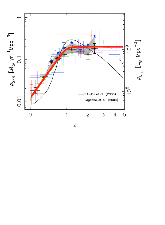
Figure 29: The observational data on the star formation rate as a function of redshift as compiled in SFRpaper . The thick (red) line is used in our calculations.

B.5 Spallation

Spallation –the production of secondary stable and unstable CRs by interactions of primaries with the ISM– is a well studied and fairly well understood phenomenon Silberberg . We do not discuss the subject further, since our theory does not significantly deviate from the standard lore on this subject.

B.6 Pion photoproduction

The intergalactic space is permeated by very low-density ionized gas, MFs, photons and neutrinos, and perhaps by other relics from the Big Bang and stellar evolution. The various ‘bands’ of the flux of photons of the CBR are shown in Fig 30 HD . The intergalactic medium is extremely transparent to CRs, except at very high energies. Greisen and Zatsepin & Kuzmin (GZK) were first to point out that the interactions of CR nuclei with the abundant but soft photons of the CMB would deplete the CR flux at energies above the pion-production threshold GZK . For nuclei of atomic number $A$ and energy:

$$E_{{}_{\rm GZK}}(A)\sim A\times 10^{20}\;\rm eV,$$ (99)

the energy loss length Stanev on the CBR is about half the size of the visible Universe, decreasing exponentially at higher energies.

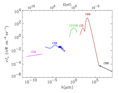
Figure 30: Illustration of the observed spectral flux of the CBR in the radio (CRB), microwave (CMB), infrared (CIB), optical-ultraviolet (CUVOB), X-ray (CXB) and $\gamma$-ray (CGB) bands HD .

The GZK effect introduces a sharp cutoff on the flux of UHECRs originating at large look-back times, as shown in Fig. 31. To an approximation sufficiently good for our purposes, we shall parametrize the effect of the GZK cutoff by a probability for the overall time-integrated flux of extragalactic nuclei to reach our Galaxy:

$$P_{\rm GZK}(E,A)=\exp\left[-\,{E\over E_{{}_{\rm GZK}}(A)}\right]\,.$$ (100)

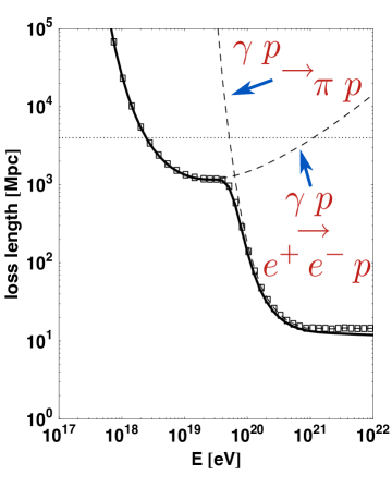
Figure 31: Solid line: loss length for pion and $e^{+}\,e^{-}$ photoproduction for CR protons on the CMB. The dashed lines are the separate contributions of the two processes. The dotted line shows the loss length for redshift losses Stanev .

B.7 Pair production

The production of $e^{+}e^{-}$ pairs in the interactions of extragalactic CR nuclei with the CBR also results in a reduction of the momentum of the former. The LF threshold for Bethe–Heitler pair production by CR nuclei on a CBR photon of energy $\epsilon_{\gamma}$ is almost the same for all $A$:

$$\gamma_{\rm pair}\geq{m_{e}\,c^{2}\over\epsilon_{\gamma}}\,\left[1+{m_{e}\over A\,m_{p}}\right].$$ (101)

The most abundant background radiation is the CBR, for which $\langle\epsilon_{\gamma}\rangle\simeq 0.63$ meV, and $\gamma_{\rm pair}\approx 8.1\times 10^{8}$, corresponding to $E\approx 7.6\times 10^{17}$ eV for protons. The cross section abruptly increases to $\sim 3/4$ of its constant high-energy value in a decade of energy and, not surprisingly, detailed calculations Stanev show that proton attenuation due to pair production on the CMB becomes important for energies around the ankle, at $3\times 10^{18}$ eV, as can be seen in Fig. 31.

De Marco and Stanev Stanev have made a systematic study of the effect of pair production and pion production on an extragalactic UHECR flux with various power source spectra $\propto E^{-\beta}$, including our predicted $\beta\simeq 2.5$. Their results can be very well reproduced by a multiplicative combination of the GZK cutoff of Eqs. (99), (100) and a factor describing pair production:

$$\!\!\!\!\!P_{\rm pair}(E)=1-0.55\,\exp\left\{-\,{\left[\log_{10}(E)-\log_{10}(E_{\rm pair})\right]^{2}\over\alpha}\right\}$$

$$E_{\rm pair}=8\times 10^{9},\;{\rm GeV}\;\;\;\;\;\;\alpha=1.4,$$ (102)

which we adopt as our description of the effect of pair production on the extragalactic proton flux.

The energy loss per pair-producing collision is ${\cal{O}}(2\,\gamma m_{e}\,c^{2})$ and the fractional energy loss is ${\cal{O}}(2\,m_{e}/A\,m_{p})$, i.e. $A$ times smaller for a nucleus than that for a proton. Since the pair-production cross section is proportional to $Z^{2},$ the energy-loss rate for nuclei is larger by a factor $Z^{2}/A$ than for protons. But, as we shall see in the next Section, photo-dissociation has a much larger effect on the fate of extragalactic nuclei than pair production has.

B.8 Photo-dissociation of nuclei

The main mechanism of energy loss by UHECR nuclei is photo-dissociation PSB in collisions with the photons of the CBR. The frequency interval most relevant to this process extends from the UV to the far infrared (FIR); the corresponding observations HD are summarized in Fig. 32. Let $dn_{\gamma}/d\epsilon$ be the number of CBR photons per unit energy $\epsilon$. Its relation to $\nu\,I_{\nu}$, plotted in Figs. 30,32, is:

$$\epsilon^{2}\,{dn_{\gamma}\over d\epsilon}\,[{\rm eV\,cm^{-3}}]=2.62\times 10^{-4}\,\nu\,I_{\nu}\,[{\rm nW\,m^{-2}\,sr^{-1}}].$$ (103)

Figure 32: Summary of extragalactic background radiation measurements in the ultraviolet (UV), visible, infrared and far infrared (FIR) HD . Square symbols and X’s are lower limits obtained by integrating resolved sources. Diamonds and triangles are, respectively, $1\sigma$ and $2\sigma$ upper limits obtained from fluctuation measurements. All other symbols show absolute background measurements. The shaded region represents the current uncertainty range of the CBR and the dotted line the present best estimate.

To introduce some relevant quantities, it is convenient to discuss first a steady-state Universe identical to the current one, and having existed for a Hubble time (in the current cosmology, the Hubble time, $\tau_{{}_{\rm H}}=9.8\times 10^{9}\,h^{-1}=15$ Gy, coincides to a very good approximation with the age of the Universe: $t_{{}_{\rm U}}\approx 0.96\,\tau_{{}_{\rm H}}$). The photo-disintegration rate PSB in the current-Universe’s ‘rest’ frame (in which the CMB is most isotropic) is:

$$R_{0}={c\over 2}\,\int_{\epsilon_{\rm th}\over 2\gamma}^{\infty}{d\epsilon\over\gamma^{2}\,\epsilon^{2}}\,{dn_{\gamma}\over d\epsilon}\int_{\epsilon_{\rm th}}^{2\gamma\epsilon}d\epsilon^{\prime}\,\epsilon^{\prime}\sigma(\epsilon^{\prime}),$$ (104)

where $\sigma$ is the total cross section, summed over the various nuclear break-up processes and $\epsilon_{\rm th}$ is the reaction’s energy threshold. At low energies the cross section is dominated by the giant dipole resonance which, in the nuclear rest frame, peaks at photon energies ranging from 10 to 30 MeV and has a width of ${\cal{O}}(10)$ MeV. The cross section obeys the approximate Thomas–Reiche–Kuhn sum rule:

$$\int_{\epsilon_{\rm th}}^{\infty}\sigma(\epsilon)\,d\epsilon={2\,\pi^{2}\,e^{2}\,\hbar\over m_{p}\,c}\,{N\,Z\over A}\approx 15\,A\,{\rm mb\,\,MeV},$$ (105)

where $N=A-Z$ is the neutron number, $\epsilon$ is the photon energy in the rest system of the nucleus and, in the last equality, $N\,Z/A$ has been approximated by $A/4$. Upon substitution of the sum rule in Eq. (104) we obtain:

$$R_{0}\approx{4.5\times 10^{-3}\,A\,{\rm cm^{3}\,eV^{2}\,s^{-1}}\over\gamma^{2}}\,\int_{\epsilon_{\gamma}}^{\infty}{d\epsilon\over\epsilon^{2}}\,{dn_{\gamma}\over d\epsilon},$$ (106)

where we have roughly approximated $\sigma$ by a peak at 15 MeV, so that $\epsilon_{\gamma}\approx 1.5\times 10^{7}\;{\rm eV}/\gamma$. We have explicitly checked that this is a good approximation, and so is the neglect of the fact that $\epsilon^{2}\,dn_{\gamma}/d\epsilon$ drops abruptly at frequencies beyond the UV.

The spectral energy density is roughly constant in the UV to FIR interval and has a value $\epsilon^{2}\,dn_{\gamma}/d\epsilon\sim 6\times 10^{-3}\,{\rm eV\,cm^{-3}}$, as can be seen in Fig. 32. Consequently, Eq. (104) yields a nuclear photo-dissociation rate:

$$R_{0}\approx 2.7\times 10^{-27}\,\gamma\,A\,{\rm s^{-1}},$$ (107)

The current mean photo-dissociation time coincides with $\tau_{{}_{\rm H}}$ when the energy of the CRs, independently of their $A$-value, is:

$$E_{\rm PhD}\simeq 7\times 10^{17}\;\,\rm eV,$$ (108)

or with $\sim\tau_{{}_{\rm H}}/5$ when $E=E[{\rm ankle}].$ In the fake steady-state Universe, the flux of CRs generated at look-back time $t$ is depleted as:

$$-{dn\over n}=R_{0}\,dt\approx{E\over E_{\rm PhD}}\,{dt\over\tau_{H}}\;,$$ (109)

and the corresponding attenuation is $a(E,t)=\exp[-(E/E_{\rm PhD})\,(t/\tau_{{}_{\rm H}})]$.

To deal with our actual Universe we must paraphrase the above calculation for an expanding Universe in which the CR production rate and the amount of (accumulating, non-primordial) background radiation vary with time. The spectral index of UHECRs above the ankle, without any type of attenuation, is predicted to be $\beta\simeq 2.5$. Attenuated only by redshift and expansion in the standard Universe, such a flux maintains its spectral index, but is reduced in magnitude by an overall factor:

$$I_{\rm SU}\simeq H_{0}\,\int{R_{\rm SF}(z)\over R_{\rm SF}(0)}\,{dt\over dz}\,{dz\over(1+z)^{\beta-1}}\approx 3.15.$$ (110)

The time evolution of the spectral energy density in the UV to FIR range is:

$$\epsilon^{2}\,{dn_{\gamma}(z)\over d\epsilon}=(1+z)^{3}\,\int_{z}^{\infty}\epsilon^{\prime}\,\mathcal{L}_{\epsilon}(\epsilon^{\prime},z^{\prime}){dt\over dz^{\prime}}\,{dz^{\prime}\over 1+z^{\prime}}\,,$$ (111)

where $\mathcal{L}_{\epsilon}$ is the spectral luminosity density in a comoving unit volume at $\epsilon^{\prime}=(1+z^{\prime})\,\epsilon$. In the approximation of no spectral evolution of the luminosity sources and an evolution of their numbers described by the star formation rate, Eq. (111) can be rewritten as:

$$\epsilon^{2}\,{dn_{\gamma}(z)\over d\epsilon} \approx (1+z)^{3}\,\epsilon^{2}\,{dn_{\gamma}(0)\over d\epsilon}\;{F(z)\over F(0)},$$

$$F(z) \equiv \int_{z}^{\infty}{R_{\rm SF}(z^{\prime})\over R_{\rm SF}(0)}\,{dt\over dz^{\prime}}\,{dz^{\prime}\over(1+z^{\prime})}\,.$$ (112)

In analogy with Eq. (109), the attenuation of the flux of CRs observed at energy $E$ and generated at redshift $z$ satisfies:

$$-{dn\over n} = {E\over E_{\rm PhD}}\,H(z),$$

$$H(z) \equiv (1+z)^{4}\,{F(z)\over F(0)}\,{dz\over g(z)}\;,$$ (113)

where $F(z)$ is as in Eq. (112) for the past background radiation, and $g(z)$ is the function involved in the time–redshift relation, Eq. (93). The corresponding CR attenuation factor is:

$$a(z,E)\simeq\exp\left[-\,{E\over E_{\rm PhD}}\,\int_{0}^{z}H(z^{\prime})\,dz^{\prime}\right]\,.$$ (114)

Attenuated by this extra photo-dissociation factor, the reduction factor of Eq. (110) becomes:

$$I_{\rm PhD}[E]=H_{0}\,\int a(z,E)\,{R_{\rm SF}(z)\over R_{\rm SF}(0)}\,{dt\over dz}\,{dz\over(1+z)^{\beta-1}}.$$ (115)

The attenuation of the flux of UHECR nuclei due exclusively to photo-dissociation is given by the $A$-independent ratio ${A}_{\rm PhD}(E)=I_{\rm PhD}[E]/I_{\rm SU}$. The actual result of the calculation of Eqs. (110) to (115) is well described by:

$${A}_{\rm PhD}(E)\approx{1\over\sqrt{1+(I_{\rm SU}\,E/E_{\rm PhD})^{2}}}\,.$$ (116)

This result is affected by the uncertainty in the current and past UV, visible and infrared CBR, but is otherwise a sufficiently good approximation for our purposes.

Photo-dissociation is a multiple-step process in which the debris eventually end up as protons and neutrons which $\beta$-decay to protons. Their individual energies are $\simeq 1/A$, the energy of the parent nucleus whose CR abundance has been enhanced by a factor $Z^{\beta_{\rm conf}}$ by CB acceleration. Consequently, a complete photo-dissociation of the UHECR nuclei would increase the proton flux by a factor $\Sigma_{Z}A[Z]\,X_{\rm SB}[Z]\,Z^{\beta_{\rm conf}}\simeq 1.6$.

At CR energies of order $E_{\rm PhD}$, photo-dissociation is not complete. The average reduction of the parent-nucleus atomic mass in a single photo-dissociation process at the relevant laboratory energies is observed to be $\Delta A\simeq 1.2$ for He, $\Delta A\simeq 3.6$ for the CNO group and, $\Delta A\simeq 3.7$ for elements ranging from Na to Fe. Consequently, He is efficiently photo-dissociated in a couple of steps at energies above $E_{\rm PhD}$, and we have simply treated the fraction of the He flux that is photo-dissociated as an addition to the proton flux:

$$\Delta F^{p}_{[{\rm He}\to p]}(E)\,dE^{p}=F^{\rm He}_{\rm PhD}(4\,E)\,dE^{\rm He},$$ (117)

where the $dE$ factors are reminders of the fact that it is baryon number which is conserved. Similarly, in $n(A)$ photo-dissociations, the heavier elements have their flux reduced by a factor

$$r\sim\left[{A-n(A)\,\Delta A\over A}\right]^{\beta-1}.$$ (118)

Only traces of relatively heavy fragments remain in the UHECR flux, since their ab-initio relative abundances are small. We have simply described the photo-dissociation of the corresponding primary fluxes by the substitution $E_{\rm PhD}\rightarrow n(A)\,E_{\rm PhD}$ in Eq. (116), with $n(A)=2$ for $A<8$, increasing linearly thereafter up to $n(A)=15$ at $A=56$. These values of $n(A)$ are estimates of the number of photo-dissociations required for the value of $r$ in Eq. (118) to represent a significant reduction (scaling up $E_{\rm PhD}$ by a factor $n(A)$ is tantamount to reducing the nuclear mean free path by the same amount).

Appendix C Jets in Astrophysics

A look at the sky, or a more economical one at the web, results in the realization that jets are emitted by many astrophysical systems: forming stars, binary stars, planetary nebulae, pulsars, radio galaxies, quasars, and microquasars. High-resolution radio, optical and X-ray observations indicate that (apparently ‘superluminal’) relativistic jets are fired by quasars, microquasars and SN explosions. These jets consist of a sequence of plasmoids (CBs) of ordinary matter whose initial expansion in their rest frame —presumably at a speed close to that of sound in a relativistic plasma— stops shortly after launch. One impressive instance WYS is that of the quasar Pictor A, shown in Fig. 2. Somehow, the active galactic nucleus of this object is discontinuously spitting something that does not appear to expand sideways before it stops and blows up, having by then travelled for a distance of several times the visible radius of a galaxy such as ours. Many such systems have been observed. They are very relativistic: the LFs of their ejecta are typically of ${\cal{O}}(10)$. The mechanism responsible for these mighty ejections —suspected to be due to episodes of violent accretion into a very massive black hole— is not understood.

Microquasars are binary systems consisting of a stellar-mass black hole or a neutron star accreting mass from a normal-star companion and displaying in miniature some of the main properties of quasars. The matter lost from the companion temporarily stations in a fast-spinning accretion disk, heated to millions of degrees. Aperiodically, a fraction of the disk falls towards the compact object, and a fraction of it is axially emitted as a pair of relativistic CBs. Some dozen microquasars have been found in the Milky Way. The first, GRS 1915+105, 40,000 light-years away in Aquila, was discovered in 1994 by the GRANAT X-ray satellite. It consists of a main-sequence star orbiting around the heaviest stellar black hole found to date, with a mass of $14\,M_{\odot}$. Already in its year of discovery, it was observed to shoot out, a few times a year, aperiodically, pairs of CBs with one-third the mass of the Moon and a $v\sim 0.92\,c$ Felix . Some properties of one of its CB-firing events are shown in Fig. 33.

Figure 33: Illustration of one side of a CB-shooting event in GRS 1925+105 Felix . The X-ray emission —attributed to an unstable accretion disk— temporarily decreases when the CBs are ejected DMR . How part of the accreting material ends up ejected along the system’s axis is not understood.

The continuous collision of CBs with the ISM produces in the latter turbulent magnetic fields, which gather and scatter the ionized ISM particles on their path. The collisions result in bremstrahlung, line emission and synchrotron radiation. Atomic lines from many elements have been observed in the optical Eiken and X-ray Kotani emission from the CBs of microquasar SS 433, indicating that the jetted ejecta are in this case —and reasonably in all cases— made of ordinary matter, and not of some fancier substance such as $e^{+}e^{-}$ pairs.

C.1 The motion of CBs

In analogy with the ‘hot-spots’ of quasars such as Pictor A, two infrared and radio sources appear symmetrically located with respect to GRS 1915+105, aligned with the position angle of the relativistic ejecta RM . They were presumably created by the plasmoids from GRS 1915+105, which finally stop and blow up nearly $60$ pc away from their ejection point. Even the mildly relativistic CBs from microquasars appear to travel a very long distance until their gradual deceleration in their interactions with the ISM finally stops them. In the case of XTE J1748–288 an originally ballistic jet was observed to stop over the course of a few weeks, presumably following a collision with denser environmental material kot00 .

In one case, that of XTE J1550–564, the gradual deceleration of CBs has been observed. A major radio-flare took place in September 1998. The resulting eastern CB was observed with Chandra between June 2000 and June 2002 Corbel , as shown in Figs. 34 and 35. The emission from the western CB was first detected on 11 September 2000 after it flared up. Probably this CB moved through a very low density region before it encountered a denser region and flared up.

Figure 34: Five Chandra 0.3–8 keV images showing the microquasar XTE J1550–564 and the evolution of the eastern and western X-ray emitting CBs between June 2000 and June 2002. The observations are ordered chronologically from top to bottom, and each image is labelled with the observation date. The dashed lines mark the positions of XTE J1550-564 and the eastern X-ray jet on 11 September 2000 Corbel .

Figure 35: The decelerating motion of the CBs of the $\mu$-quasar XTE J1550–564 Corbel .

C.2 CBs or conical jets?

The conical or trumpet-like radio and optical images of some astrophysical jets are often interpreted as being produced by conical ejecta. Conical-like images are often produced by precession of the ejection axis around the rotation axis, as in the case of SS433 Margon .

The conical flows that are produced along the motion of the decelerating CBs can also generate conical-looking trails. Radiation and charged particles (swept in ionized ISM particles), which are emitted isotropically in the CBs’ rest frame, are beamed forward by its motion.

Let primed quantities denote their values in the CB’s rest frame and unprimed quantities their corresponding values in the SN frame. The angle $\theta^{\prime}$ —relative to the CBs’ direction of motion— of the particles emitted in the CBs’ rest frame, and the corresponding angle $\theta$ in the SN’s rest frame, are related through:

$$\cos\theta^{\prime}={\cos\theta-\beta\over 1-\beta\,\cos\theta}\,.$$ (119)

Applied to an isotropic distribution of emitted particles in the CBs’ rest frame, Eq. (119) results in a distribution in the SN’s frame:

$${dn\over d\Omega}={dn\over d\Omega^{\prime}}\,{d\cos\theta^{\prime}\over d\cos\theta}\approx{n\over 4\,\pi}\,\delta^{2}\approx{n\over 4\,\pi}\,\left[{2\gamma\over 1+\gamma^{2}\,\theta^{2}}\right]^{2}\,,$$ (120)

where the Doppler factor $\delta$ of the CB’s radiation, as viewed from an angle $\theta$, was approximated by:

$$\delta={1\over\gamma\,(1-\beta\,\cos\theta)}\approx{2\gamma\over 1+\gamma^{2}\,\theta^{2}}\;,$$ (121)

which is well satisfied for CBs with $\gamma^{2}\gg 1\,,$ and $\theta^{2}\ll 1$. The ISM particles, which are isotropized elastically within the moving CB, are emitted with energy $\langle\epsilon\rangle=\gamma\,\delta\,m\,c^{2}.$ Hence, the energy outflow from a CB is:

$${dE\over d\Omega}={n\,m\,c^{2}\,\gamma\,\delta^{3}\over 4\,\pi}\,\approx{n\,\gamma\,m\,c^{2}\over 4\,\pi}\,\left[{2\,\gamma\over 1+\gamma^{2}\,\theta^{2}}\right]^{3}\,.$$ (122)

The distribution of the energy outflow from a decelerating CB is collimated into the narrow ‘beaming cone’ of Eq. (122), along the direction of motion of the CB. Subsequently the emitted charged particles are isotropized by the ambient MF and slowly diffuse away from the CBs’ trajectories. Most of the electrons’ energy is radiated via synchrotron emission in the MFs and inverse Compton scattering of CBR photons. This secondary radiation originates from outside the CB’s original beaming cone, diminishing with distance to the CBs’ trajectories: it may look like a much wider cone or domain. The narrow geometry of the relativistic ejecta reveals itself only in observations at much higher frequencies, the observed emission requiring much stronger MFs than those present in the ISM and IGM: the MFs within the CBs.

In our theory of GRBs and CRs, our Galaxy and its halo are at any point in time permeated by thousands of traveling CBs. Why have they not been observed? The answer is simple, and provided by Eq. (122). Their radiation at all wavelengths is tiny, except extremely close to their direction of motion: $\delta^{3}$ decreases dramatically at angles larger that $1/\gamma$, a few milliradians.

Appendix D More on the CB Model

The ‘cannon’ of the CB model is analogous to the ones responsible for the ejecta of quasars and microquasars. Long-duration GRBs, for instance, are produced in ordinary core-collapse SNe by jets of CBs, made of ordinary-matter plasma, and travelling with high LFs, $\gamma\sim{\cal{O}}(10^{3})$. An accretion disk or torus is produced around the newly born compact object, either by stellar material originally close to the surface of the imploding core and left behind by the explosion-generating outgoing shock, or by more distant stellar matter falling back after its passage ADR ; GRB1 ; DD . A CB is emitted, as observed in microquasars Felix ; DMR , when part of the accretion disk falls abruptly onto the compact object GRB1 ; DD .

Massive stars shed much of their matter in their late life, in the form of stellar ‘winds’. Even before they die as SNe, they undergo occasional explosions and rebrightenings, that illuminate their semi-transparent ‘wind-fed’ circumstellar material, creating a light echo, or ‘glory’. The example of the red supergiant V838 Monocerotis Bond is shown in the right panel of Fig. 36. As a SN explodes, it also illuminates its surroundings, producing a scattered, non-radially-directed ambient light that permeates the semi-transparent circumburst material, previously ionized by the early extreme UV flash accompanying the explosion, or by the enhanced UV emission that precedes it.

Figure 36: Left: Two relativistic CBs emitted in opposite directions by the microquasar XTE J1550-564, seen in X-rays Corbel . Right: HST picture from 28 October 2002 of the glory, or light echo, of the outburst of the red supergiant V838 Monocerotis in early January 2002 Bond . The light echo was formed by scattering off dust shells from previous ejections.

The $\gamma$-rays of a GRB are produced by inverse Compton scattering of the ambient light permeating the vicinity of the exploding star by the electrons enclosed in the CB. To produce, in the CB model, a GRB pulse by ICS of ambient light, it suffices to ‘superimpose the two halves’ of Fig. 36 Corbel ; Bond , and to work the result out in detail for the specific SN environment. The CBs electrons, comoving with it at a LF $\gamma\sim{\cal{O}}(10^{3})$, Compton up-scatter the ambient photons of energy $E_{i}$ to energies of ${\cal{O}}(\gamma^{2}\,E_{i})$, while beaming them forward at angles of ${\cal{O}}(1/\gamma)$. The collimated GRB is seen by a distant observer only when the jet points fairly precisely in her direction.

The time structure of GRBs ranges from a single pulse of $\gamma$-rays to a complicated succession or superposition of many pulses. A single pulse is generated as a CB coasts through the ambient light. The timing sequence of the successive individual pulses (or CBs) reflects the chaotic accretion process; its properties are not predictable, but those of the single pulses are.

Each pulse lasts from a fraction of a second to tens of seconds. The two-pulse $\gamma$-ray number count as a function of time for GRB 030329 is given, as an example, in Fig. 37, which also shows the CB-model description of its two pulses DDD329a . The CB-model predicts the properties of XRFs and long-duration GRBs remarkably well DD , as summarized in Appendix D.4 and briefly updated in Section X.1.

Figure 37: The $\gamma$-ray number count $dN/dt$ of GRB 030329, as measured by HETE II Vander , showing two dominant pulses, or CB contributions. The continuous line is the CB-model’s description of the line shapes DDD329a .

Long-duration GRBs have ‘afterglows’, long term emissions that are often observable at frequencies ranging from radio to X-rays, for months after their $\gamma$-rays are seen. The rapid expansion of the CBs stops shortly after ejection by their interaction with the ISM AGoptical . As a CB pierces the ISM with a roughly constant radius, its emission is dominated by synchrotron radiation from swept-in ISM electrons, which spiral in the CBs’ enclosed MF. This picture yields an excellent description of the entire AG phase and allows us to infer the parameters of CBs AGoptical ; AGradio , as discussed in Appendix D.6. These parameters and their distributions, employed as ‘priors’, can be used to predict the properties of the prompt $\gamma$-ray phase of GRBs DD , much as we use them here to predict the properties of CRs.

D.1 Do supernovae emit cannonballs?

Up to quite recently, there was only one case in which the data were good enough to tell: SN1987A, the core-collapse SN in the LMC, whose neutrino emission was detected TWOBANGS . Speckle interferometry measurements made 30 and 38 days after the explosion NP did show two relativistic CBs, emitted in opposite directions, as shown in Fig. 38. The apparent motion of the approaching CB is ‘superluminal’: it appears to have moved faster than light and further than the receding CB in the same time, even if their real speeds are comparable, $v\!\simeq\!c$.

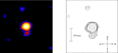
Figure 38: The two CBs emitted by SN1987A in opposite axial directions NP . The northern and southern bright spots are compatible with being jets of CBs emitted at the time of the SN explosion and travelling at a velocity equal, within errors, to that of light. One of the apparent velocities is superluminal. The corresponding GRBs were not pointing in our direction, which may have been a blessing.

Another resolved image of what appears like relativistic CBs emitted in a SN explosion was obtained recently with the Spitzer Space Telescope OK . Two FIR images of Cassiopeia A, the youngest observed SNR in our Galaxy (about 325 years old) show discrete compact structures at a distance of more than 20 arcmin from the SNR, moving in opposite directions at roughly the speed of light. The trail of the CBs inside and outside the SNR is still visible in an X-ray image of Cassiopeia A obtained by Chandra UH .

Cosmic GRBs are usually too far away to provide resolved (radio) images of CBs or their trails, except for relatively nearby GRBs such as GRB 980425, at $z=0.0085$ Galama and GRB030329, at $z=0.16$ Greiner . In the case of GRB 980425, the possibility was overlooked. The situation concerning GRB 030329 is debated. The supernova explosion SN2003dh that produced GRB 030329 was first detected spectroscopically on day 10 after the GRB SH , as predicted by the CB model DDD329a . The properties of its complex AG are also understood DDD329b . However, while we claim that the two CBs of this two-pulse GRB have been seen, in high-resolution radio observations, moving apart at an apparently superluminal velocity, at the predicted angular separation DDD329c , as shown in Fig. 39, the authors of the corresponding radio observations claim that their observed superluminal velocity does not agree with that predicted Taylor .

Figure 39: (a) The predicted angular displacement in the sky (in mas) of the two CBs of GRB 030329, as a function of observer’s time from the first day of radio observations, day $\sim 3$. The positions at day 0, the start-up time of the successive predicted rebrightenings of the slower CB1, the observed time of the intense late rebrightening of the faster CB2, as well as the fluences at 15.3 GHz on day 51 (70% and 30% of the total) are illustrated. The proper motion limit (PML) of Taylor et al. Taylor is also shown. (b) The expected angular distance between the two CBs as a function of time, and its measurement at day 51 Taylor .

D.2 Are GRBs made by SNe?

For long-duration GRBs, the answer is affirmative AGoptical ; DD ; AD2004 . The first spectroscopic evidence for a GRB–SN association came from the discovery of SN1998bw Galama , at redshift $z\!=\!0.0085$, within the directional error cone Soffitta towards GRB 980425. The time of the SN explosion was within $-\,2$ to $+\,0.7$ days of the GRB Iwamoto . The observations did not fit at all into the framework of the ‘standard’ fireball model. This GRB’s fluence was ‘normal’, but the total ‘equivalent isotropic’ $\gamma$-ray energy was $\sim\!10^{5}$ times smaller than that of ‘classical’ GRBs, with $z={\cal{O}}(1)$, transported to $z\!=\!0.0085$.

In the CB model the GRB emission is very narrowly forward-peaked, with a characteristic opening angle $\sim\!1/\gamma\!\sim\!1$ mrad along the opposite jets of CBs. Distant GRBs are only detectable if the observer is within an angle $\theta\!\sim\!1/\gamma$ relative to the emission axis. GRB 980425 was seen unusually far off-axis, its close location resulting in a ‘normal’ fluence. Its associated SN was seen unusually close to its axis of rotational symmetry. Both the GRB and the SN were otherwise fairly ‘normal’ AGoptical ; AGradio ; DD .

The optical luminosity of a 1998bw-like SN peaks at $\sim 15\,(1+z)$ days. The SN light competes at that time and frequency with the AG of its GRB, and it is not always easily detectable. In the CB model, it makes sense to test whether long-duration GRBs are associated with a ‘standard torch’ SN, akin to SN1998bw, ‘transported’ to their respective redshifts. The test works optimally: for all cases in which such a SN could be seen, it was seen (with varying degrees of significance) and for all cases in which the SN could not be seen, it was not seen; the redshift establishing in practice the transition to SN undetectability was $z\!\sim\!1.1$ AGoptical .

Naturally, truly ‘standard torches” do not exist, but SN1998bw made such a good job of it that it was possible to predict DDDSN ; DDD329a the SN contribution to the AG in all recent cases of early detection of the AGs of nearby GRBs (000911, 010921, 010405, 012111, 021211 and 030329). Besides the 980425–1998bw pair, the most convincing pre-Swift associations were provided by the spectroscopic discoveries of a SN in the AGs of GRBs 030329 SH and 021211 DV . For GRB 030329, shown in Fig. 40, even the exact date when the SN would be bright enough to be discovered was foretold DDD329a .

By now, the association between GRBs and core-collapse SNe (perhaps only of Types Ib,c) is fully established. The long history of this conclusion is reported in some detail in DDDNoSN .

Figure 40: Left: The R-band AG of GRB 030329, used along with other optical data to predict, in the CB model, the presence of a SN akin to SN1998bw. Right: The subsequent data (the $\star$ symbols) are added.

D.3 What fraction of SNe produce GRBs?

From a CB-model analysis of GRBs and their AGs AGoptical ; AGradio ; DDDSN ; DDD329a we conclude that GRBs more distant than GRB 980425 are observable, with past and current instruments, only for $\theta\leq$ 2–3 mrad. With two jets of very precisely collinear CBs per GRB, only a fraction

$$f\sim 2\,{\pi\,\theta^{2}/(4\,\pi)}\sim(2\;\rm{to}\;4.5)\times 10^{-6}$$ (123)

of SN-generated GRBs are observable.

The local rate of long-duration GRBs is estimated to be Schmidt $(2.5\pm 1.0)\times 10^{-10}\;{\rm Mpc^{-1}\,y^{-1}}$ for the current cosmology. The local rate of core-collapse SNe Capellaro is $(7.5\pm 3.8)\times 10^{-5}\;{\rm Mpc^{-1}\,y^{-1}}$. The ratio of these rates, $(3.3\pm 2.1)\times 10^{-6}$, is consistent with the fraction $f$ of observable GRBs. Thus, within the pervasive cosmological factor of a few, the long-GRB–SN association would be 1 to 1. Yet, the CBs of GRBs may not be emitted precisely in the same direction; a distribution of emission angles of a few mrad width, for instance, would not affect the results of the CB model, but would significantly increase $f$ in Eq. (123), diminishing the fraction of GRB-generating SNe. Current data are insufficient to determine whether long-duration GRBs are associated with all core-collapse SNe (some 70% of all SNe, including Type II) or only with Type Ib/c SNe (some 15% of all core-collapse SNe). Most well observed GRB-associated SNe are compatible with the latter of these possibilities.

Limits on the rate of SNe which produce GRBs, derived from wide-field deep surveys for radio-transient sources Levinson or in a targeted survey of optically selected SNe Ib/c Soderberg , have relied on the accepted but probably incorrect assumption Rhoads ; Sari ; Frail that the relativistic jets that produce GRBs are conical or trumpet-like in shape, stop shortly near their ejection site, and become an isotropic radio source, unlike in our discussion in Appendix C. As noted by Gal-Yam et al. Levinson , the limits are invalid, if the jets from SN explosions are similar to those fired by microquasars, as advocated by the CB model.

D.4 CB-model evidence for a SN–GRB association

Perhaps the best evidence that long-duration GRBs from SN explosions are produced by narrowly collimated relativistic jets, which are ejected in the explosion, comes from the remarkable success of the CB model in predicting the fluence, spectral and temporal properties of GRBs and of their AGs, despite their apparent complexity and large diversity.

For the GRB phase the CB-model consequences of a SN–GRB association —based exclusively on Compton scattering as the $\gamma$-ray-generating mechanism and on the hypothesis that the ‘windy’ material is less dense than average in the ‘polar’ directions— are essentially the list of properties of GRBs DD . To wit:

• The characteristic peak energy of the $\gamma$-rays: $E={\cal{O}}(250)$ keV, as observed by BATSE Preece and BeppoSAX Amati .

• The distribution of the ‘peak’ energies of the GRB spectra Preece .

• The duration of the single pulses of GRBs: a median $\Delta t\sim 1/2$ s FWHM McBreen .

• The typical (spherical equivalent) number of photons per pulse, $N_{\gamma}\sim 10^{59}$ on average, which, combined with the characteristic $\gamma$ energy, yields the average total (spherical equivalent) fluence of a pulse: $\sim 10^{53}$ erg DD .

• The general FRED pulse-shape: a very ‘fast rise’ followed by a fast decay $N(t)\propto 1/t^{2}$, inaccurately called ‘exponential decay’ Nemiroff ; McBreen .

• The $\gamma$-ray energy distribution, $dN/dE\sim E^{-\alpha}$, with, on average, $\alpha\sim 1$ exponentially evolving into $\alpha\sim 2.1$, and generally well fitted Band by the so-called ‘Band function”.

• The time–energy correlation of the pulses: the pulse duration decreases like $\sim E^{-0.4}$ and peaks earlier the higher the energy interval Fenimore .

• Various correlations between pairs of the following observables: photon fluence, energy fluence, peak intensity and luminosity, photon energy at peak intensity or luminosity, and pulse duration DD ; DDS05 .

• The possibly large polarization of the $\gamma$-rays Coburn .

In the CB model, X-ray flashes are simply GRBs viewed at larger angles, which makes their fluence and the energy of their quanta smaller, and their time structure less rugged DDDXRF . The recent progress in the understanding of GRBs and XRFs is discussed in Section X.1.

D.5 The “prompt” phase of a GRB or XRF

The distinction between a “prompt” and an “after”-glow phase —in terms of a given transition time— is arbitrary. Inverse Compton scattering dominates the early $\gamma$- and X-ray production, while synchrotron radiation (SR) from swept-in ISM electrons spiraling in the CB’s enclosed magnetic field dominates the X-ray signal at late times (the “late” $\gamma$-ray flux is too weak to be observable). For X-rays “prompt” and “ICS-dominated” are equivalent, and so are “afterglow” and “SR-dominated”. But at optical frequencies there are cases in which SR dominates during the “prompt” X-ray phase, and cases of ICS dominance in the X-ray “afterglow” phase. We summarize ICS in the this subsection, SR in the next.

The $\gamma$-rays of a single pulse of a GRB are produced as a CB coasts through the glory. The electrons enclosed in the CB boost the energy of the glory’s photons, via ICS, to $\gamma$-ray energies. The initial fast expansion of the CBs and the radially-increasing transparency of the windy environment result in the exponential rise of a GRB pulse. As a CB proceeds, the distribution of the glory’s light becomes more radially directed, its density decreases. Consequently, the energy of the observed photons is continuously shifted to lower energies as their number plummets. During a GRB pulse the spectrum softens and the peak energy decays with time, tending to a power law. This is also the behaviour of the X-ray “flares” of a GRB, which are either the low-energy tails of $\gamma$-ray pulses, or fainter and softer signals with the same origin.

The above effects can be explicitly analized DD , and summarized to a good approximation in a master formula for the temporal shape and spectral evolution of the energy fluence of an ICS-generated $\gamma$-ray pulse (or X-ray flare). For a single pulse starting at time $t=0$:

$$\!\!\!\!\!\!\!\!\!\!\!\!\!F_{E}\propto E\,{d^{2}N_{\gamma}\over dt\,dE}\propto$$

$$\!\!\!\!\!\!\!\!\!\!\!\!\!\Theta[t]\;e^{-[\Delta t/(t)]^{m}}\,\left\{1-e^{-[\Delta t/(t)]^{n}}\right\}\,E\,{dN_{\gamma}(E,t)\over dE}\;.$$ (124)

The time scale is set by $\Delta t$, with $\gamma\,\delta\,c\,\Delta t/(1+z)$ the radius of transparency of the glory, within which its photons are approximately isotropic. In $\Delta t$ time units, a pulse rises as ${\rm exp}[-1/t^{m}]$, $m\!\sim\!1$ to 2, and decreases as $1/t^{n}$, $n\!\sim\!2$. Finally, $E\,dN_{\gamma}/dE$ is the spectral function of the glory’s photons, up-scattered by the CB’s electrons, and discussed anon.

The glory has a thin thermal-bremsstrahlung spectrum: $E_{i}\,{dn_{\gamma}/dE_{i}}\!\sim\!(E_{i}/T_{i})^{1-\alpha_{g}}\,e^{-E_{i}/T_{i}}$, with a typical (pseudo)-temperature $T_{i}\!\sim\!1$ eV, and index $\alpha_{g}\!\sim\!1$. During the $\gamma$-ray phase of a GRB, the Lorentz factor $\gamma$ of a CB stays put at its initial value, for the deceleration induced by the collisions with the ISM has not yet had a significant effect. Let $\theta_{i}$ be the angle of incidence of the initial photon onto the CB, in the parent star’s rest system. The energy of an observed photon, Compton scattered in the glory by an electron comoving with a CB at redshift $z$, is given by $E\!=\!\gamma\,\delta\,E_{i}\,(1\!+\!\cos\theta_{i})/(1+z)$. The predicted GRB prompt spectrum is DD :

$$E\,{dN\over dE}\sim\left({E\over T}\right)^{1-\alpha_{g}}\,e^{-{E\over T}}+b\,(1-e^{-{E\over T}})\,\left({E\over T}\right)^{-{\beta_{\rm ac}\over 2}}.$$ (125)

The first term, with $\alpha_{g}\!\sim\!1$, is the result of ICS by the bulk of the CB’s electrons, which are comoving with it. The second term in is induced by a very small fraction of ‘knocked on’ and Fermi-accelerated electrons, whose initial spectrum (before Compton and synchrotron cooling) is $dN/dE_{e}\!\propto\!E_{e}^{-\beta_{\rm ac}}$, with an index assumed to be the same for electrons and nuclei, $\beta_{\rm ac}\!\approx\!2.2$, see Eq. (13). Finally, $T$ is the effective (pseudo)-temperature of the GRB’s photons, $T\!\equiv\!{4\,\gamma\,\delta\,T_{i}\,\langle 1\!+\!\cos\theta_{i}\rangle/[3\,(1+z)]}$. For a semi-transparent glory $\langle\cos\theta_{i}\rangle$ would be somewhat smaller than zero.

For $b={\cal{O}}(1)$, the energy spectrum predicted by the CB model, Eq. (125), bears a striking resemblance to the Band function Band traditionally used to model the energy spectra of GRBs Wigger . For many Swift GRBs the spectral observations do not extend to energies much bigger than $T$, or the value of $b$ in Eq. (125) is relatively small, so that the first term of the equation provides a very good approximation. At later times, the CB is sampling the glory at distances for which its light is becoming increasingly radial, $\langle 1\!+\!\cos\theta_{i}\rangle\!\to\!1/r^{2}\!\propto\!1/t^{2}$. For a pulse starting at $t\!=\!0$, the value of $E_{p}(t)$ consequently decreases as:

$$E_{p}(t)\approx E_{p}(0)\,\left[1-{t\over\sqrt{\Delta t^{2}+t^{2}}}\right]\,.$$ (126)

The light-curve of a single CB is well approximated by:

$$\!\!\!\!\!\!\!\!\!\!\!\!\!F_{E}\approx$$

$$\!\!\!\!\!\!\!\!\!\!\!\!\!\Theta[t]\;e^{-\left[{\Delta t\over t}\right]^{2}}\left\{1-e^{-\left[{\Delta t\over t}\right]^{2}}\right\}\left[{E\over E_{p}(t)}\right]^{1-\alpha_{g}}e^{-\left[{E\over E_{p}(t)}\right]}\,$$ (127)

until ICS is overtaken by synchrotron radiation. The generalization to a multi-pulse GRB is straightforward.

D.6 The Synchrotron Radiation “afterglow”

In the CB model, the AGs of GRBs and X-ray flashes (XRFs) consist of three contributions, from the CBs themselves, the concomitant SN, and the host galaxy:

$$F_{\rm AG}=F_{{}_{\rm CBs}}+F_{{}_{\rm SN}}+F_{{}_{\rm HG}}\,.$$ (128)

The latter contribution is usually determined by late-time observations, when the CB and SN contributions become negligible, or from measurements with sufficient angular resolution to tell apart $F_{{}_{\rm CBs}}+F_{{}_{\rm SN}}$ from $F_{{}_{\rm HG}}$.

The first convincing observation of a GRB–SN association was that of GRB 980425 with SN1998bw, at a record-low redshift $z_{bw}=0.0085$ Galama . In the CB model, we often used this SN as the ‘template’, or candidate ‘standard candle’ associated with GRBs. Let the unattenuated energy flux density of SN1998bw be $F_{bw}[\nu,t]$. For a similar SN placed at a redshift $z$ GRB1 ; AGoptical ; AD1999 :

$$F_{\rm SN}[\nu,t]={1+z\over 1+z_{bw}}\;{D_{L}^{2}(z_{bw})\over D_{L}^{2}(z)}\,A(\nu,z)\,F_{bw}[\nu^{\prime},t^{\prime}]\,,$$ (129)

where $A(\nu,z)$ is the attenuation along the line of sight, $\nu^{\prime}=\nu\,(1+z)/(1+z_{bw})$, and $t^{\prime}=t\,(1+z_{bw})/(1+z)$. The simple ansatz that all long-duration GRBs would be associated with SN1998bw-like SNe AD1999 ; DP ; GRB1 ; AGoptical proved to be unexpectedly precise and successful; see Appendix D.2.

The time dependence of $\gamma(t)$ —and, consequently, of the Doppler factor $\delta(t)$ of Eq. 121— is obtained from Eq. (11) and the relation between the observer’s time, $t$, and the travel-distance in the SN rest frame DD , $dx=c\,\gamma(t)\,\delta(t)\,dt/(1+z)$ [notice how $dx$ and $c\,dt$ may differ by a factor ranging up to ${\cal{O}}(10^{6})$]. Typically, within minutes of observer’s time, a CB reaches its roughly constant ‘coasting’ radius, $R_{0}\!=\!{\cal{O}}(10^{14}\,\rm cm)$, which increases slowly until the CB finally stops and blows up, as in Eq. (9). Up to the end of the coasting phase, and in a constant density ISM, $\gamma(t)$ obeys:

$$\!\!\!\!\!\!\!\!\!\!\!\!\!\!\!({\gamma_{0}/\gamma})^{4}+2\,\theta^{2}\,\gamma_{0}^{2}\,(\gamma_{0}/\gamma)^{2}=1+2\,\theta^{2}\,\gamma_{0}^{2}+t/t_{0}\,,$$

$$\!\!\!\!\!\!\!\!\!\!\!\!\!\!\!{t_{0}\over 1+z}={N_{{}_{\rm B}}\over 8\,c\,n_{p}\,\pi\,R_{0}^{2}\,\gamma_{0}^{3}}=$$

$$\!\!\!\!\!\!\!\!\!\!\!\!\!\!\!(1300\,{\rm s})\left[{10^{3}\over\gamma_{0}}\right]^{3}\,\left[{10^{-2}\,{\rm cm}^{-3}}\over n_{p}\right]\left[{10^{14}\,{\rm cm}\over R_{0}}\right]^{2}\left[{N_{{}_{\rm B}}\over 10^{50}}\right]$$ (130)

We have assumed that a CB’s magnetic field is in approximate energy equipartition with the energy of the intercepted ISM, $B\approx\sqrt{\pi\,n\,m_{p}\,c^{2}}\,\gamma$. In this field, the intercepted electrons emit synchrotron radiation. The SR, isotropic in the CB’s rest frame, has a characteristic frequency, $\nu_{b}(t)$, the typical frequency radiated by the electrons that enter a CB at time $t$ with a relative Lorentz factor $\gamma(t)$. In the observer’s frame:

$$\nu_{b}(t)\simeq{\nu_{0}\over 1+z}\,{[\gamma(t)]^{3}\,\delta(t)\over 10^{12}}\,\left[{n_{p}\over 10^{-2}\;\rm cm^{3}}\right]^{1/2}{\rm Hz}.$$ (131)

where $\nu_{0}\!\sim\!1.8\times 10^{16}\,\rm Hz\simeq 112\,eV$. The spectral energy density of the SR from a single CB at a luminosity distance $D_{L}$ is given by AGoptical ; AGradio :

$$\!\!\!\!\!\!\!\!\!\!\!\!F_{{}_{\rm CB}}\simeq{\eta\,\pi\,R_{0}^{2}\,n_{e}\,m_{e}\,c^{3}\,\gamma(t)^{2}\,\delta(t)^{4}\,A(\nu,t)\over 4\,\pi\,D_{L}^{2}}\,S(\nu,t)$$

$$\!\!\!\!\!\!\!\!\!\!\!\!S(\nu,t)\approx{1\over\nu_{b}(t)}\;{\beta_{\rm ac}-2\over\beta_{\rm ac}-1}\left[{\nu\over\nu_{b}(t)}\right]^{-{1\over 2}}\left[1+{\nu\over\nu_{b}(t)}\right]^{1-\beta_{\rm ac}\over 2}$$ (132)

where $\eta\!\approx\!1$ is the fraction of the impinging ISM electron energy that is synchrotron re-radiated by the CB, and $A(\nu,t)$ is the attenuation of photons of observed frequency $\nu$ along the line of sight through the CB, the host galaxy, the IGM and the Milky Way pfootnote .

At all times, X-rays are above the frequency $\nu_{b}$ in Eq. (131). It then follows from Eq. (132) that the unabsorbed X-ray spectral energy density has the form:

$$F_{{}_{\rm CB}} \propto R_{0}^{2}\,n_{e}^{(\beta_{\rm ac}+2)/4}\,\gamma^{(3\beta_{\rm ac}-2)/2}\,\delta^{(\beta_{\rm ac}+6)/2}\,\nu^{-\beta_{\rm ac}/2}$$ (133)

$$= R_{0}^{2}\,n_{e}^{\Gamma/2}\,\gamma^{3\,\Gamma-4}\,\delta^{\Gamma+2}\,\nu^{-\Gamma+1}\,,$$

where we used the customary notation $dN_{\gamma}/dE\!\approx\!E^{-\Gamma}$. Notice that the time evolution of the entire AG —via its $\gamma(t)$ and $\delta(t)$ dependences— is linked to its spectral behaviour. When testing this relation, which has a simpler asymptotic form discussed in the next paragraph, we fit the entire AG evolution in time DDDDecline .

The functions $\delta(t)/\delta_{0}$ and $\gamma(t)/\gamma_{0}$ evolve slowly, up until a time $t_{b}\!=\!(1+2\,\theta^{2}\,\gamma_{0}^{2})\,t_{0}$, with $t_{0}$ as in Eq. (130). The quantity $t_{b}$ characterizes the deceleration bend-time of the CB model; Eq. (130) for $\gamma(t,t_{0},\theta,\gamma_{0})$ describes the gradual character of this bend or ‘break’. At later times Eq. (130) implies that $\gamma\to\gamma_{0}\,(t/t_{0})^{-1/4}$, and Eq. (121) that $\delta\to 2\,\gamma$. Thus, at $t\!\gg\!t_{b}$, Eq. (133) yields:

$$F_{{}_{\rm CB}}(t) \propto t^{-1/2-\beta_{\rm ac}/2}\,\nu^{-\beta_{\rm ac}/2}=t^{-\Gamma+1/2}\,\nu^{-\Gamma+1},$$

$$\beta_{\rm ac} = 2\,(\Gamma-1),$$ (134)

with a predicted power decay in time half a unit steeper than in frequency, as long as the ISM has an approximately constant density. Density inhomogeneities complicate the shape of AGs. In an ISM with an approximate $1/r^{2}$ density profile, such as the galactic halos that CBs may reach late in their motion, the X-ray and optical time- and frequency- indices would differ by one unit, as opposed to one-half unit.

The prompt ultraviolet-to-infrared AG depends critically on the complex density profile along the CB’s trajectory and on the extinction along the line of sight. These complex environments can produce very bright and fast declining early-time AGs Akerlof ; DDDdens , or strongly extinct the early AG Rykoff , or even decelerate completely the CB, producing a ‘dark GRB’ Malessani .

In the radio, the AG spectrum is also affected by self-absorption in the CBs themselves, characterizable by one parameter per CB: a ‘free–free’ absorption frequency $\nu_{a}$ AGradio . At late time the radio emission from CR electrons ejected into the ISM along the CB trajectory can become important and even dominate the radio AG DDD329c .

We had previously posited and concluded DDD2003Lines ; DDDSwift that three mechanisms successively dominate the radiation of a GRB: ICS in the prompt phase, thermal bremsstrahlung and line emission in the fast-declining X-ray phase, SR thereafter. The line emission phase was supported by the claimed observations of X-ray lines in early GRB afterglows Xlines and their very natural CB-model interpretation DDD2003Lines . But these observations were of very limited statistical significance, and a phase during which line-emission significantly contributes may not, after all, be inevitably required.

The above description of GRB synchrotron radiation AGs is very simple and successful, and provides support to the CB model description of SN jets AGoptical ; AGradio ; DD ; DDD329b . We extract from the corresponding fits to the data the typical values of the CB parameters needed as inputs in our analysis of CRs and of the prompt $\gamma$-rays of GRBs. This is entirely analogous to what we did to predict the properties of the prompt ICS-dominated phase of a GRB from the parameters extracted from their AGs, and some other independent input “priors” DD .

Appendix E Short Hard GRBs

The origin of Short Hard Bursts (SHBs) is not established Nakar , in contrast to that of the longer-duration softer-spectrum GRBs. The SHB spectra and pulse-shapes are akin –except for hardness and duration– to those of long GRBs. The X-ray light curves of some well-sampled SHBs Burrows are ‘canonical’. The similarities suggest common mechanisms generating the GRB and SHB radiations. This is expected in the CB model, wherein both burst types are produced by jets of CBs Dar1995 . The ‘engine’ is different; it is a core-collapse SN for GRBs and XRFs, in SHBs it may be the result of mass accretion onto a compact object in a close binary system. In a SHB, the ambient light may be scattered by prior ejecta of the progenitor system (as in GRBs) or emitted by an accretion disc, or by the companion star.

In the CB model, the expressions that describe the promt and AG emissions of long GRBs are directly applicable to SHBs, provided the parameters of the CBs, of the glory, and of the circumburst environment, are replaced by those adequate for SHBs DDDSGRB .

The fluence of SHBs localized by Swift is 2 to 3 orders of magnitude smaller than for ordinary GRBs Berger . Their rate, measured (with different efficiency) by BATSE and the interplanetary network, is $20\%$ of the rate of long-duration GRBs. Assuming the same conversion efficiency of jet energy into $\gamma$-rays in SHBs and long GRBs, the CR luminosity produced by SHBs is also much smaller than that produced by core-collapse SNe.

Appendix F Power supply by other cosmic accelerators

Pulsars are born with typical periods of $P\gtrsim 30$ ms Lorimer . With a moment of inertia $I\sim 10^{45}\,{\rm gm\,cm^{2}}$ corresponding to a typical mass $\sim 1.4\,M_{\odot}$ and a radius $\sim 10$ km, their typical rotational energy is $E_{\rm rot}\simeq I\,\Omega^{2}/2=2\pi^{2}I/P^{2}\simeq 2\times 10^{49}$ erg. Most of this energy, which is two orders of magnitude smaller than the typical kinetic energy release in a core-collapse SN explosion, is radiated as magnetic dipole radiation and only a small fraction of it can be used to accelerate CR nuclei.

Soft Gamma-Ray Repeaters (SGRs) are slowly rotating ($P\sim$ 8–12 s), newly born pulsars which produce repeated ‘soft’ $\gamma$-ray bursts. Their rotational energy is too small to power either their persistent emission or their soft and hard $\gamma$-ray activity. Less than once in 30 years, they erupt in a hyperflare, such as that of the Galactic SGR 1806-20 on 27 December 2004, whose entire electromagnetic energy release was concentrated in a short spike of hard $\gamma$-rays that could have been interpreted as a normal SHB, had it taken place in an external galaxy within a distance of $\lesssim 30$ Mpc Hurley . But, if the hyperflare was relativistically beamed and was viewed slightly off axis, near-axis hyperflares from SGRs in external galaxies can be seen from much larger distances and may also be a source of SHBs DDDSGRB . As for SHBs in general, the contribution of SGRs to CRs would be negligible.

Neutron-star mergers (NSMs) are likely to produce relativistic jets which can be an origin of both SHBs GDN and UHECRs DLS . The estimated Galactic rate of NSMs Phinney is $\sim 1.8\times 10^{-4}\,{\rm y^{-1}}$, which is smaller than the Galactic SN rate by $\sim 2$ orders of magnitude; see Appendix B.3. Since, in addition, the kinetic energy of the jets that produce SHBs is smaller than for GRBs, the contribution of NSMs to the CR luminosity is negligible.

Microquasars fire mildly relativistic CBs. Power-law radio emission from their CBs provides evidence that they accelerate high-energy CR electrons Felix . Thus, microquasars were suggested as sources of relativistic CRs HS . But the total kinetic power of the jets of a dozen or so microquasars in our Galaxy Felix ; Kaaret is smaller than that of SN jets by 2 to 3 orders of magnitude, consistent with estimates HS of their relative contribution to the Galactic CR luminosity.

References

- (1) For recent reviews, see for instance, D.F. Torres & L.A. Anchordoqui, Rep. Prog. Phys. 67, 1663 (2004); A.A. Watson, astro-ph/0410514; J.W. Cronin, Nucl. Phys. B Proc. Suppl. 138, 465 (2005); A. Olinto, AIP Conf. Proc. 745, 48 (2005); J.R. Hoerandel, Nuovo Cim. B120, 825 (2005). R. Engel, Nucl. Phys. B (Proc. Suppl.) 151, 437 (2006). J.R. Hoerandel, astro-ph/0508014.
- (2) K.H. Kampert et al., Acta Phys. Polon. B35, 1799 (2004).
- (3) A. Zech et al., Nucl. Phys. B Proc. Suppl. 136, 34 (2004).
- (4) S. Haino et al., Phys. Lett. B594, 35 (2004).
- (5) V.L. Ginzburg & V.S. Ptuskin, Rev. Mod. Phys. 48, 161, (1976) and references therein.
- (6) G. Cocconi, Nuovo Cimento, 3, 1433 (1956).
- (7) P. Morrison, Rev. Mod. Phys. 29, 235 (1957).
- (8) R.U. Abbasi et al., Astrophys. J. 610, L73 (2004); S. Westerhoff et al., Nucl. Phys. B Proc. Suppl. 136C, 46 (2004).
- (9) The Pierre Auger Collaboration, Science 318, 938 (2007).
- (10) R. Plaga, astro-ph/0111555 and New Astronomy 7, 317 (2002). I.A. Grenier & P. Laurent Europhysics News, 32, 218 (2001).
- (11) See A.M. Hillas, J. Phys. G Nucl. Phys. 31, 39 (2005), for a recent review.
- (12) P. Nisenson & C. Papaliolios, Astrophys. J. 518, L29 (1999).
- (13) U. Hwang et al., Astrophys. J. 615, L117 (2004).
- (14) O. Krause et al., Science 308, 1604 (2005).
- (15) R.N. Manchester, Astron. & Astrophys. 171, 205 (1987).
- (16) A. Dar & R. Plaga, Astron. & Astrophys. 349, 259 (1999).
- (17) A. Dar, Nuovo Cim. B120, 767 (2005); A. De Rújula, Nucl. Phys. B (Proc. Suppl.) 151, 23 (2006).
- (18) A. De Rújula, Int. J. Mod. Phys. A20, 6562 (2005).
- (19) The association between high-energy CRs and GRBs was suggested by A. Dar, B. Kozlovsky, S. Nussinov & R. Ramaty [Astrophys. J. 388, 164, (1992)]. E. Waxman [Phys. Rev. Lett. 75, 386 (1995)], M. Milgrom & V. Usov [Astrophys. J. 449, 37 (1995)] and M. Vietri [Astrophys. J. 453, 883 (1995)] suggested that extragalactic relativistic fireballs, which allegedly produce GRBs, are the source of the UHECRs. A. Dar & R. Plaga DP maintained that SN explosions produce relativistic jets which are the main source of CRs at all energies and the source of narrowly beamed GRBs [N. Shaviv & A. Dar Astrophys. J. 447, 863 (1995)] and of GRB AGs [A. Dar, astro-ph/9704187 and Astrophys. J. 500, L93 (1998)], most of which do not point in our direction. C.D. Dermer [ Astrophys. J. 574, 65 (2002)] and S.D. Wick, C.D. Dermer & A. Atoyan [Astropart. Phys. 21, 125 (2004)] posit that GRBs are the main source of CRs only at eV.
- (20) A. Dar & A. De Rújula, astro-ph/0008474.
- (21) A. Dar & A. De Rújula, Phys. Rept. 405, 203, (2004).
- (22) P. Grandi et al., Astrophys. J. 586, 123 (2003).
- (23) A.S. Wilson, A.J. Young & P.L. Shopbell, Astrophys. J. 547, 740 (2001).
- (24) See, e.g. S.P. Swordy et al., Astrophys. J. 349, 625 (1990).
- (25) A. Dar, A. De Rújula & N. Antoniou, Proc. Vulcano Workshop 1999 (eds. F. Giovanelli and G. Mannocchi) p. 51 Italian Physical Society, Bologna-Italy, [astro-ph/9901004].
- (26) A. Dar & A. De Rújula, Mon. Not. Roy. Astr. Soc. 323, 391 (2001).
- (27) K. Greisen, Phys. Rev. Lett. 16, 748, (1966); G.T. Zatsepin & V.A. Kuzmin, JETP Lett. 4, 78 (1966).
- (28) M. Takeda et al., Phys. Rev. Lett. 81, 1163 (1998) and Astropart. Phys. 19, 447 (2003).
- (29) J.R.T. de Mello Neto et al., arXiv:0712.3727.
- (30) M. Unger et al., arXiv:0706.1495.
- (31) The distinction between parameters and priors has become established in the analysis of the CMB.
- (32) S. Dado, A. Dar & A. De Rújula, Astron. & Astrophys. 388, 1079 (2002).
- (33) S. Dado, A. Dar & A. De Rújula, Astron. & Astrophys. 401, 243 (2003).
- (34) S. Dado, A. Dar & A. De Rújula, Astron. &Astrophys. 422, 381 (2004).
- (35) A. Dar & A. De Rújula, Phys. Rev. D72, 123002 (2005).
- (36) S. Colafrancesco, A. Dar & A. De Rújula, Astron. & Astrophys. 413, 441 (2004).
- (37) A. De Rújula, Phys. Lett. B193, 514 (1987).
- (38) I.F. Mirabel & L.F. Rodriguez, Annu. Rev. Astron. Astrophys. 37, 409 (1999).
- (39) V. Dhawan, I. F. Mirabel & L.F. Rodriguez, Astrophys. J. 543, 373 (2000).
- (40) S. Dado, A. Dar & A. De Rújula, Astrophys. J. 646 L21 (2006).
- (41) There is no confirmed deviation from isotropy above the ankle, e.g. HIRES2 , or above the knee, e.g. T. Antoni et al. [Astrophys. J. 604, 687 (2004)] and any anisotropies at lower energies are very small. See e.g. A.G.K.Smith & R.W. Clay [Aust. J. Phys. 50, 827 (1997)] and R.W. Clay, M.A. McDonough & A.G.K. Smith [Publ. Astron. Soc. Aust. 15, 208 (1998)].
- (42) J.K. Frederiksen et al., Astrophys. J. 608, L13 (2004).
- (43) F. Quilligan et al., Astron. & Astrophys. 385, 377 (2002).
- (44) A.W. Strong & A.V. Moskalenko, Proc. 27th Int. Cosmic-Ray Conf. (Hamburg) p. 1964 (2001); A. W. Strong, I. V. Moskalenko, & O. Reimer, Astrophys. J. 613, 962 (2004).
- (45) M.S. Longair, High Energy Astrophysics (Cambridge University Press, 1992), and references therein.
- (46) V.A. Dogiel, V. Schönfelder & A.W. Strong, Astrophys. J. 572, L157 (2002).
- (47) D.E. Groom et al., Review of Particle Physics, Eur. Phys. J. C15, 1-878 (2000), p. 166.
- (48) A turbulent Kolmogoroff spectrum of magnetic inhomogeneities yields while a Kraichnan spectrum yields ; see V.S. Ptuskin et al. [Adv. Sp. Res. 35, 162 (2005)] and references therein.
- (49) J.J. Connell, Astrophys. J. 501, 59 (1998); J.J. Connell, Sp. Sci. Rev. 99, 41 (2001).
- (50) W.I. Axford, Proc. Int. Cosmic Ray Conf. (Paris), 12, 155 (1981).
- (51) J.C. Higdon & R.E. Lingenfelter, Astrophys. J. 628, 738 (2005) and references therein.
- (52) M. Miceli et al., astro-ph/0602518.
- (53) B. Wiebel-Sooth, P. Bierman & H. Meyer, Astron. & Astrophys. 330, 37 (1998).
- (54) N. Grevesse & A.J. Sauval, 1998, Sp. Sci. Rev. 85, 161 (1998); N. Grevesse & A.J. Sauval, Adv. Sp. Res. 30, 3, (2002).
- (55) M. Aguilar et al., Phys. Rep. 366, 331 (2002).
- (56) J.R. Hoerandel, Proc.“Workshop on Physics of the End of the Galactic Cosmic Ray Spectrum”, Aspen, USA, 2005 [astro-ph/0508014].
- (57) R. Wijmans, Astropart. Phys. 19, 379 (2003).
- (58) M. Zha, J. Knapp & S. Ostapchenko, Proc. 28th Int. Cos. Ray Conf. (Tsukuba), ICRC 2, 515 (2003).
- (59) R. Beck, Space Science Reviews, 99, 243 (2001).
- (60) S. Dado, A. Dar & A. De Rújula, Nuc. Phys. B165, 103 (2007).
- (61) A. W. Strong, I. V. Moskalenko & O. Reimer, Astrophys. J. 613, 962 (2004).
- (62) A. Dar & A. De Rújula, Astrophys. J. 547, L33 (2001).
- (63) B. Wiebel-Soth et al., Astron. & Astrophys. 330, 389 (1998).
- (64) J.R. Hoerandel, Astropart. Phys. 19, 193 (2003).
- (65) V.L. Ginzburg & S.I. Syrovatskii, Origin of cosmic rays The Macmillan Pub. Co. New York 1964.
- (66) J.C. Mather et al., Astrophys. J. 432, L15, (1993). D.J. Fixsen et al., Astrophys. J. 473, 576 (1996).
- (67) M. Sapinski et al., Proc. 29th International Cosmic Ray Conference, Pune, India, 101106 (2005).
- (68) P. Sreekumar et al., Astrophys. J. 494, 523 (1998), and references therein.
- (69) D.J. Thompson & C.E. Fichtel, Astron. & Astrophys. 109, 352 (1982).
- (70) J.E. Felten & P. Morrison, Astrophys. J. 146, 686 (1996).
- (71) N. Duric, J. Irwin & H. Bloemen, Astron. Astrophys. 331, 428 (1998).
- (72) A. Dar & N. J. Shaviv, Phys. Rev. Lett. 75, 3052 (1995).
- (73) M.H. Salamon & F.W. Stecker, Astrophys. J. 493, 547 (1998).
- (74) P.P. Kronberg et al., Astrophys. J. 604, 77 (2004).
- (75) Q. Yu and S. Tremaine, Mon. Not. Roy. Ast. Soc. 335, 965 (2002).
- (76) G. Bignami et al., Astrophys. J. 232, 649 (1979); D. Kazanas & J.P. Protheroe, Nature, 302, 228 (1983); F.W. Stecker & M.H. Salamon, Astrophys. J. 464, 600 (1996).
- (77) J. Chiang & R. Mukherjee, Astrophys. J. 496, 772 (1998).
- (78) R. Mukherjee & J. Chiang, Astropart. Phys. 11, 213 (1999).
- (79) http://heasarc.nasa.gov/docs/swift/swiftsc.html
- (80) The HIRES collaboration, arXiv:astro-ph/0703099.
- (81) M. Amenomori et al., arXiv:0801.1803.
- (82) M. Amenomori et al., Phys. Lett. B632, 58 (2006).
- (83) M. Ribó, Chinese Jour. of Astron & Astrophys (in press) (arXiv:0801.2906) .
- (84) A. Dar & A. De Rújula, astro-ph/0012227.
- (85) S. Dado, A. Dar & A. De Rújula, Astrophysical J. 663, 400 (2007).
- (86) S. Dado, A. Dar & A. De Rújula, arXiv:0712.1527
- (87) S. Dado, A. Dar & A. De Rújula, arXiv:0709.4307
- (88) S. Dado, A. Dar & A. De Rújula, arXiv:0706.0880
- (89) A. De Rújula, arXiv:0801.0397
- (90) M.P. Véron-Cetty & P. Véron, Astron. & Astrophys. 455, 773 (2006).
- (91) S. G. Jorstad et al., Astron. J. 130, 1418 (2005) and references therein.
- (92) R. Scarpa & C. M. Urry, New Astronomy Revs. 46, 405 (2002).
- (93) D. N. Spergel et al., The Astrophs. Jour. Suppl. 148, 175 (2003).
- (94) J.P. Rachen & P. L. Biermann, Astron. & Astroph., bf 272, 161 (1993).
- (95) G. Pulhoefer et al., Astroparticle Physics, 20, 267 (2003).
- (96) K. Koyama et al., Nature 378, 255 (1995).
- (97) S. Hoppe, for the HESS Collaboration, arXiv:0710.3528.
- (98) F. Aharonian et al., arXiv:astro-ph/0510397.
- (99) L. O. Drury, et al. Space Science Reviews, 99, 329 (2001).
- (100) D. C. Ellison, A. Decourchelle & J. Ballet, Astron. & Astrophys. 413, 2004; J. P. Hughes, C. E. Rakowski & A. Decourchelle, The Astrophys. Jour. 543, L61 (2000).
- (101) N. Panagia,, et al. Astrophys. J. 646, 369 (2006) and references therein.
- (102) F. Aharonian et al., Nature 432, 75 (2004).
- (103) F. Aharonian et al., Astron. & Astroph. 437, 135 (2005).
- (104) F. Aharonian et al., Astrophys. J. 636, 777 (2006).
- (105) J. Albert et al., Astrophys. J. 664, L87 (2007).
- (106) S. Dado & A. Dar, Astrophys. J. 627, L109 (2005).
- (107) http://swift.gsfc.nasa.gov/docs/swift/archive/ grb-table.html/
- (108) A. Dar, Phys. Rev. Lett. 51, 227 (1983).
- (109) A. Dar & A. De Rújula, arXiv:hep-ph/0611369.
- (110) F. W. Stecker & O. C. de Jager, Astroph. J. 476, 712 (1997).
- (111) R. Engel, D. Seckel & T. Stanev, Phys. Rev. D64, 093010 (2001).
- (112) F. Halzen, Eur. Phys. J. C46, 669 (2006).
- (113) S. Schindler, B. Binggeli & H. Bohringer, Astron. & Astroph., 343, 20 (1999).
- (114) W. Baade, & F. Zwicky, Proc. Nat. Acad. Sci. USA, 20/5, 259 (1934).
- (115) See, e.g., N.J. Shaviv, New Astron. 8, 39 (2002) and Phys. Rev. Lett. 89, 051102 (2002).
- (116) S. van den Bergh & G. A. Tammann, Annu. Rev. Astron. Astrophys. 29, 363 (1991).
- (117) C.J. Pritchet & S. van den Bergh, Astron. J. 118, 883 (1999).
- (118) R.S. Ellis, Annu. Rev. Astron. Astrophys. 35, 389 (1997).
- (119) P.G. Perez-Gonzalez et al., Astrophys. J. 630 82 (2005). D. Schiminovich et al., Astrophys. J. 619, L47 (2005) and references therein.
- (120) R. Silberberg & C.H. Tsao, Phys. Rep. 191, 351 (1990).
- (121) M.G. Hauser & E. Dwek, Annu. Rev. Astron. Astrophys. 39, 249 (2001) and references therein.
- (122) V.S. Berezinsky, A.Z. Gazizov & S.I. Grigorieva, Phys. Lett. B612, 147 (2005); D. De Marco & T. Stanev, Phys. Rev. D72, 081301 (2005) E. Khan et al. Astropart. Phys. 23, 191 (2005) and references therein.
- (123) W. Tkaczyk, J. Wdowczyk & A.W. Wolfendale, J. Phys. A. 8 1518 (1975); J.L. Puget, F.W. Stecker & J.H. Bredekamp, Astrophys. J. 205, 638 (205); S. Karakula & W. Tkaczyk, Astropart. Phys. 1, 229 (1993); F.W. Stecker & M.H. Salomon, Astrophys. J. 512, 521 (1999); L.N. Epele & E. Roulet, JHEP 9810, 9 (1998); J. Candia, L.N. Epele & E. Roulet, Astropart. Phys. 17, 23 (2002); E. Khan et al., Astropar. Phys. 23, 191 (2005).
- (124) S.S. Eikenberry et al., Astrophys. J. 561, 1027 (2001); D.R. Gies et al., Astrophys. J. 566, 1069 (2001).
- (125) M.G. Watson et al., Mon. Not. Roy. Astron. Soc. 222, 261 (1986); T. Kotani et al., Publ. Astron. Soc. Jap. 48, 619 (1996); H.L. Marshall, C.R. Canizares & N.S. Schulz, Astrophys. J. 564, 941 (2002); S. Migliari, R. Fender & M. Méndez, Science 297, 1673 (2002); M. Namiki et al., Publ. Astron. Soc. Jap. 55, 1 (2003).
- (126) L.F. Rodriguez & I.F Mirabel, New Astron. Rev. 42, 649 (1998).
- (127) T. Kotani et al., Astrophys. J. 543, L133 (2000).
- (128) S. Corbel et al., New Astron. Rev. 47, 477 (2003).
- (129) B. Margon, Annu. Rev. Astron. Astrophys. 22, 507 (1984).
- (130) H.E. Bond et al., Nature 422, 425 (2003).
- (131) R. Vanderspek et al., 2003, http://space.mit.edu/ HETE/Bursts/GRB030329.
- (132) S. Dado, A. Dar & A. De Rújula, Astrophys. J. 594, L89 (2003).
- (133) It was argued in Ref. ADR that the alleged two neutrino bursts of SN 1987A were due to the formation of a neutron star, followed by an accretion-induced collapse into a black hole. The idea would have been better accepted nowadays than it was at the time.
- (134) T. J. Galama et al., Nature 395, 670 (1998).
- (135) J. Greiner et al., GCN Circ. 2020 (2003).
- (136) K.Z. Stanek et al., Astrophys. J. 591, L17 (2003); J. Hjorth et al., Nature 423, 847 (2003).
- (137) S. Dado, A. Dar & A. De Rújula, astro-ph/0402374.
- (138) S. Dado, A. Dar & A. De Rújula, astro-ph/0406325.
- (139) G.B. Taylor et al., Astrophys. J. 622, 986 (2005).
- (140) A. Dar, astro-ph/0405386.
- (141) P. Soffitta et al., IAU Circ. 6884 (1998).
- (142) K. Iwamoto et al., Nature 395, 672 (1998).
- (143) S. Dado, A. Dar & A. De Rújula, Astrophys. J. 572, L143 (2002); S. Dado, A. Dar & A. De Rújula, Astron. & Astrophys. 393, L25 (2002); S. Dado, A. Dar & A. De Rújula, Astrophys. J. 593, 961 (2003).
- (144) S. Dado, A. Dar & A. De Rújula, arXiv:astro-ph/0611161.
- (145) M. Della Valle et al., Astron. & Astrophys. 406, L33 (2003).
- (146) M. Schmidt, Astrophys. J. 559, L79 (2001).
- (147) E. Capellaro, in Supernovae and GRBs, ed. K. W. Weiler (Springer, Berlin, 2003), p. 37.
- (148) A. Levinson et al., Astrophys. J. 576, 923 (2002); A. Gal-Yam et al., Astrophys. J. 639, 331 (2006). The comment in Frail also applies here and to Soderberg .
- (149) A.M. Soderberg, D.A. Frail & M.H. Wieringa, Astrophys. J. 607, L1 (2004).
- (150) J. E. Rhoads, Astrophys. J. 525, 737 (1999).
- (151) R. Sari, T. Piran & J.P. Halpern, Astrophys. J. 519, L17 (1999).
- (152) For a small opening angle, a conical GRB lights up a fraction of the full celestial sphere, or a fraction if is defined to be half the opening angle of the cone. The relation has been widely used by D.A. Frail et al. [Astrophys. J. 562, L55 (2001)] and by many other authors in their estimates of the true -ray energy of GRBs from the ‘Frail relation’, , where is the equivalent isotropic energy of the GRB deduced from its redshift and its measured fluence. The fraction of the full celestial sphere lighted up by two opposite conical GRBs, each of half opening angle , is and it should be used for estimating under the fireball-model assumption that two identical conical GRBs are emitted simultaneously in opposite directions.
- (153) R.D. Preece et al., Astrophys. J. Suppl. 126, 19 (2000).
- (154) L. Amati et al., Astron. & Astrophys. 390, 81 (2002).
- (155) S. McBreen et al., AIP Conf. Proc. 662, 280 (2003).
- (156) R.J. Nemiroff et al., Astrophys. J. 414, 36 (1993); R.J. Nemiroff, AIP Conf. Proc. 307, 7300 (1994); B. Link & R.I. Epstein, Astrophys. J. 466, 764 (1996).
- (157) D. Band et al., Astrophys. J. 413, 281 (1993).
- (158) E.E. Fenimore et al., Astrophys. J. 448, L101 (1995); J.P. Norris et al., Astrophys. J. 459, 393 (1996); B. Wu & E.E. Fenimore, Astrophys. J. 535, L29 (2000); E. Ramirez-Ruiz & E.E. Fenimore, Astrophys. J. 539, 12 (2000).
- (159) W. Coburn & S.E. Boggs, Nature 423, 415 (2003); D. R. Willis et al., Astron. & Astrophys. 439, 245 (2005); E. Kalemci et al., Astrophys. J. (Suppl.) 169, 75 (2007).
- (160) In cases where it is possible to distinguish between the phenomenological ‘Band’ spectrum and that predicted by the CB model, the latter provides a better fit, see C. Wigger et al., Astrophys. J. .675, 553 (2008).
- (161) A. Dar, Astron. & Astrophys. Suppl. 138, 505 (1999).
- (162) The normalization in Eq. (131) is only correct for , for otherwise the norm diverges. The cutoffs for the distribution are time-dependent, dictated by the acceleration and SR times of electrons and their ‘Larmor’ limit. The discussion of these processes being complex, we satisfy ourselves here with the statement that for the AG’s normalization is not predicted.
- (163) S. Dado, A. Dar, & A. De Rújula, Astrophys. J. 585, 890 (2003).
- (164) L. Piro et al., Astron. & Astrophys. 331, L41 (1998); A. Yoshida et al., Astron. & Astrophys. Suppl. 138, 433 (1999); A. Yoshida, et al., Astrophys. J. 557, L27 (2001); L. Piro et al., Science, 290, 955 (2000); L.A. Antonelli et al., Astrophys. J. 545, L39 (2000); J.N. Reeves et al., Nature, 416, 512 (2002); D. Watson et al., Astrophys. J. 595, L29 (2003).
- (165) C. Akerlof et al., Nature 398, 400 (1999).
- (166) S. Dado, A. Dar & A. De Rújula, Astrophys. J. 585, L15 (2003).
- (167) E. S. Rykoff et al., Astrophys. J. 601, 1013 (2004) and 631, L121 (2005).
- (168) D. Malesani et al., Nuovo Cim. 28C, 515 (2005).
- (169) For a review, see E. Nakar, Phys. Rep. 442, 166 (2007).
- (170) D.N. Burrows et al., Astrophys. J. 653, 468 (2006).
- (171) S. Dado, A. Dar & A. De Rújula, in preparation.
- (172) E. Berger et al., Nature 438, 988 (2005).
- (173) D.R. Lorimer, astro-ph/0301327.
- (174) A. Dar, GCN Circ. 2942 (2004); K. Hurley et al., Nature 434, 1098 (2005).
- (175) J. Goodman, A. Dar & S. Nussinov, Astrophys. J. 314, L7 (1987).
- (176) A. Dar, A. Laor & N.J. Shaviv, Phys. Rev. Lett. 80, 5813 (1998).
- (177) V. Kalogera et al., Astrophys. J. 601, L179 (2004); E.S. Phinney, Astrophys. J. 380, L17 (1991).
- (178) S. Heinz & R. Sunyaev, Astron. & Astrophys. 390, 751 (2002).
- (179) P. Kaaret et al., Nucl. Phys. B (Proc. Suppl.) 132, 354 (2004).