Abstract

We compute the next-to-leading order strong interaction corrections to gluino-mediated $\Delta F=2$ box diagrams in the Minimal Supersymmetric Standard Model. These corrections are given by two loop diagrams which we have calculated in three different regularization schemes in the mass insertion approximation. We obtain the next-to-leading order Wilson coefficients of the $\Delta F=2$ effective Hamiltonian relevant for neutral meson mixings. We find that the matching scale uncertainty is largely reduced at the next-to-leading order, typically from about 10-15% to few percent.

1 Introduction

If ongoing and planned experiments discover direct or indirect departures from the Standard Model (SM), the next step will be to understand what kind of new physics is involved. Detailed predictions for flavour changing neutral currents processes in supersymmetry play a crucial role in this program. In particular, flavour mixing induced by sfermion mass matrices is a pure supersymmetric effect with no analogue in the SM and constitutes in general the bulk of SUSY contributions to neutral meson mixings. These processes provide in turn one of the most sensitive guideline for reconstructing the structure of SUSY soft breaking terms. Ultimately, this information will allow us to discriminate among the many possible mechanisms for SUSY breaking that have been proposed in the literature.

In this paper we present the next-to-leading order (NLO) strong interaction corrections to gluino-mediated $\Delta F=2$ box diagrams in the Minimal Supersymmetric Standard Model (MSSM). We obtain the NLO Wilson coefficients of the effective Hamiltonian relevant for neutral meson mixings. We adopt the mass insertion approximation [1] which is phenomenologically motivated and permits a compact presentation of the results for the Wilson coefficients.

The complete expressions of the Wilson coefficients at the NLO are collected in appendix A, where the results are presented in the $\overline{\mbox{MS}}$-DRED renormalization scheme. In eqs. (4.7)-(5.2) and (4.8)-(5.10) we provide the formulae required to translate the Wilson coefficients to the $\overline{\mbox{MS}}$-NDR and RI-MOM schemes. The relations between the strong coupling constant and the squark and gluino masses in the $\overline{\mbox{MS}}$-DRED and NDR schemes are given in eq. (A.3).

At the LO, strong interaction contributions to $\Delta F=2$ processes are described in SUSY by the gluino mediated box diagrams represented in fig. 1. These diagrams have been computed in refs. [2]-[3]. NLO corrections to $\Delta F=2$ processes are available for the chargino contributions in the MSSM [4] and for the Two Higgs Doublet Model [5]. Both chargino and gluino contributions have been then computed in [6] in the MSSM with minimal flavour violation. The anomalous dimension matrix for the complete set of four-fermion operators entering the effective $\Delta F=2$ Hamiltonian has been evaluated at the NLO in QCD in refs. [7, 8].

This paper completes the NLO determination of the effective Hamiltonian by computing the initial conditions for the Wilson coefficients at the high-energy supersymmetric scale. Besides the general argument that initial conditions are needed to obtain scheme-independent results and to achieve NLO scale invariance, our calculation is strongly motivated by two additional considerations. First, the LO coefficients generated by gluino exchange are proportional to $\alpha_{s}^{2}$. Without the NLO computation of matching conditions, it is not possible to specify the scale and scheme for the strong coupling, resulting in an uncertainty of the LO result much larger than in ordinary weak-interaction processes. Second, the new $\Delta F=2$ operators generated by gluino exchange have surprisingly large anomalous dimensions, so that there is a large scale dependence that can only be removed by adding the NLO corrections to the matching (see eq. (5.4)). We consider two different regularization schemes for ultraviolet (UV) divergences, namely the naive dimensional regularization (NDR) and the dimensional reduction (DRED). Infrared (IR) divergences are treated both with a gluon mass (in the NDR and DRED schemes) and with dimensional regularization (in DRED). The main achievement of the NLO determination is a strong reduction of the high-energy scale dependence of the Wilson coefficients compared to the LO, typically from about 10-15% to few percent. Applications of our calculation are studies of $B_{d,s}-\bar{B}_{d,s}$, $D-\bar{D}$ and $K-\bar{K}$ mixings. Preliminary results for the $B_{d}-\bar{B}_{d}$ mixing case have been given in ref. [9] and a complete phenomenological analysis will be presented in a forthcoming paper.

The plan of the paper is the following. In section 2 we introduce the effective Hamiltonian approach and the basic formulae used in the matching procedure at the NLO. In section 3 we discuss the calculation in the full theory (the MSSM) both at the LO and at the NLO. The latter represents the main result of the paper. We give details of the calculation and address in particular the issues related to the role of evanescent operators in the matching. In section 4 we present the calculation in the effective theory. The results for the Wilson coefficients are discussed in section 5 together with the consistency checks between results obtained in the different UV and IR regularization schemes and the scaling under the renormalization group equation. Finally, in section 6, we draw our conclusions. The complete expressions of the Wilson coefficients, both at the LO and at the NLO, are collected in appendix A

2 Effective Hamiltonian for $\Delta F=2$ processes

The effective Hamiltonian for $\Delta F=2$ processes in the presence of new physics can be written in terms of eight independent four-fermion operators,

$${\cal H}_{\rm eff}^{\Delta F=2}=\sum_{i=1}^{5}C_{i}\,{\cal O}_{i}+\sum_{i=1}^{3}\tilde{C}_{i}\,\tilde{{\cal O}}_{i}\,,$$ (2.1)

where $C_{i}$ are the Wilson coefficients and we adopt the following basis for the local operators ${\cal O}_{i}$

$${\cal O}_{1} = \bar{d}^{i}\gamma_{\mu\,L}\,b^{i}\,\bar{d}^{j}\gamma^{\mu}_{L}\,b^{j}\;,$$

$${\cal O}_{2} = \bar{d}^{i}P_{L}\,b^{i}\,\bar{d}^{j}P_{L}\,b^{j}\;,$$

$${\cal O}_{3} = \bar{d}^{i}P_{L}\,b^{j}\,\bar{d}^{j}P_{L}\,b^{i}\;,$$

$${\cal O}_{4} = \bar{d}^{i}P_{L}\,b^{i}\,\bar{d}^{j}P_{R}\,b^{j}\;,$$

$${\cal O}_{5} = \bar{d}^{i}P_{L}\,b^{j}\,\bar{d}^{j}P_{R}\,b^{i}\;.$$ (2.2)

The operators $\tilde{{\cal O}}_{1,2,3}$ are obtained from ${\cal O}_{1,2,3}$ by the exchange $L\leftrightarrow R$. The left- and right-handed projectors are defined as $P_{R,L}=(1\pm\gamma_{5})/2$ and $\gamma^{\mu}_{R,L}=\gamma^{\mu}P_{R,L}$; $i,j$ are colour indices. In eq. (2.2) and in the following we specialized for definiteness on the effective Hamiltonian which describes $\bar{B}_{d}-B_{d}$ mixing. In the case of $B_{s}$, $D$ and $K$ mixings, the replacements $\{d,b\}\rightarrow\{s,b\}$, $\{d,b\}\rightarrow\{u,c\}$ and $\{d,b\}\rightarrow\{d,s\}$ should be considered respectively.

The evaluation of the coefficients of an effective Hamiltonian involves the following two steps:

1. calculating the amplitude in both the full and the effective theory and determining the Wilson coefficients by matching the two amplitudes at the high energy scale;

2. evolving the Wilson coefficients from the high- to the low-energy scale where the matrix elements of the local operators can be computed with non-perturbative methods, primarily lattice QCD calculations.

Step 1 depends on the theory under consideration. The new result of this paper is the computation of the full theory amplitude in the MSSM up to the NLO in the strong interactions. As far as step 2 is concerned, the NLO anomalous dimension of the effective Hamiltonian in eq. (2.1) has been calculated in ref. [7] and the result confirmed in [8].

We now recall the general formulae necessary to perform the matching between the full and the effective theories at the NLO.

The renormalized amplitude in the full theory can be written in the form

$$\mathcal{A}_{\rm full}=\sum_{i}\left(F^{(0)}_{i}+\frac{\alpha_{s}}{4\pi}F^{(1)}_{i}\right)\langle\mathcal{O}_{i}\rangle^{(0)}~{},$$ (2.3)

where $\langle\mathcal{O}_{i}\rangle^{(0)}$ are the tree level matrix elements of the operators $\mathcal{O}_{i}$ and $F^{(0)}$ and $F^{(1)}$ represent the LO and NLO contributions respectively. Note that, in the case of the $\Delta F=2$ SUSY transitions considered in this paper, both $F^{(0)}$ and $F^{(1)}$ contain an additional factor $\alpha_{s}^{2}$ not factorized out in eq. (2.3). It is also worth recalling that, in order to properly normalize the physical amplitude, the external quark fields considered to compute the amplitudes should be renormalized with their on-shell renormalization constant, defined as the pole residue of the quark propagator. In the calculation performed in this paper the external fields, as well as the strong coupling constant, renormalize differently in the full (MSSM) and in the effective theory, and this gives a finite contribution to the matching. In particular, one loop corrections to the quark propagator in the full theory include a squark-gluino loop as well as a quark-gluon loop, whereas only the latter appears in the low-energy effective theory.

It is convenient to express also the NLO renormalized amplitude in the effective theory in terms of tree-level matrix elements of local operators,

$$\mathcal{A}_{\rm eff}=\sum_{i}C_{i}\langle\mathcal{O}_{i}\rangle=\sum_{i,j}C_{i}\left(1+\frac{\alpha_{s}}{4\pi}r\right)_{ij}\langle\mathcal{O}_{j}\rangle^{(0)}~{}.$$ (2.4)

By equating the full theory amplitude in eq. (2.3) with the effective one given in eq. (2.4) one obtains the expression for the Wilson coefficients at the NLO,

$$C_{j}=F^{(0)}_{j}+\frac{\alpha_{s}}{4\pi}F^{(1)}_{j}-\frac{\alpha_{s}}{4\pi}\sum_{k}F^{(0)}_{k}r_{kj}~{}.$$ (2.5)

The functions $F^{(i)}$ and $r$ depend in general on the external states. In our calculation we have chosen massless external quarks with zero momenta. Though this choice considerably simplifies the calculation of the two-loop diagrams in the full theory, it also introduces IR divergences in both the full and effective theories, in particular in $F^{(1)}$ and $r$. These divergences cancel in the Wilson coefficients. Particular care, however, must be taken when regularizing IR divergences in dimensional regularization. In this case, the matrix $r$ contains $1/\epsilon$ poles that give finite contributions to eq. (2.5) once combined with both $\mathcal{O}(\epsilon)$-terms entering $F^{(0)}$ and contributions to $F^{(0)}$ of evanescent operators. In particular, the summation index $k$ in eq. (2.5) must run in this case over both the physical and the evanescent operators, whose specific definition will be given in the next section. The evanescent operators which are needed instead to define the renormalization scheme of four-fermion operators within dimensional regularization are discussed in sec. 4.

3 Calculation in the full theory

We now describe the NLO calculation of the Wilson coefficients for $\Delta F=2$ transitions mediated by strong interactions in the MSSM. We will discuss in turn the computation of all the elements entering the r.h.s. of eq. (2.5): the determination of the LO and NLO amplitudes in the full theory, $F^{(0)}$ and $F^{(1)}$, is discussed in this section; the calculation of the amplitude in the effective theory, expressed by matrix $r$, will be discussed in section 4.

As mentioned before, having chosen external quarks with zero masses and momenta, the bare amplitudes in both the full and effective theories present UV as well as IR divergences. To regularize both of them we have adopted three regularization setups:

• DRED, with a gluon mass $\lambda$ as IR regulator (DRED-$\lambda$);

• DRED, to regularize both UV and IR divergences (DRED-$d$);

• NDR, with a gluon mass $\lambda$ (NDR-$\lambda$).

The calculation is performed in the mass insertion approximation [1] which is phenomenologically motivated and allows a more compact presentation of the final results. In order to fix the notation, we recall here the basic formula of the mass insertion approximation which provides the expansion of the squark mass matrix in the flavour basis around its mean diagonal value,

$$(Z^{\dagger})_{ik}(M_{D}^{2})_{k}(Z)_{kj}=(M^{2})_{ij}=~{}M_{s}^{2}\left(1+\frac{\Delta}{M_{s}^{2}}\right)_{ij}=M_{s}^{2}\left(1+\delta\right)_{ij}~{}.$$ (3.1)

The matrices $Z$ and $M_{D}$ are the squark mixing and mass matrix respectively in the mass eigenstate basis; $M$ is the squark mass matrix in the super-CKM basis $(\,\tilde{q}^{1}_{L}\,\tilde{q}^{2}_{L}\,\tilde{q}^{3}_{L}\,\tilde{q}^{1}_{R}\,\tilde{q}^{2}_{R}\,\tilde{q}^{3}_{R}\,)$; $M_{s}$ is a mean squark mass, as defined for example in [3]; $\Delta_{ij}$ ($\delta_{ij}$) are the dimensionful (dimensionless) mass insertions between squarks of flavour $i$ and $j$. We treat $M_{S}$ as the usual mass parameter in the Lagrangian and the $\delta$’s as interaction terms. We then expand the $\Delta F=2$ amplitude up to the second order in the $\delta$’s, which provides the first non-vanishing contribution in the mass insertion approximation.

3.1 LO calculation up to $\mathbf{\mathcal{O}(\epsilon)}$

The amplitude of $\Delta F=2$ transitions via strong interactions at the LO in the MSSM receives contribution from the four box diagrams represented in fig. 1 for the $B_{d}-\bar{B}_{d}$ mixing case.

Figure 1: Feynman diagrams describing the gluino contribution to the $B_{d}-\bar{B}_{d}$ transition in the MSSM. A cross indicates a mass insertion and the indices $h,k,l,m$ label the squark chiralities. The diagrams denoted as A-type and B-type in the text are those represented in the first and second row respectively.

We denote the diagrams in the first and second row of fig. 1 as A-type and B-type diagrams respectively and we will extend this notation to the analogous topologies entering at the NLO as well (see fig. 2). B-type diagrams entail the typical ambiguity in defining the fermion flow present when dealing with Majorana fermions. For a discussion on this point and for the Feynman rules of the MSSM we refer the reader to the refs. [10]-[11].

According to eq. (2.5), the Wilson coefficients at the LO are given directly by the amplitudes $F^{(0)}_{j}$. As discussed in the previous section, however, in the presence of dimensionally regularized IR divergences, the NLO calculation of the Wilson coefficients also requires the evaluation of the LO coefficients of the physical operators up to ${\mathcal{O}(\epsilon)}$, as well as the evaluation at the LO of the coefficients of the evanescent operators. This is due to the presence of the last term in eq. (2.5). In the DRED regularization scheme, one finds the appearance of both a $d$-dimensional metric tensor $g_{\mu\nu}$ generated by loop integration (the momenta are $d$-dimensional) and of a four-dimensional tensor, $\tilde{g}_{\mu\nu}$, coming from the algebra of four-dimensional gamma matrices. Evanescent operators are generated in this scheme by the contraction of Dirac strings with the tensor $\Delta g_{\mu\nu}$, which can be defined by the following splitting of the metric tensor [12]:

$$g_{\mu\nu}=\frac{d}{4}\tilde{g}_{\mu\nu}+\left(g_{\mu\nu}-\frac{d}{4}\tilde{g}_{\mu\nu}\right)\equiv\frac{d}{4}\tilde{g}_{\mu\nu}+\Delta g_{\mu\nu}~{},$$ (3.2)

where $d=4-2\varepsilon$ and the relations

$$g_{\mu\nu}~{}\tilde{g}^{\nu}_{\rho}=g_{\mu\rho}\quad,\quad\Delta g_{\mu\nu}~{}\tilde{g}^{\mu\nu}=0$$ (3.3)

define the contraction rules in the DRED scheme. The term $\Delta g_{\mu\nu}$ is of $\mathcal{O}(\epsilon)$ and provides our definition of the evanescent operators. In the calculation of the LO diagrams we find the appearance of the following evanescent operators:

$$E^{\rm DRED}_{1} = \Delta g_{\mu\nu}\;\bar{d}^{i}{\tilde{\gamma}}^{\mu}_{L}b^{i}\,\bar{d}^{j}{\tilde{\gamma}}^{\nu}_{L}b^{j}~{},$$

$$E^{\rm DRED}_{2} = \Delta g_{\mu\nu}\;\bar{d}^{i}{\tilde{\gamma}}^{\mu}_{L}b^{i}\,\bar{d}^{j}{\tilde{\gamma}}^{\nu}_{R}b^{j}~{},$$

$$E^{\rm DRED}_{3} = \Delta g_{\mu\nu}\;\bar{d}^{i}{\tilde{\gamma}}^{\mu}_{L}b^{j}\,\bar{d}^{j}{\tilde{\gamma}}^{\nu}_{R}b^{i}~{},$$ (3.4)

plus $\tilde{E}^{\rm DRED}_{1}$, obtained from $E_{1}^{\rm DRED}$ via the exchange $L\leftrightarrow R$.

We have performed the LO calculation by using the three regularization schemes discussed at the beginning of this section. The scheme independent results for the Wilson coefficients of the physical operators at the LO, in four dimensions, are in agreement with those obtained in ref. [3] and are presented for completeness in appendix A.

3.2 NLO calculation

The Feynman diagrams entering the calculation of the amplitude at the NLO are shown in figs. 2-5.

A-type	graph	B-type	graph	#
$A_{12}$		$B_{12}$		$4$
$A_{13}$	\begin{picture}(90.0,48.0)(0.0,0.0) \put(0.0,0.0){} \put(0.0,0.0){} \put(0.0,0.0){} \put(0.0,0.0){} \put(0.0,0.0){} \put(0.0,0.0){} \put(0.0,0.0){} \put(0.0,0.0){} \put(0.0,0.0){} \put(0.0,0.0){} \put(0.0,0.0){} \put(0.0,0.0){} \put(0.0,0.0){} \put(0.0,0.0){} \put(0.0,0.0){} \put(0.0,0.0){} \put(0.0,0.0){} \end{picture}	$B_{13}$	\begin{picture}(90.0,48.0)(0.0,0.0) \put(0.0,0.0){} \put(0.0,0.0){} \put(0.0,0.0){} \put(0.0,0.0){} \put(0.0,0.0){} \put(0.0,0.0){} \put(0.0,0.0){} \put(0.0,0.0){} \put(0.0,0.0){} \put(0.0,0.0){} \put(0.0,0.0){} \put(0.0,0.0){} \put(0.0,0.0){} \put(0.0,0.0){} \put(0.0,0.0){} \put(0.0,0.0){} \put(0.0,0.0){} \end{picture}	$4$
$A_{14}$	\begin{picture}(90.0,48.0)(0.0,0.0) \put(0.0,0.0){} \put(0.0,0.0){} \put(0.0,0.0){} \put(0.0,0.0){} \put(0.0,0.0){} \put(0.0,0.0){} \put(0.0,0.0){} \put(0.0,0.0){} \put(0.0,0.0){} \put(0.0,0.0){} \put(0.0,0.0){} \put(0.0,0.0){} \put(0.0,0.0){} \put(0.0,0.0){} \put(0.0,0.0){} \put(0.0,0.0){} \put(0.0,0.0){} \end{picture}	$B_{14}$	\begin{picture}(90.0,48.0)(0.0,0.0) \put(0.0,0.0){} \put(0.0,0.0){} \put(0.0,0.0){} \put(0.0,0.0){} \put(0.0,0.0){} \put(0.0,0.0){} \put(0.0,0.0){} \put(0.0,0.0){} \put(0.0,0.0){} \put(0.0,0.0){} \put(0.0,0.0){} \put(0.0,0.0){} \put(0.0,0.0){} \put(0.0,0.0){} \put(0.0,0.0){} \put(0.0,0.0){} \put(0.0,0.0){} \end{picture}	$4$
$A_{15}$	\begin{picture}(90.0,48.0)(0.0,2.0) \put(0.0,0.0){} \put(0.0,0.0){} \put(0.0,0.0){} \put(0.0,0.0){} \put(0.0,0.0){} \put(0.0,0.0){} \put(0.0,0.0){} \put(0.0,0.0){} \put(0.0,0.0){} \put(0.0,0.0){} \put(0.0,0.0){} \put(0.0,0.0){} \put(0.0,0.0){} \put(0.0,0.0){} \put(0.0,0.0){} \put(0.0,0.0){} \end{picture}	$B_{15}$		$8$
$A_{16}$		$B_{16}$	\begin{picture}(90.0,48.0)(0.0,0.0) \put(0.0,0.0){} \put(0.0,0.0){} \put(0.0,0.0){} \put(0.0,0.0){} \put(0.0,0.0){} \put(0.0,0.0){} \put(0.0,0.0){} \put(0.0,0.0){} \put(0.0,0.0){} \put(0.0,0.0){} \put(0.0,0.0){} \put(0.0,0.0){} \put(0.0,0.0){} \put(0.0,0.0){} \put(0.0,0.0){} \put(0.0,0.0){} \end{picture}	$8$
$A_{17}$	\begin{picture}(90.0,48.0)(0.0,0.0) \put(0.0,0.0){} \put(0.0,0.0){} \put(0.0,0.0){} \put(0.0,0.0){} \put(0.0,0.0){} \put(0.0,0.0){} \put(0.0,0.0){} \put(0.0,0.0){} \put(0.0,0.0){} \put(0.0,0.0){} \put(0.0,0.0){} \put(0.0,0.0){} \put(0.0,0.0){} \put(0.0,0.0){} \put(0.0,0.0){} \put(0.0,0.0){} \put(0.0,0.0){} \end{picture}	$B_{17}$		$8$
$A_{18}$		$B_{18}$	\begin{picture}(90.0,48.0)(0.0,0.0) \put(0.0,0.0){} \put(0.0,0.0){} \put(0.0,0.0){} \put(0.0,0.0){} \put(0.0,0.0){} \put(0.0,0.0){} \put(0.0,0.0){} \put(0.0,0.0){} \put(0.0,0.0){} \put(0.0,0.0){} \put(0.0,0.0){} \put(0.0,0.0){} \put(0.0,0.0){} \put(0.0,0.0){} \put(0.0,0.0){} \put(0.0,0.0){} \put(0.0,0.0){} \end{picture}	$8$
$A_{56}$	\begin{picture}(90.0,48.0)(0.0,0.0) \put(0.0,0.0){} \put(0.0,0.0){} \put(0.0,0.0){} \put(0.0,0.0){} \put(0.0,0.0){} \put(0.0,0.0){} \put(0.0,0.0){} \put(0.0,0.0){} \put(0.0,0.0){} \put(0.0,0.0){} \put(0.0,0.0){} \put(0.0,0.0){} \put(0.0,0.0){} \put(0.0,0.0){} \put(0.0,0.0){} \end{picture}	$B_{56}$		$2$
$A_{57}$	\begin{picture}(90.0,48.0)(0.0,0.0) \put(0.0,0.0){} \put(0.0,0.0){} \put(0.0,0.0){} \put(0.0,0.0){} \put(0.0,0.0){} \put(0.0,0.0){} \put(0.0,0.0){} \put(0.0,0.0){} \put(0.0,0.0){} \put(0.0,0.0){} \put(0.0,0.0){} \put(0.0,0.0){} \put(0.0,0.0){} \put(0.0,0.0){} \put(0.0,0.0){} \put(0.0,0.0){} \end{picture}	$B_{57}$	\begin{picture}(90.0,48.0)(0.0,0.0) \put(0.0,0.0){} \put(0.0,0.0){} \put(0.0,0.0){} \put(0.0,0.0){} \put(0.0,0.0){} \put(0.0,0.0){} \put(0.0,0.0){} \put(0.0,0.0){} \put(0.0,0.0){} \put(0.0,0.0){} \put(0.0,0.0){} \put(0.0,0.0){} \put(0.0,0.0){} \put(0.0,0.0){} \put(0.0,0.0){} \put(0.0,0.0){} \end{picture}	$8$
$A_{78}$	\begin{picture}(90.0,48.0)(0.0,0.0) \put(0.0,0.0){} \put(0.0,0.0){} \put(0.0,0.0){} \put(0.0,0.0){} \put(0.0,0.0){} \put(0.0,0.0){} \put(0.0,0.0){} \put(0.0,0.0){} \put(0.0,0.0){} \put(0.0,0.0){} \put(0.0,0.0){} \put(0.0,0.0){} \put(0.0,0.0){} \put(0.0,0.0){} \put(0.0,0.0){} \put(0.0,0.0){} \put(0.0,0.0){} \end{picture}	$B_{78}$	\begin{picture}(90.0,48.0)(0.0,0.0) \put(0.0,0.0){} \put(0.0,0.0){} \put(0.0,0.0){} \put(0.0,0.0){} \put(0.0,0.0){} \put(0.0,0.0){} \put(0.0,0.0){} \put(0.0,0.0){} \put(0.0,0.0){} \put(0.0,0.0){} \put(0.0,0.0){} \put(0.0,0.0){} \put(0.0,0.0){} \put(0.0,0.0){} \put(0.0,0.0){} \put(0.0,0.0){} \put(0.0,0.0){} \end{picture}	$2$

Figure 2: NLO diagrams generated by gluon corrections to A-type and B-type LO topologies.

A-type	graph	B-type	graph	#
$A_{55g}$		$B_{55g}$	\begin{picture}(90.0,48.0)(0.0,0.0) \put(0.0,0.0){} \put(0.0,0.0){} \put(0.0,0.0){} \put(0.0,0.0){} \put(0.0,0.0){} \put(0.0,0.0){} \put(0.0,0.0){} \put(0.0,0.0){} \put(0.0,0.0){} \put(0.0,0.0){} \put(0.0,0.0){} \put(0.0,0.0){} \put(0.0,0.0){} \put(0.0,0.0){} \put(0.0,0.0){} \end{picture}	$4$
$A_{55q}$	\begin{picture}(90.0,48.0)(0.0,0.0) \put(0.0,0.0){} \put(0.0,0.0){} \put(0.0,0.0){} \put(0.0,0.0){} \put(0.0,0.0){} \put(0.0,0.0){} \put(0.0,0.0){} \put(0.0,0.0){} \put(0.0,0.0){} \put(0.0,0.0){} \put(0.0,0.0){} \put(0.0,0.0){} \put(0.0,0.0){} \put(0.0,0.0){} \put(0.0,0.0){} \put(0.0,0.0){} \put(0.0,0.0){} \end{picture}	$B_{55q}$	\begin{picture}(90.0,48.0)(0.0,0.0) \put(0.0,0.0){} \put(0.0,0.0){} \put(0.0,0.0){} \put(0.0,0.0){} \put(0.0,0.0){} \put(0.0,0.0){} \put(0.0,0.0){} \put(0.0,0.0){} \put(0.0,0.0){} \put(0.0,0.0){} \put(0.0,0.0){} \put(0.0,0.0){} \put(0.0,0.0){} \put(0.0,0.0){} \put(0.0,0.0){} \put(0.0,0.0){} \put(0.0,0.0){} \end{picture}	$8N_{f}$
$A_{77g}$	\begin{picture}(90.0,48.0)(0.0,0.0) \put(0.0,0.0){} \put(0.0,0.0){} \put(0.0,0.0){} \put(0.0,0.0){} \put(0.0,0.0){} \put(0.0,0.0){} \put(0.0,0.0){} \put(0.0,0.0){} \put(0.0,0.0){} \put(0.0,0.0){} \put(0.0,0.0){} \put(0.0,0.0){} \put(0.0,0.0){} \put(0.0,0.0){} \put(0.0,0.0){} \put(0.0,0.0){} \put(0.0,0.0){} \end{picture}	$B_{77g}$	\begin{picture}(90.0,48.0)(0.0,0.0) \put(0.0,0.0){} \put(0.0,0.0){} \put(0.0,0.0){} \put(0.0,0.0){} \put(0.0,0.0){} \put(0.0,0.0){} \put(0.0,0.0){} \put(0.0,0.0){} \put(0.0,0.0){} \put(0.0,0.0){} \put(0.0,0.0){} \put(0.0,0.0){} \put(0.0,0.0){} \put(0.0,0.0){} \put(0.0,0.0){} \put(0.0,0.0){} \put(0.0,0.0){} \end{picture}	$4$
$A_{77q}$	\begin{picture}(90.0,48.0)(0.0,0.0) \put(0.0,0.0){} \put(0.0,0.0){} \put(0.0,0.0){} \put(0.0,0.0){} \put(0.0,0.0){} \put(0.0,0.0){} \put(0.0,0.0){} \put(0.0,0.0){} \put(0.0,0.0){} \put(0.0,0.0){} \put(0.0,0.0){} \put(0.0,0.0){} \put(0.0,0.0){} \put(0.0,0.0){} \put(0.0,0.0){} \put(0.0,0.0){} \put(0.0,0.0){} \end{picture}	$B_{77q}$	\begin{picture}(90.0,48.0)(0.0,0.0) \put(0.0,0.0){} \put(0.0,0.0){} \put(0.0,0.0){} \put(0.0,0.0){} \put(0.0,0.0){} \put(0.0,0.0){} \put(0.0,0.0){} \put(0.0,0.0){} \put(0.0,0.0){} \put(0.0,0.0){} \put(0.0,0.0){} \put(0.0,0.0){} \put(0.0,0.0){} \put(0.0,0.0){} \put(0.0,0.0){} \put(0.0,0.0){} \put(0.0,0.0){} \end{picture}	$4$
$A_{77s}$		$B_{77s}$		$4$

Figure 3: NLO diagrams generated by self-energy corrections to A-type and B-type LO topologies.

A-type	graph	B-type	graph	#
$A_{V}$		$B_{V}$		$4$
$A_{T}$		$B_{T}$	\begin{picture}(90.0,48.0)(0.0,0.0) \put(0.0,0.0){} \put(0.0,0.0){} \put(0.0,0.0){} \put(0.0,0.0){} \put(0.0,0.0){} \put(0.0,0.0){} \put(0.0,0.0){} \put(0.0,0.0){} \put(0.0,0.0){} \put(0.0,0.0){} \put(0.0,0.0){} \put(0.0,0.0){} \put(0.0,0.0){} \put(0.0,0.0){} \put(0.0,0.0){} \put(0.0,0.0){} \put(0.0,0.0){} \end{picture}	$16$

Figure 4: NLO diagrams generated by squark corrections to A-type and B-type LO topologies.

diagram	graph	#
$X_{1}$		$2$
$X_{2}$		$1$

Figure 5: NLO diagrams generated by four squark interaction vertices.

They have been generated by using the Mathematica [13] package FeynArts [14]. The full set of NLO diagrams can be divided in four categories.

1. Gluon corrections, connecting different legs in A-type or B-type LO diagrams. These corrections are collected in fig. 2.

2. Self-energy corrections of internal legs; these are collected in fig. 3.

3. Squark corrections, generated by adding to the LO topologies one more squark propagator via the quark-squark-gluino interaction vertex. These diagrams are shown in fig. 4.

4. Quartic scalar interactions, generated by the four squark vertex and collected in fig. 5.

All these diagrams, except for those belonging to the last category, are generated from the LO topologies with the inclusion of an additional loop in all possible ways. The last column in figs. 2-5 indicates the number of existing diagrams, including the one shown in the figure, that are obtained from the latter by performing $90^{\rm o}$ or $180^{\rm o}$ rotations around the horizontal, vertical or perpendicular axis. Diagrams containing self-energy corrections of the external legs have not been included in the above list. As discussed in section 2, however, these corrections have to be taken into account and receive two kinds of contributions. QCD contributions mediated by gluons enter the calculation of both the full and the effective theory and cancel in the matching, while supersymmetric squark and gluino corrections give a finite contribution to the NLO Wilson coefficients.

Among the diagrams presented in figs. 2-5, those producing either UV or IR divergences are the following ones,

UV divergent: $$\{A_{15},A_{17},A_{57},A_{55g},A_{55q},A_{77g},A_{77q},A_{77s}\}+\{A\rightarrow B\}$$ (3.5)

IR divergent: $$\{A_{12},A_{13},A_{14}\}+\{A\rightarrow B\}~{}.$$

By looking at figs. 2-5 one can see that UV divergent graphs are only those containing vertex and self-energy corrections. These graphs provide in particular the SUSY contributions to the renormalization of the strong coupling constant and of the squark and gluino fields and masses. IR divergences, instead, are produced by those diagrams in which a virtual gluon connects two external quark lines. These diagrams are in a one-to-one correspondence with the diagrams entering the calculation in the effective theory and the whole set of IR divergences cancel in the matching.

We now describe, in some detail, the procedure followed in the evaluation of the two-loop diagrams of the full theory.

Having chosen external quarks with zero masses and momenta, a typical two-loop amplitude can be schematically expressed as

$$\mathcal{D}=\int\frac{d^{d}q_{1}}{(2\pi)^{d}}\frac{d^{d}q_{2}}{(2\pi)^{d}}\frac{\Gamma_{A}(q_{1},q_{2},\mu,\nu,\ldots)\otimes\ \Gamma_{B}(q_{1},q_{2},\mu,\nu,\ldots)}{\left(q_{1}^{2}-m_{1}^{2}\right)^{n_{1}}\left(q_{2}^{2}-m_{2}^{2}\right)^{n_{2}}\left((q_{1}-q_{2})^{2}-m_{3}^{2}\right)^{n_{3}}}$$ (3.6)

where $\Gamma_{A,B}$ represent strings of gamma matrices and loop momenta with saturated Lorentz indices. To simplify the notation, external quark spinors in the amplitude have been omitted. In the denominator, partial fractioning has been applied in order to express it in terms of the minimum number of scalar propagators, which is equal to three for a two-loop calculation with vanishing external momenta. The masses $m_{1,2,3}$ stand generically for the different masses entering the calculation, namely the gluino mass $M_{\tilde{g}}$, the mean squark mass $M_{s}$ defined in eq. (3.1) and, when regularizing with a massive gluon, the gluon mass $\lambda$.

One of the advantages of working with vanishing external momenta is that, once the loop integration has been performed, the amplitude in eq. (3.6) turns out to be expressed only in terms of strings of gamma matrices, with either physical ($\overline{\Gamma}_{A}^{(i)}\otimes\overline{\Gamma}_{B}^{(i)}$) or evanescent ($E_{A}^{(i)}\otimes E_{B}^{(i)}$) structures, multiplied by scalar functions of the particle masses:

$$\mathcal{D}=\sum_{i}\left[a_{i}(m)\ \overline{\Gamma}_{A}^{(i)}\otimes\overline{\Gamma}_{B}^{(i)}~{}+~{}b_{i}(m)\ E_{A}^{(i)}\otimes E_{B}^{(i)}\right]$$ (3.7)

The functions $b_{i}(m)$ are not of interest for our purposes, since the evaluation of the Wilson coefficients at the NLO only requires, according to eq. (2.5), the projections $F_{i}^{(1)}$ of the two-loop amplitude on the physical operators. The complete basis of Lorentz invariant Dirac structures on which we project is given by

$$\overline{\Gamma}_{A}^{(i)}\otimes\overline{\Gamma}_{B}^{(i)}=\{\gamma^{\mu}_{L}\otimes\gamma_{\mu L},~{}\gamma^{\mu}_{L}\otimes\gamma_{\mu R},~{}P_{L}\otimes P_{L},~{}P_{L}\otimes P_{R},~{}\sigma^{\mu\nu}_{L}\otimes\sigma_{\mu\nu L}\}+\{L\leftrightarrow R\}$$ (3.8)

where $L\leftrightarrow R$ indicates the structures obtained by exchanging left and right projectors.

In order to extract directly from a given amplitude $\mathcal{D}$ the coefficients $a_{i}$ of the physical operators, we used a basis of orthonormal projectors. These are defined as a set of strings of gamma matrices, $P_{A}^{(j)}\otimes P_{B}^{(j)}$, satisfying the orthonormality conditions

$${\rm Tr}\left[\overline{\Gamma}_{A}^{(i)}\,P_{A}^{(j)}\,\overline{\Gamma}_{B}^{(i)}\,P_{B}^{(j)}\right]=\delta_{ij}~{}.$$ (3.9)

In the DRED scheme the traces are computed in four dimensions. In NDR instead, where gamma matrices are $d$-dimensional objects, the traces are performed in $d$ dimensions and the orthonormality conditions (3.9) are required to be fulfilled up to and including terms of ${\cal O}(\varepsilon)$; this is sufficient, since the two-loop amplitude in the present calculation contains at most $1/\varepsilon$ divergences. With these requirements the projectors $P_{A}^{(j)}\otimes P_{B}^{(j)}$ are uniquely defined. The main advantage of using this procedure is that, once the projection is applied to an amplitude of the form (3.6), the resulting expression only involves scalar integrals. The number of independent two-loop integrations to be performed is therefore significantly reduced.

Besides satisfying eq. (3.9), the projectors must be also orthogonal to the evanescent structures. This requirement ensures that, once the projection is applied to the r.h.s. of eq. (3.7), no finite contribution coming from the evanescent operators is kept in the amplitude. This issue is of relevance in the DRED-$d$ scheme, where IR divergences are dimensionally regularized. In this case, the orthogonality of the projectors to the evanescent operators is guaranteed by the following observation: all the Dirac structures entering the evanescent operators in this scheme have uncontracted Lorentz indices and, after the four dimensional projections, can only give rise to products of four dimensional $\tilde{g}_{\mu\nu}$ tensors. The latter, in turn, are orthogonal to the evanescent operators in the DRED scheme defined as in eq. (3.4), because of the second of eqs. (3.3).

After the projection has been performed, the evaluation of the two-loop integrals is reduced to computing scalar integrals of the form

$$\mathcal{I}(m_{1},m_{2},m_{3};n_{1},n_{2},n_{3})\equiv$$

$$\int\frac{d^{d}q_{1}}{(2\pi)^{d}}\frac{d^{d}q_{2}}{(2\pi)^{d}}\frac{1}{\left(q_{1}^{2}-m_{1}^{2}\right)^{n_{1}}\left(q_{2}^{2}-m_{2}^{2}\right)^{n_{2}}\left((q_{1}-q_{2})^{2}-m_{3}^{2}\right)^{n_{3}}}~{}.$$ (3.10)

This task is greatly simplified by the use of the recurrence relations [15], which allow to reduce all scalar integrals of the form (3.10) to a single two-loop master integral, $\mathcal{I}(m_{1},m_{2},m_{3};1,1,1)$, besides trivial one-loop tadpole integrals. The result for the master integral $\mathcal{I}(m_{1},m_{2},m_{3};1,1,1)$ is given in ref. [19].

A further step is required when one of the three masses in the denominator of the integral (3.10) is the gluon mass $\lambda$, introduced to regularize IR divergences. As a result of having implemented the recurrence relations, one finds that the coefficients multiplying the master integral contain negative powers of $\lambda$, up to $\mathcal{O}(1/\lambda^{4})$. The master integral itself must be therefore expanded up to $\mathcal{O}(\lambda^{4})$. After the expansion, all power divergences must cancel in the amplitude and only logarithmic IR divergences remain, which cancel in the matching.

The last step, after the projection and the loop integration, consists in expressing the NLO amplitude in terms of tree-level matrix elements of the operators in the basis (2.2). This is done by using Fierz rearrangement and color algebra. Note, however, that the possibility of expressing the amplitude in terms of tree-level matrix elements, up to terms of $\mathcal{O}(\varepsilon)$, does not occur diagram by diagram. It only holds, in general, for the complete amplitude. This step already provides, therefore, a useful check of the correctness of the calculation.

The sum of the UV renormalized and IR regularized NLO diagrams gives, in the notation of eq. (2.5), the functions $F_{j}^{(1)}$, that represent the main ingredient in the NLO evaluation of the Wilson coefficients.

4 Calculation in the effective theory

The second step required in the matching procedure is the calculation of the amplitude in the effective theory and, in particular, of the matrix $r$ defined in eq. (2.4). Using this equation and introducing the renormalization matrix $Z$ for the operators $\mathcal{O}_{i}$, we can write the one-loop matrix elements of the renormalized operators as

$$\langle\mathcal{O}_{i}\rangle^{ren}=\sum_{j}Z^{-1}_{ij}\,\langle\mathcal{O}_{j}\rangle^{bare}=\sum_{j}\left(1+\frac{\alpha_{s}}{4\pi}\,r\right)_{ij}\langle\mathcal{O}_{j}\rangle^{(0)}~{}.$$ (4.1)

We note again that, in the case of the DRED-$d$ regularization setup, the first index $i$ of $r_{ij}$ runs over the evanescent operators too. The reason is that in the presence of dimensionally regularized IR divergences the renormalized matrix elements of evanescent operators do not vanish.

Eq. (4.1) shows that the calculation of the matrix $r$ involves two steps: i) the determination of the matrix elements of the bare operators $\langle\mathcal{O}_{j}\rangle^{bare}$ up to one loop and ii) the one loop determination of the renormalization matrix $Z$.

As for the calculation of the bare matrix elements, they receive contributions in the effective theory only from QCD interactions. The relevant Feynman diagrams are those represented in fig. 6, plus the three diagrams obtained by performing $180^{\rm o}$ rotations.

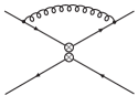
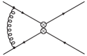
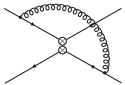
Figure 6: Feynman diagrams contributing at one loop to the four-fermion operator matrix elements in the effective theory.

Consistency in the matching procedure requires the matrix elements in the effective theory to be computed between the same set of external states and with the same regularization procedure for IR divergences adopted in the full theory. Therefore, we have performed this calculation by choosing massless quarks with zero momentum as external states and implementing separately the three regularization setups: DRED-$d$, DRED-$\lambda$ and NDR-$\lambda$. Note, in particular, that the bare amplitudes vanish identically at one loop in the DRED-$d$ scheme, since all loop integrals in this case reduce to tadpole massless integrals which vanish in dimensional regularization.

Eq. (4.1) also indicates that the one loop results for the bare matrix elements must be projected onto the basis of the physical operators. This projection implies a definition of the evanescent operators. In the DRED regularization scheme the only evanescent operators entering the calculation are defined to be proportional to the tensor $\Delta g_{\mu\nu}$ of eq. (3.2). Besides the operators specified in eq. (3.4), we also find the appearance of the evanescent operators

$$E^{\rm DRED}_{4} = \Delta g_{\mu\nu}\;\bar{d}^{i}{\sigma}^{\mu\rho}_{L}b^{i}\,\bar{d}^{j}{\sigma}^{\nu}_{\rho\,L}b^{j}~{},$$

$$E^{\rm DRED}_{5} = \Delta g_{\mu\nu}\;\bar{d}^{i}{\sigma}^{\mu\rho}_{L}b^{j}\,\bar{d}^{j}{\sigma}^{\nu}_{\rho\,L}b^{i}~{}.$$ (4.2)

In the NDR scheme, instead, both Dirac and Fierz evanescent operators must be introduced. Dirac evanescent operators are defined from the orthogonality condition to the Dirac projectors (see eq. (3.9)),

$${\rm Tr}\left[E_{A}^{(i)}\,P_{A}^{(j)}\,E_{B}^{(i)}\,P_{B}^{(j)}\right]=0~{}.$$ (4.3)

The complete list is given in ref. [8]. As for the Fierz evanescent operators, they are defined without introducing in the four dimensional Fierz relations arbitrary terms of $\mathcal{O}(\varepsilon)$; for example, the $\gamma_{\mu L}\otimes\gamma^{\mu}_{L}$ Fierz evanescent operator reads

$$E_{1}^{\rm NDR}=\bar{d}^{i}\gamma_{\mu L}b^{j}\,\bar{d}^{j}\gamma^{\mu}_{L}b^{i}-\bar{d}^{i}\gamma_{\mu L}b^{i}\,\bar{d}^{j}\gamma^{\mu}_{L}b^{j}$$ (4.4)

and similarly for the other gamma structures.

According to eq. (4.1), the second ingredient in the determination of the matrix $r$ is the one-loop calculation of the renormalization matrix $Z$. This requires again the evaluation of the Feynman diagrams shown in fig. 6. In this case however, in order to identify the UV divergences within dimensional regularization, one can either regularize the IR divergences with a fictitious gluon mass or consider a set of IR finite external states, for instance off-shell quarks with fixed momentum $p$.

In both the $\overline{\mbox{MS}}$-DRED and -NDR regularization schemes the renormalization matrix of the physical operators is determined by applying the modified minimal subtraction prescription. Evanescent operators, instead, must satisfy a different renormalization condition. For IR finite configurations of external states, this condition reads

$$\langle E_{i}(\mu)\rangle=0\quad\textrm{ in the limit}\;d\rightarrow 4~{},$$ (4.5)

and holds at any value of the renormalization scale $\mu$ [20]. It guarantees that the evanescent operators do not play any role when going back to four dimensions and can be eventually removed from the operator basis of the effective Hamiltonian.

The final result for the matrix $r$ defined in eq. (4.1) depends on several choices done in the calculation: the external states, the IR regulator (when IR divergences are present) and the renormalization scheme of the local operators. Thus we end up with three different matrices, $r^{{\rm DRED}-d}$, $r^{{\rm DRED}-\lambda}$ and $r^{{\rm NDR}-\lambda}$. Here we only present the results for the differences $\Delta r$ between these matrices because, at variance with the $r$’s, they are independent of the specific choice of both the external states and the IR regulator. As can be seen from eq. (4.1), the matrices $\Delta r$ provide the relation between operators renormalized in different schemes. In the case of the $\overline{\mbox{MS}}$-NDR and DRED schemes, for instance, this relation reads

$$\langle{\cal O}_{i}\rangle^{\rm\overline{\mbox{\scriptsize MS}}-NDR}=\left(1+\frac{\alpha_{s}}{4\pi}\Delta r^{\rm NDR/DRED}\right)_{ij}\langle{\cal O}_{j}\rangle^{\rm\overline{\mbox{\scriptsize MS}}-DRED}~{},$$ (4.6)

where $\Delta r^{\rm NDR/DRED}\equiv r^{\rm NDR}-r^{\rm DRED}$. For this matrix we obtain the result

$$\Delta r^{\rm NDR/DRED}=\left(\begin{array}[]{ccccc}-3&0&0&0&0\\ 0&-13/3&-1/3&0&0\\ 0&-29/6&7/6&0&0\\ 0&0&0&-5/3&-3\\ 0&0&0&-7/2&-1/6\\ \end{array}\right)~{},$$ (4.7)

in the basis ${\cal O}_{1},\ldots,{\cal O}_{5}$ of eq. (2.2). Since chirality is conserved by QCD interactions in the limit of massless quarks, the corresponding matrix for the operators $\tilde{{\cal O}}_{1,2,3}$ is equal to the $3\times 3$ submatrix for ${\cal O}_{1,2,3}$ in eq. (4.7) and the two sets of operators do not mix.

In addition, we provide the matrix $\Delta r$ relating the $\overline{\mbox{MS}}$-DRED with the so called RI-MOM scheme in the Landau gauge [21]. This is useful because this scheme is frequently used in lattice QCD calculations of the hadronic matrix elements. This matrix reads:

$$\Delta r^{\rm DRED/RI}=\left(\begin{array}[]{ccc}-\frac{5}{3}+8\,\ln 2&0&0\\[5.69046pt] 0&A_{2\times 2}&0\\[5.69046pt] 0&0&B_{2\times 2}\end{array}\right)~{},$$ (4.8)

with

$$A_{2\times 2}=\left(\begin{array}[]{cc}\frac{67}{9}+\frac{44}{9}\,\ln 2&-\frac{1}{9}+\frac{28}{9}\,\ln 2\\[5.69046pt] -\frac{28}{9}+\frac{28}{9}\,\ln 2&-\frac{68}{9}+\frac{44}{9}\,\ln 2\end{array}\right)$$ (4.9)

and

$$B_{2\times 2}=\left(\begin{array}[]{cc}13-\frac{2}{3}\,\ln 2&1+2\,\ln 2\\[5.69046pt] \frac{11}{2}+2\,\ln 2&-\frac{1}{2}-\frac{2}{3}\,\ln 2\end{array}\right)~{}.$$ (4.10)

The results in eqs. (4.7) and (4.8) can be also combined to obtain the matrix relating the $\overline{\mbox{MS}}$-NDR with the RI-MOM scheme: $\Delta r^{\rm NDR/RI}=\Delta r^{\rm NDR/DRED}+\Delta r^{\rm DRED/RI}$.

5 Results and checks of the calculation

In the previous sections we have described the calculation of the two ingredients needed to obtain the Wilson coefficients at the NLO: the LO and NLO amplitudes in the full theory, $F^{(0)}$ and $F^{(1)}$, and the matrix $r$ in the effective theory. The NLO Wilson coefficients are finally determined using eq. (2.5). They bear a dependence on both the renormalization scheme and scale. These dependences only arise at the NLO and allow one to perform useful checks of the calculation. The relations among the results for the coefficients as obtained in the three regularization setups, DRED-$\lambda$, NDR-$\lambda$ and DRED-$d$, will be discussed in the following subsection. The scale dependence of the Wilson coefficients must satisfy the renormalization group equation, and this constraint will be addressed in subsection 5.2.

5.1 Regularization and renormalization scheme dependence

The results for the coefficients obtained in the DRED-$\lambda$ setup must be equal to those obtained in DRED-$d$, since the Wilson coefficients cannot depend on the IR regulator. Indeed, upon explicit comparison, they are found to be in agreement. We emphasize that this is a non-trivial check of the calculation. Indeed, whereas the computation in the DRED-$\lambda$ scheme presents basically no subtlety, the one in the DRED-$d$ regularization entails the inclusion in the full theory of the LO contributions up to $O(\varepsilon)$ and of the evanescent operators. All these contributions should sum up to reconstruct the results obtained by using the gluon mass as IR regulator.

The results for the Wilson coefficients obtained in the $\overline{\mbox{MS}}$-DRED and NDR renormalization schemes differ because the coefficients are scheme dependent quantities. They can be compared using the scheme independence of the effective Hamiltonian:

$$\langle\overline{b},d|\mathcal{H}_{\rm eff}|b,\overline{d}\rangle=\sum_{i}C_{i}^{\rm DRED}\langle\overline{b},d|Q_{i}|b,\overline{d}\rangle^{\rm DRED}=C_{i}^{\rm NDR}\langle\overline{b},d|Q_{i}|b,\overline{d}\rangle^{\rm NDR}~{}.$$ (5.1)

The relation between renormalized operators in the two schemes has been written in eq. (4.6) in term of the matrix $\Delta r$. From eq. (5.1), it then follows that the same matrix also relates the coefficients in different schemes, e.g.

$$C_{i}^{\rm NDR}(M_{s},M_{\tilde{g}},\alpha_{s})=\sum_{j}\left(1-\frac{\alpha_{s}}{4\pi}\Delta r^{\rm NDR/DRED}\right)_{ji}C_{j}^{\rm DRED}(M_{s},M_{\tilde{g}},\alpha_{s})~{},$$ (5.2)

where $\Delta r^{\rm NDR/DRED}$ is given in eq. (4.7). Notice that in eq. (5.2) the transposed matrix $\Delta r^{T}$ enters. The coupling constant $\alpha_{s}$ and the SUSY masses $M_{s}$ and $M_{\tilde{g}}$ in the previous equation are also scheme dependent quantities. This dependence starts at $O(\alpha_{s})$ and must be taken into account in the matching at the NLO. In order to verify eq. (5.2), therefore, one needs to express all the couplings in the same scheme. The required relations are [22]:

$$\hat{\alpha}_{s}^{\rm NDR}=\alpha_{s}^{\rm DRED}\left(1+\frac{\alpha_{s}}{4\pi}(N_{c}-C_{F})\right)$$

$$M^{\rm NDR}_{\tilde{g}}=M^{\rm DRED}_{\tilde{g}}\left(1+\frac{\alpha_{s}}{4\pi}N_{c}\right)$$ (5.3)

$$M^{\rm NDR}_{s}=M^{\rm DRED}_{s}\left(1+\mathcal{O}(\alpha_{s}^{2})\right)~{},$$

where $N_{c}=3$ and $C_{F}=4/3$ are the SU(3$)_{c}$ color factors. The strong coupling constant $\hat{\alpha}_{s}$ in eq. (5.3) indicates the coupling of the quark-squark-gluino vertex. A different relation is found for the quark-quark-gluon coupling, which differs from $\hat{\alpha}_{s}$ in the NDR scheme because this regularization breaks supersymmetry [22] (see eq. (A.3)). In the present calculation, since the shifts expressed by eq. (5.3) are ${\cal O}(\alpha_{s})$, they have to be implemented only in the LO amplitude, where only the coupling $\hat{\alpha}_{s}$ appears. We find that our results for the Wilson coefficients as obtained in the DRED and NDR schemes consistently satisfy eq. (5.2), with the matrix $\Delta r^{\rm NDR/DRED}$ given in eq. (4.7).

5.2 Renormalization scale dependence

Beyond LO, the Wilson coefficients acquire an explicit dependence on the renormalization scale $\mu$. This dependence is controlled by the renormalization group equation, which provides therefore an additional check of the calculation.

The renormalization group equation for the Wilson coefficients of the MSSM [23, 24] can be written as

$$\left[\frac{\partial}{\partial\ln\mu^{2}}+\frac{d\alpha_{s}}{d\ln\mu^{2}}\frac{\partial}{\partial\alpha_{s}}+\frac{dM_{\tilde{g}}^{2}}{d\ln\mu^{2}}\frac{\partial}{\partial M_{\tilde{g}}^{2}}+\frac{dM_{s}^{2}}{d\ln\mu^{2}}\frac{\partial}{\partial M_{s}^{2}}+\sum_{X}\frac{d\Delta_{X}}{d\ln\mu^{2}}\frac{\partial}{\partial\Delta_{X}}\right.$$

$$\qquad\left.-\frac{1}{2}\gamma^{T}\right]\vec{C}(\mu)=0~{},$$ (5.4)

and takes into account the scale dependence of all the quantities entering the coefficients, namely the strong coupling constant $\alpha_{s}$, the squark and gluino masses $M_{s}$ and $M_{\tilde{g}}$ and the dimensionful mass insertions $\Delta_{X}$, with $X=LL,\,RR,\,LR\,,RL$.

The matrix $\gamma$ in eq. (5.4) is the anomalous dimension matrix of the four-fermion operators (2.2) in the effective theory (i.e. QCD). It can be expanded as

$$\gamma(\alpha_{s})=Z^{-1}\frac{dZ}{d\ln\mu}=\frac{\alpha_{s}}{4\pi}\,\gamma_{0}+\mathcal{O}(\alpha_{s}^{2})$$ (5.5)

where, for the LO anomalous dimension $\gamma_{0}$, we obtain the expression

$$\gamma_{0}=\left(\begin{array}[]{ccccc}4&0&0&0&0\\ 0&-28/3&4/3&0&0\\ 0&16/3&32/3&0&0\\ 0&0&0&-16&0\\ 0&0&0&-6&2\\ \end{array}\right)~{},$$ (5.6)

in agreement with eqs. (11)-(13) of ref. [25].

The renormalization group equation for the strong coupling constant in the MSSM reads

$$\beta^{\rm MSSM}(\alpha_{s})=\frac{d\alpha_{s}}{d\ln\mu^{2}}=-\frac{\alpha_{s}^{2}}{4\pi}\,\beta_{0}^{\rm MSSM}+\mathcal{O}(\alpha_{s}^{3})~{},$$ (5.7)

with $\beta_{0}^{\rm MSSM}=3N_{c}-N_{f}$.

The scale dependence of the squark and gluino masses, $M_{s}$ and $M_{\tilde{g}}$, is described instead by the equations

$$\gamma_{M_{i}}(\alpha_{s})=\frac{1}{M_{i}^{2}}\frac{dM_{i}^{2}}{d\ln\mu^{2}}=-\frac{\alpha_{s}}{4\pi}\,\gamma^{(0)}_{M_{i}}+O(\alpha_{s}^{2})\qquad,\qquad i={s,\tilde{g}}~{},$$ (5.8)

where $\gamma^{(0)}_{M_{s}}=4C_{F}M_{\tilde{g}}^{2}/M_{s}^{2}$ and $\gamma^{(0)}_{M_{\tilde{g}}}=2\beta_{0}^{\rm MSSM}=2(3N_{c}-N_{f})$.

Finally, the running of the dimensionful mass insertions $\Delta_{X}$ is expressed by

$$\frac{d\Delta_{LL(RR)}}{d\ln\mu^{2}}=0+O(\alpha_{s}^{2})~{},$$

$$\frac{d\Delta_{LR(RL)}}{d\ln\mu^{2}}=-\frac{\alpha_{s}}{4\pi}\,\gamma^{(0)}_{\Delta}\Delta_{LR(RL)}+O(\alpha_{s}^{2})$$ (5.9)

with $\gamma^{(0)}_{\Delta}=2C_{F}$.

By using the results given in eqs. (5.7)-(5.9), we have then verified that our expressions for the Wilson coefficients exhibit at the NLO the correct renormalization scale dependence predicted by eq. (5.4).

5.3 Discussion of the results

We conclude this section by presenting and discussing the final results obtained for the Wilson coefficients at the NLO. The complete expressions of these coefficients, in the $\overline{\mbox{MS}}$-DRED renormalization scheme, are collected in appendix A.

In order to illustrate the typical size of the computed NLO corrections, we show in fig. 7 the values of the NLO contributions to the Wilson coefficients normalized to their expected size, namely the corresponding LO coefficients multiplied by $\alpha_{s}(M_{s})/\pi$. For the purpose of illustration, in this comparison we set the scale $\mu=M_{s}$ and put $M_{\tilde{g}}=M_{s}$.

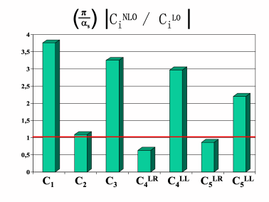
Figure 7: Comparison between the LO and NLO contributions to the $\overline{\mbox{MS}}$-DRED Wilson coefficients at the scale $\mu=M_{s}$ and at the reference value $M_{\tilde{g}}=M_{s}$. For the coefficients $C_{4}$ and $C_{5}$ the contributions proportional to $\delta_{LL}\delta_{RR}$ and $\delta_{LR}\delta_{RL}$ are shown separately.

As can be seen from the plot, in several cases the NLO coefficients turn out to be larger than what naively expected. Of course, this conclusion applies to the $\overline{\mbox{MS}}$-DRED coefficients and could change in a different renormalization scheme.

The Wilson coefficients depend on the matching scale $\mu$ which can be chosen around a typical SUSY scale, e.g. the average squark mass $M_{s}$. An important achievement of the NLO calculation is a significant reduction of this dependence with respect to the LO approximation. This is illustrated in fig. 8 where we show the LO and NLO predictions for the $B_{d}$-mesons mass difference $\Delta m_{d}$ as a function of the high-energy scale $\mu$ chosen for the matching. These predictions are obtained by adding the SUSY contributions to the reference SM value, $\Delta m_{d}^{\rm SM}=0.496$ ps^-1. The hadronic matrix elements are evaluated by using the lattice QCD results of ref. [26] for the B-parameters and $f_{B_{d}}=189$ MeV. We set $M_{s}=M_{\tilde{g}}=350$ GeV and consider two cases for mass insertion coefficients, $\delta_{LL}=\delta_{RR}=0.12\exp[-i\,23^{\rm o}]$ (upper plot in fig. 8) and $\delta_{LR}=\delta_{RL}=0.026\exp[-i\,23^{\rm o}]$ (lower plot in fig. 8), chosen to give a SUSY contribution compatible with the present measurement taking into account the SM uncertainty. Clearly, the reduction of the scale dependence found at the NLO quantitatively depends on the specific values chosen for the mass insertion parameters.

Figure 8: LO and NLO predictions for the $B_{d}$-mesons mass difference $\Delta m_{d}$ obtained by adding the SUSY contributions proportional to $\delta_{LL},\delta_{RR}$ (top) and $\delta_{LR},\delta_{RL}$ (bottom) to the SM prediction. See text for the reference values of the input parameters. The results are plotted as functions of the matching scale $\mu$.

From fig. 8 we see that the SUSY prediction for $\Delta m_{d}$ varies, at the LO, by approximately $\pm 16\%$ ($\pm 8\%$) in the LL/RR (LR/RL) case, when the scale $\mu$ is varied in the typical range between $M_{s}/2$ and $2M_{s}$. With the NLO calculation, the dependence on the matching scale is reduced by a factor two or more, i.e. at the level of $\pm 5\%$ ($\pm 2\%$) percent.

We conclude this section by observing that phenomenological applications require the knowledge of the hadronic matrix elements. These are usually computed on the lattice where, in order to perform a fully non-perturbative renormalization, the RI-MOM renormalization scheme [21] is needed. This is the scheme adopted for instance in refs. [27, 28] and [26], where lattice results for the complete basis of four-fermion operator matrix elements relevant for $K-\overline{K}$ and $B_{d,s}-\overline{B}_{d,s}$ systems have been presented. In these cases, the results for the Wilson coefficients given in appendix A in the $\overline{\mbox{MS}}$-DRED scheme must be converted to the RI-MOM scheme. This can be easily done using the relation analogous to eq. (5.2), namely

$$C_{i}^{\rm RI}=\sum_{j}\left(1+\frac{\alpha_{s}}{4\pi}\Delta r^{\rm DRED/RI}\right)^{\mathrm{T}}_{ij}C_{j}^{\rm\overline{\mbox{\scriptsize MS}}-DRED}~{}.$$ (5.10)

The matrix $(\Delta r^{\rm DRED/RI})^{\mathrm{T}}$ which performs the matching between the two schemes can be obtained by transposing the matrix in eq. (4.8).

6 Conclusions

In this work we have computed the NLO strong interaction corrections to the Wilson coefficients relevant for $\Delta F=2$ transitions in the MSSM with the mass insertion approximation. The complete expressions for the coefficients are given in appendix A in the $\overline{\mbox{MS}}$-DRED scheme. We also give in eqs. (5.2) and (5.10) the formulae required to translate the Wilson coefficients at the NLO from the DRED to the NDR and the RI-MOM renormalization schemes, which might be useful for phenomenological applications.

Theoretically, the NLO calculation of the Wilson coefficients is required to cancel the corresponding renormalization scale and scheme dependence of the renormalized operators. Once combined with the NLO anomalous dimension of the four-fermion operators given in ref. [7], our results allow to perform a complete NLO analysis of $\Delta F=2$ transitions in the MSSM. The phenomenological analysis will be presented in a forthcoming publication. In this study we have shown that, by considering as a reference example the theoretical prediction of the $B_{d}$-meson mass difference $\Delta m_{d}$, the uncertainty due to the choice of the the high-energy matching scale is largely reduced going from the LO to the NLO, typically from about 10-15% to few percent.

Appendix A Results for the Wilson coefficients

In this appendix we collect the complete NLO expressions of the Wilson coefficients entering the effective Hamiltonian which describes $\Delta F=2$ transitions mediated by strong interactions in the MSSM.

We consider the complete basis of four fermion operators given in eq. (2.2). The coefficients for the operators $\tilde{Q}_{1,2,3}$ are obtained from those of the operators $Q_{1,2,3}$ by simply exchanging $L\leftrightarrow R$ in the mass insertion parameters. For this reason, we will not present in the following their explicit expressions.

The Wilson coefficients are written as

$$C_{i}(\mu)=C_{i}^{(0)}(\mu)+C_{i}^{(1)}(\mu)\,,$$ (A.1)

where $\mu$ is the scale used in the matching procedure. To simplify the notation, in the following, we will not write explicitly the $\mu$ dependence of masses and couplings.

The LO calculation of the Wilson coefficients has been performed in ref. [3] and we agree with their results. These coefficients read

$$C_{1}^{(0)}(\mu)=\frac{\alpha_{s}^{2}}{(1-x)^{5}\,M_{s}^{2}}\Big{[}\frac{11}{108}+\frac{133\,x}{108}-\frac{13\,{x^{2}}}{12}-\frac{29\,{x^{3}}}{108}+\frac{{x^{4}}}{54}+\big{(}\frac{13\,x}{18}+\frac{17\,{x^{2}}}{18}\big{)}\,\log x\Big{]}\,\delta_{{LL}}^{2}$$

$$C_{2}^{(0)}(\mu)=\frac{\alpha_{s}^{2}}{(1-x)^{5}\,M_{s}^{2}}\Big{[}\frac{289\,x}{108}-\frac{17\,{x^{2}}}{12}-\frac{17\,{x^{3}}}{12}+\frac{17\,{x^{4}}}{108}+\big{(}\frac{17\,x}{18}+\frac{17\,{x^{2}}}{6}\big{)}\,\log x\Big{]}\,\delta_{{RL}}^{2}$$

$$C_{3}^{(0)}(\mu)=\frac{\alpha_{s}^{2}}{(1-x)^{5}\,M_{s}^{2}}\Big{[}-\frac{17\,x}{36}+\frac{{x^{2}}}{4}+\frac{{x^{3}}}{4}-\frac{{x^{4}}}{36}-\big{(}\frac{x}{6}+\frac{{x^{2}}}{2}\big{)}\,\log x\Big{]}\,\delta_{{RL}}^{2}$$

$$C_{4}^{(0)}(\mu)=\frac{\alpha_{s}^{2}}{{{(1-x)}^{5}}\,M_{s}^{2}}\Big{[}\Big{(}-\frac{11}{54}-\frac{11\,x}{6}+\frac{11\,{x^{2}}}{6}+\frac{11\,{x^{3}}}{54}-\frac{11\,x}{9}\big{(}1+x\big{)}\,\log x\Big{)}\,{{\delta}_{{LR}}}\,{{\delta}_{{RL}}}+$$

$$\qquad\Big{(}-\frac{1}{9}+\frac{101\,x}{18}-\frac{5\,{x^{2}}}{2}-\frac{61\,{x^{3}}}{18}+\frac{7\,{x^{4}}}{18}+\Big{(}\frac{5\,x}{3}+\frac{19\,{x^{2}}}{3}\Big{)}\,\log x\Big{)}\,{{\delta}_{{LL}}}\,{{\delta}_{{RR}}}\Big{]}$$

$$C_{5}^{(0)}(\mu)=\frac{\alpha_{s}^{2}}{(1-x)^{5}\,M_{s}^{2}}\Big{[}\Big{(}-\frac{5}{18}-\frac{5\,x}{2}+\frac{5\,{x^{2}}}{2}+\frac{5\,{x^{3}}}{18}-\frac{5\,x}{3}\big{(}1+x\big{)}\,\log x\Big{)}\,{{\delta}_{{LR}}}\,{{\delta}_{{RL}}}+$$

$$\qquad\Big{(}\frac{5}{27}+\frac{107\,x}{54}-\frac{11\,{x^{2}}}{6}-\frac{19\,{x^{3}}}{54}+\frac{{x^{4}}}{54}+\Big{(}\frac{11\,x}{9}+\frac{13\,{x^{2}}}{9}\Big{)}\,\log x\Big{)}\,{{\delta}_{{LL}}}\,{{\delta}_{{RR}}}\Big{]}$$ (A.2)

where $x=M_{\tilde{g}}^{2}/M_{s}^{2}$ with $M_{\tilde{g}}$ the gluino mass and $M_{s}$ the average squark mass. The dimensionless mass insertion parameters are understood to be $\delta_{12}^{d}$, $\delta_{13}^{d}$, $\delta_{23}^{d}$ and $\delta_{12}^{u}$ for the cases of $K$, $B_{d}$, $B_{s}$ and $D$ mixings respectively.

At the NLO, the Wilson coefficients are scheme dependent quantities. Here we present the results for the operators renormalized in the $\overline{\mbox{MS}}$-DRED scheme, and we adopt the same scheme also for the strong coupling constant $\alpha_{s}(\mu)$ and for the squark and gluino masses. Eq. (5.10) can be then used to convert the coefficients to the RI-MOM scheme, frequently adopted in lattice QCD calculations of the corresponding hadronic matrix elements. As for the strong coupling constant and the squark and gluino masses, they can be converted to their counterparts in the $\overline{\mbox{MS}}$-NDR scheme by using [29, 22]

$$\alpha_{s}^{\rm NDR}=\alpha_{s}^{\rm DRED}\left(1-\frac{\alpha_{s}}{4\pi}\frac{N_{c}}{3}\right)$$

$$M^{\rm NDR}_{\tilde{g}}=M^{\rm DRED}_{\tilde{g}}\left(1+\frac{\alpha_{s}}{4\pi}N_{c}\right)$$ (A.3)

$$M^{\rm NDR}_{s}=M^{\rm DRED}_{s}\left(1+\mathcal{O}(\alpha_{s}^{2})\right)~{}.$$

We now present the NLO expressions for the Wilson coefficients. In the following, the symbol $\rm{Li}_{2}(x)$ denotes the dilogarithm function defined as

$$\rm{Li}_{2}(x)=-\int_{0}^{x}\frac{dt}{t}\ln(1-t)~{}$$ (A.4)

and all couplings and masses are understood to be renormalized at the same scale $\mu$. The coefficients read

$$C_{1}^{(1)}(\mu)=\frac{\alpha_{s}^{3}}{\pi M_{s}^{2}}\ \frac{1}{(1-x)^{7}}\cdot$$

$$\qquad{\delta_{LL}}^{2}\,\Big{[}\frac{4171}{864}+\frac{50197\,x}{2592}-\frac{9911\,x^{2}}{144}+\frac{25039\,x^{3}}{432}-\frac{27371\,x^{4}}{2592}-\frac{317\,x^{5}}{96}+\frac{7\,x^{6}}{12}-\frac{4\,x^{7}}{81}+$$

$$\qquad\Big{(}\frac{55\,x}{9}+\frac{17005\,x^{2}}{1296}-\frac{3607\,x^{3}}{144}+\frac{4319\,x^{4}}{1296}+\frac{3875\,x^{5}}{1296}-\frac{5\,x^{6}}{9}+\frac{4\,x^{7}}{81}\ \Big{)}\,\log x+$$

$$\qquad\Big{(}-\frac{247\,x}{72}-\frac{1079\,x^{2}}{72}+\frac{3721\,x^{3}}{216}+\frac{497\,x^{4}}{216}\Big{)}\,\log^{2}x+$$

$$\qquad\Big{(}-\frac{229}{108}+\frac{691\,x}{108}+\frac{67\,x^{2}}{36}-\frac{1559\,x^{3}}{108}+\frac{224\,x^{4}}{27}\Big{)}\,{\rm Li}_{2}(1-x)+$$

$$\qquad\log\Big{(}\frac{M_{s}^{2}}{\mu^{2}}\Big{)}\,\Big{(}-\frac{11}{54}-\frac{577\,x}{108}+\frac{1094\,x^{2}}{81}-\frac{2389\,x^{3}}{324}-\frac{1255\,x^{4}}{324}+\frac{310\,x^{5}}{81}-\frac{191\,x^{6}}{324}+\frac{4\,x^{7}}{81}+$$

$$\qquad\Big{(}-\frac{91\,x}{36}-\frac{133\,x^{2}}{108}+\frac{935\,x^{3}}{108}-\frac{529\,x^{4}}{108}\Big{)}\,\log x\Big{)}\Big{]}$$ (A.5)

$$C_{2}^{(1)}(\mu)=\frac{\alpha_{s}^{3}}{\pi M_{s}^{2}}\ \frac{1}{(1-x)^{7}}\cdot$$

$$\qquad{\delta_{RL}}^{2}\,\Big{[}\frac{311827\,x}{3888}-\frac{783947\,x^{2}}{3888}+\frac{308057\,x^{3}}{1944}-\frac{58433\,x^{4}}{1944}-\frac{39589\,x^{5}}{3888}+\frac{14093\,x^{6}}{3888}-\frac{34\,x^{7}}{81}+$$

$$\qquad\Big{(}\frac{107\,x}{9}+\frac{2285\,x^{2}}{108}-\frac{5839\,x^{3}}{162}-\frac{109\,x^{4}}{81}+\frac{41\,x^{5}}{6}-\frac{943\,x^{6}}{324}+\frac{34\,x^{7}}{81}\Big{)}\,\log x+$$

$$\qquad\Big{(}-\frac{199\,x}{216}-\frac{7535\,x^{2}}{216}+\frac{5869\,x^{3}}{216}+\frac{803\,x^{4}}{72}\Big{)}\,\log^{2}x+$$

$$\qquad\Big{(}-\frac{191\,x}{18}+\frac{2011\,x^{2}}{54}-\frac{2303\,x^{3}}{54}+\frac{865\,x^{4}}{54}\Big{)}\,{\rm Li}_{2}(1-x)+$$

$$\qquad\log\Big{(}\frac{M_{s}^{2}}{\mu^{2}}\Big{)}\,\Big{(}-\frac{6205\,x}{648}+\frac{10891\,x^{2}}{648}+\frac{2077\,x^{3}}{324}-\frac{9035\,x^{4}}{324}+\frac{11411\,x^{5}}{648}-\frac{2453\,x^{6}}{648}+\frac{34\,x^{7}}{81}+$$

$$\qquad\Big{(}-\frac{311\,x}{108}-\frac{991\,x^{2}}{108}+\frac{2575\,x^{3}}{108}-\frac{1273\,x^{4}}{108}\Big{)}\,\log x\ \Big{)}\Big{]}$$ (A.6)

$$C_{3}^{(1)}(\mu)=\frac{\alpha_{s}^{3}}{\pi M_{s}^{2}}\ \frac{1}{(1-x)^{7}}\cdot$$

$$\qquad{\delta_{RL}}^{2}\,\Big{[}-\frac{43993\,x}{3888}+\frac{103649\,x^{2}}{3888}-\frac{35339\,x^{3}}{1944}+\frac{2147\,x^{4}}{1944}+\frac{9103\,x^{5}}{3888}-\frac{2663\,x^{6}}{3888}+\frac{2\,x^{7}}{27}+$$

$$\qquad\Big{(}\frac{43\,x}{27}-\frac{3677\,x^{2}}{324}+\frac{1537\,x^{3}}{162}+\frac{59\,x^{4}}{27}-\frac{401\,x^{5}}{162}+\frac{205\,x^{6}}{324}-\frac{2\,x^{7}}{27}\Big{)}\,\log x+$$

$$\qquad\Big{(}\frac{277\,x}{216}+\frac{55\,x^{2}}{8}-\frac{175\,x^{3}}{24}-\frac{283\,x^{4}}{216}\Big{)}\,\log^{2}x+$$

$$\qquad\Big{(}\frac{71\,x}{54}-\frac{385\,x^{2}}{54}+\frac{557\,x^{3}}{54}-\frac{9\,x^{4}}{2}\Big{)}\,{\rm Li}_{2}(1-x)+$$

$$\qquad\log\Big{(}\frac{M_{s}^{2}}{\mu^{2}}\Big{)}\,\Big{(}\frac{1607\,x}{648}-\frac{3217\,x^{2}}{648}+\frac{25\,x^{3}}{324}+\frac{1745\,x^{4}}{324}-\frac{2345\,x^{5}}{648}+\frac{463\,x^{6}}{648}-\frac{2\,x^{7}}{27}+$$

$$\qquad\Big{(}\frac{85\,x}{108}+\frac{205\,x^{2}}{108}-\frac{605\,x^{3}}{108}+\frac{35\,x^{4}}{12}\Big{)}\,\log x\ \Big{)}\Big{]}$$ (A.7)

$$C_{4}^{(1)}(\mu)=\frac{\alpha_{s}^{3}}{\pi M_{s}^{2}}\ \frac{1}{(1-x)^{7}}\cdot\Big{\{}$$

$$\qquad\delta_{LL}\,\delta_{RR}\,\Big{[}-\frac{203}{36}+\frac{39341\,x}{216}-\frac{91895\,x^{2}}{216}+\frac{33707\,x^{3}}{108}-\frac{733\,x^{4}}{18}-\frac{6691\,x^{5}}{216}+\frac{2069\,x^{6}}{216}-\frac{28\,x^{7}}{27}+$$

$$\qquad\Big{(}\frac{31\,x}{12}+\frac{8435\,x^{2}}{108}-\frac{7927\,x^{3}}{108}-\frac{2065\,x^{4}}{108}+\frac{490\,x^{5}}{27}-\frac{397\,x^{6}}{54}+\frac{28\,x^{7}}{27}\ \Big{)}\,\log x+$$

$$\qquad\Big{(}-\frac{43\,x}{8}-\frac{1873\,x^{2}}{24}+\frac{4687\,x^{3}}{72}+\frac{1703\,x^{4}}{72}\Big{)}\,\log^{2}x\ +$$

$$\qquad\Big{(}\frac{49}{18}-\frac{721\,x}{18}+\frac{599\,x^{2}}{6}-\frac{1627\,x^{3}}{18}+\frac{251\,x^{4}}{9}\ \Big{)}\,{\rm Li}_{2}(1-x)+$$

$$\qquad\log\Big{(}\frac{M_{s}^{2}}{\mu^{2}}\Big{)}\,\Big{(}\frac{1}{12}-\frac{461\,x}{72}-\frac{413\,x^{2}}{216}+\frac{4529\,x^{3}}{108}-\frac{1600\,x^{4}}{27}+\frac{7109\,x^{5}}{216}-\frac{1813\,x^{6}}{216}+\frac{28\,x^{7}}{27}+$$

$$\qquad\Big{(}-\frac{3\,x}{4}-\frac{607\,x^{2}}{36}+\frac{1055\,x^{3}}{36}-\frac{421\,x^{4}}{36}\Big{)}\,\log x\ \Big{)}\Big{]}+$$

$$\qquad\delta_{LR}\,\delta_{RL}\,\Big{[}-\frac{15031}{1296}-\frac{6875\,x}{1296}+\frac{33709\,x^{2}}{648}-\frac{20747\,x^{3}}{648}-\frac{16963\,x^{4}}{1296}+\frac{13297\,x^{5}}{1296}-\frac{22\,x^{6}}{81}+$$

$$\qquad\Big{(}\frac{163\,x}{36}-\frac{26977\,x^{2}}{648}+\frac{25831\,x^{3}}{648}+\frac{359\,x^{4}}{216}-\frac{3041\,x^{5}}{648}+\frac{22\,x^{6}}{81}\Big{)}\,\log x+$$

$$\qquad\Big{(}\frac{103\,x}{8}+\frac{703\,x^{2}}{72}-\frac{4969\,x^{3}}{216}-\frac{91\,x^{4}}{72}\Big{)}\,\log^{2}x+$$

$$\qquad\Big{(}\frac{385}{108}-\frac{217\,x}{54}-\frac{13\,x^{2}}{3}+\frac{349\,x^{3}}{54}-\frac{181\,x^{4}}{108}\ \Big{)}\,{\rm Li}_{2}(1-x)+$$

$$\qquad\log\Big{(}\frac{M_{s}^{2}}{\mu^{2}}\Big{)}\,\Big{(}-\frac{25}{648}+\frac{3257\,x}{648}-\frac{3481\,x^{2}}{324}+\frac{1369\,x^{3}}{324}+\frac{2683\,x^{4}}{648}-\frac{1867\,x^{5}}{648}+\frac{22\,x^{6}}{81}+$$

$$\qquad\Big{(}\frac{173\,x}{108}+\frac{311\,x^{2}}{108}-\frac{307\,x^{3}}{36}+\frac{437\,x^{4}}{108}\Big{)}\,\log x\ \Big{)}\Big{]}\Big{\}}$$ (A.8)

$$C_{5}^{(1)}(\mu)=\frac{\alpha_{s}^{3}}{\pi M_{s}^{2}}\ \frac{1}{(1-x)^{7}}\cdot\Big{\{}$$

$$\qquad\delta_{LL}\,\delta_{RR}\,\Big{[}\frac{305}{36}+\frac{6521\,x}{216}-\frac{72913\,x^{2}}{648}+\frac{31549\,x^{3}}{324}-\frac{3193\,x^{4}}{162}-\frac{2885\,x^{5}}{648}+\frac{451\,x^{6}}{648}-\frac{4\,x^{7}}{81}+$$

$$\qquad\Big{(}\frac{361\,x}{36}+\frac{1775\,x^{2}}{108}-\frac{10505\,x^{3}}{324}+\frac{929\,x^{4}}{324}+\frac{100\,x^{5}}{27}-\frac{107\,x^{6}}{162}+\frac{4\,x^{7}}{81}\ \Big{)}\,\log x+$$

$$\qquad\Big{(}-\frac{407\,x}{72}-\frac{653\,x^{2}}{24}+\frac{6361\,x^{3}}{216}+\frac{1121\,x^{4}}{216}\Big{)}\,\log^{2}x+$$

$$\qquad\Big{(}-\frac{209}{54}+\frac{641\,x}{54}-\frac{7\,x^{2}}{18}-\frac{1045\,x^{3}}{54}+\frac{317\,x^{4}}{27}\ \Big{)}\,{\rm Li}_{2}(1-x)+$$

$$\qquad\log\Big{(}\frac{M_{s}^{2}}{\mu^{2}}\Big{)}\,\Big{(}-\frac{35}{108}-\frac{1787\,x}{216}+\frac{13765\,x^{2}}{648}-\frac{4057\,x^{3}}{324}-\frac{370\,x^{4}}{81}+\frac{3299\,x^{5}}{648}-\frac{451\,x^{6}}{648}+\frac{4\,x^{7}}{81}+$$

$$\qquad\Big{(}-\frac{143\,x}{36}-\frac{169\,x^{2}}{108}+\frac{1385\,x^{3}}{108}-\frac{787\,x^{4}}{108}\Big{)}\,\log x\ \Big{)}\Big{]}+$$

$$\qquad\delta_{LR}\,\delta_{RL}\,\Big{[}-\frac{5425}{432}-\frac{12125\,x}{432}+\frac{26875\,x^{2}}{216}-\frac{24125\,x^{3}}{216}+\frac{10715\,x^{4}}{432}+\frac{1495\,x^{5}}{432}-\frac{10\,x^{6}}{27}+$$

$$\qquad\Big{(}-\frac{155\,x}{12}-\frac{5095\,x^{2}}{216}+\frac{10465\,x^{3}}{216}-\frac{655\,x^{4}}{72}-\frac{695\,x^{5}}{216}+\frac{10\,x^{6}}{27}\Big{)}\,\log x+$$

$$\qquad\Big{(}\frac{75\,x}{8}+\frac{625\,x^{2}}{24}-\frac{2455\,x^{3}}{72}-\frac{85\,x^{4}}{24}\Big{)}\,\log^{2}x+$$

$$\qquad\Big{(}\frac{175}{36}-\frac{295\,x}{18}+5\,x^{2}+\frac{355\,x^{3}}{18}-\frac{475\,x^{4}}{36}\Big{)}\,{\rm Li}_{2}(1-x)+$$

$$\qquad\log\Big{(}\frac{M_{s}^{2}}{\mu^{2}}\Big{)}\,\Big{(}\frac{185}{216}+\frac{2855\,x}{216}-\frac{4135\,x^{2}}{108}+\frac{3175\,x^{3}}{108}-\frac{155\,x^{4}}{216}-\frac{1045\,x^{5}}{216}+\frac{10\,x^{6}}{27}+$$

$$\qquad\Big{(}\frac{275\,x}{36}-\frac{55\,x^{2}}{36}-\frac{205\,x^{3}}{12}+\frac{395\,x^{4}}{36}\Big{)}\,\log x\ \Big{)}\Big{]}\Big{\}}$$ (A.9)

References

- [1] L. J. Hall, V. A. Kostelecky, and S. Raby, New flavor violations in supergravity models, Nucl. Phys. B267 (1986) 415.
- [2] J. M. Gerard, W. Grimus, A. Raychaudhuri, and G. Zoupanos, Super Kobayashi-Maskawa CP violation, Phys. Lett. B140 (1984) 349.
- [3] F. Gabbiani, E. Gabrielli, A. Masiero, and L. Silvestrini, A complete analysis of FCNC and CP constraints in general SUSY extensions of the Standard Model, Nucl. Phys. B477 (1996) 321–352, [hep-ph/9604387].
- [4] F. Krauss and G. Soff, Next-to-leading order QCD corrections to B anti-B mixing and epsilon(k) within the MSSM, Nucl. Phys. B633 (2002) 237–249, [hep-ph/9807238].
- [5] J. Urban, F. Krauss, U. Jentschura, and G. Soff, Next-to-leading order QCD corrections for the B0 anti-B0 mixing with an extended Higgs sector, Nucl. Phys. B523 (1998) 40–58, [hep-ph/9710245].
- [6] T.-F. Feng, X.-Q. Li, W.-G. Ma, and F. Zhang, Complete analysis on the NLO SUSY-QCD corrections to B0- anti-B0 mixing, Phys. Rev. D63 (2001) 015013, [hep-ph/0008029].
- [7] M. Ciuchini et al., Next-to-leading order QCD corrections to effective Hamiltonians, Nucl. Phys. B523 (1998) 501–525, [hep-ph/9711402].
- [8] A. J. Buras, M. Misiak, and J. Urban, Two-loop QCD anomalous dimensions of flavour-changing four- quark operators within and beyond the Standard Model, Nucl. Phys. B586 (2000) 397–426, [hep-ph/0005183].
- [9] M. Ciuchini et al., Nlo calculation of the delta(f) = 2 hamiltonians in the mssm and phenomenological analysis of the b - anti-b mixing, PoS HEP2005 (2006) 221, [hep-ph/0512141].
- [10] H. E. Haber and G. L. Kane, The search for supersymmetry: Probing physics beyond the Standard Model, Phys. Rept. 117 (1985) 75.
- [11] A. Denner, H. Eck, O. Hahn, and J. Kublbeck, Feynman rules for fermion number violating interactions, Nucl. Phys. B387 (1992) 467–484.
- [12] A. J. Buras and P. H. Weisz, QCD nonleading corrections to weak decays in dimensional regularization and ’t Hooft-Veltman schemes, Nucl. Phys. B333 (1990) 66.
- [13] S. Wolfram, Mathematica – A system for doing mathematics by computer. Addison-Wesley Publishing Company Inc., 1988.
- [14] T. Hahn, Generating Feynman diagrams and amplitudes with FeynArts 3, Comput. Phys. Commun. 140 (2001) 418–431, [hep-ph/0012260]. and references therein. See also http://www.feynarts.de/.
- [15] K. G. Chetyrkin and F. V. Tkachov, Integration by parts: The algorithm to calculate beta functions in 4 loops, Nucl. Phys. B192 (1981) 159–204.
- [16] O. V. Tarasov, Connection between Feynman integrals having different values of the space-time dimension, Phys. Rev. D54 (1996) 6479–6490, [hep-th/9606018].
- [17] O. V. Tarasov, Generalized recurrence relations for two-loop propagator integrals with arbitrary masses, Nucl. Phys. B502 (1997) 455–482, [hep-ph/9703319].
- [18] R. Mertig and R. Scharf, TARCER: A Mathematica program for the reduction of two-loop propagator integrals, Comput. Phys. Commun. 111 (1998) 265–273, [hep-ph/9801383].
- [19] A. I. Davydychev and J. B. Tausk, Two loop selfenergy diagrams with different masses and the momentum expansion, Nucl. Phys. B397 (1993) 123–142.
- [20] M. J. Dugan and B. Grinstein, On the vanishing of evanescent operators, Phys. Lett. B256 (1991) 239–244.
- [21] G. Martinelli, C. Pittori, C. T. Sachrajda, M. Testa, and A. Vladikas, A general method for nonperturbative renormalization of lattice operators, Nucl. Phys. B445 (1995) 81–108, [hep-lat/9411010].
- [22] S. P. Martin and M. T. Vaughn, Regularization dependence of running couplings in softly broken supersymmetry, Phys. Lett. B318 (1993) 331–337, [hep-ph/9308222].
- [23] S. Bertolini, F. Borzumati, A. Masiero, and G. Ridolfi, Effects of supergravity induced electroweak breaking on rare B decays and mixings, Nucl. Phys. B353 (1991) 591–649.
- [24] R. Barbieri, L. J. Hall, and A. Strumia, Violations of lepton flavor and CP in supersymmetric unified theories, Nucl. Phys. B445 (1995) 219–251, [hep-ph/9501334].
- [25] J. A. Bagger, K. T. Matchev, and R.-J. Zhang, QCD corrections to flavor-changing neutral currents in the supersymmetric standard model, Phys. Lett. B412 (1997) 77–85, [hep-ph/9707225]. and references therein.
- [26] D. Becirevic, V. Gimenez, G. Martinelli, M. Papinutto, and J. Reyes, B-parameters of the complete set of matrix elements of operators from the lattice, JHEP 04 (2002) 025, [hep-lat/0110091].
- [27] A. Donini, V. Gimenez, L. Giusti, and G. Martinelli, Renormalization group invariant matrix elements of delta(s) = 2 and delta(i) = 3/2 four-fermion operators without quark masses, Phys. Lett. B470 (1999) 233–242, [hep-lat/9910017].
- [28] R. Babich et al., K0 anti-k0 mixing beyond the standard model and cp- violating electroweak penguins in quenched qcd with exact chiral symmetry, hep-lat/0605016.
- [29] G. Altarelli, G. Curci, G. Martinelli, and S. Petrarca, QCD nonleading corrections to weak decays as an application of regularization by dimensional reduction, Nucl. Phys. B187 (1981) 461.