Study on contributions of hadronic loops to decays of $J/\psi\rightarrow$ vector $+$ pseudoscalar mesons

Abstract

In this work, we evaluate the contributions of the hadronic loops to the amplitudes of $J/\psi\rightarrow PV$ where $P$ and $V$ denote light pseudoscalar and vector mesons respectively. By fitting data of two well measured channels of $J/\psi\rightarrow PV$, we obtain the contribution from the pure OZI process to the amplitude which is expressed by a phenomenological quantity $|\mathcal{G}^{PV}_{S}|$, and a parameter $\alpha$ existing in the calculations of the contribution of hadronic loops. In terms of $\alpha$ and $|\mathcal{G}^{PV}_{S}|$, we calculate the branching ratios of other channels and get results which are reasonably consistent with data. Our results show that the contributions from the hadronic loops are of the same order of magnitude as that from the OZI processes and the interference between the two contributions are destructive. The picture can be applied to study other channels such as PP or VV of decays of $J/\psi$.

I introduction

By the commonly accepted point of view, narrowness of the $J/\psi$ resonance is interpreted by the OZI ruleOZI . Namely, $J/\psi$ dissolves into three gluons which would then hadronize into measurable hadrons and these processes are OZI suppressed. In Fig.1, the three-gluon process diagrams are shown and they are single-OZI-suppressed (SOZI) or double-OZI (DOZI) suppressed. Generally one can ignore the contributions from DOZI.

(a)		(b)

Figure 1: (a) and (b) correspond to the SOZI and DOZI processes for decays of $J/\psi\rightarrow{two\;light\;mesons}$.

Due to complexity of the loop calculations and non-perturbative QCD effects which govern the hadronization, accurate estimate of the contributions from such OZI-suppressed processes to the decay rates is still missing. Therefore one cannot rule out other possible mechanisms which also make substantial contributions to the decay rates of $J/\psi$ and other family members of charmonia.

Meanwhile, in the charm-tau energy regions, some phenomena cannot be understood in the regular theoretical framework. The $\rho\pi$ puzzle exp is the most challenging one. Rosner recently suggested Rosner that this puzzle may be explained by the $2S-1D$ mixing. There exists an alternative possibility which might explain the surprisingly small branching ratio of $\psi(3886)\rightarrow\rho\pi$, i.e. the final state interaction (FSI) Anisowich ; Li ; Cheng .

Of course the first challenge to theorists is to correctly evaluate the widths of the exclusive $J/\psi$ non-leptonic decays. Besides the OZI suppressed mechanism, there exists another possible process which may also contribute to the amplitude. That is the contribution from the hadronic loops. In fact, except the phase space for various channels, the mechanism where three gluons are exchanged, should be flavor-blind and universal for all the processes. It is another reason to motivate us to seek for a new mechanism because a simple analysis indicates that data of $J/\psi$ decays do not manifest the expected universality.

This picture looks similar to that for the final state interaction (FSI) Anisowich ; Li , but essentially different. In the FSI picture, $J/\psi$ or $\psi(3770)$ decay into two real hadrons and the two real hadrons re-scatter into another pair of hadrons which have the same isospin structure, but different identities, via strong interaction. In that case, the two hadrons, no matter in the intermediate stage or in the final states, are real and on their mass shells, therefore the two light hadrons cannot be charmed mesons such as $D$ or $D^{*}$ due to constraints of momentum-energy conservation i.e. $M_{J/\psi}<2M_{D}(or\;M_{D}+M_{D^{*}}$). One can derive the re-scattering amplitude by calculating the absorptive (imaginary) part of the so-called triangle diagrams Anisowich ; Li ; Cheng .

There exists a different contribution. Recently, Suzuki Suzuki indicates that the real part of the triangle where the two intermediate hadrons in the triangle can be off-shell virtual ones, does also contribute. Thus to estimate the corresponding contributions, one needs to calculate the dispersive (real) part of the triangle. The diagram corresponding to the hadronic loops is shown in Fig.2 (there may be more similar diagrams which contribute to the processes (see Fig.3)).

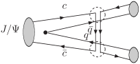
Figure 2: The hadronic loop diagram where the two hadrons inside the triangle are time-like, but virtual ones and the exchanged hadron possessing appropriate quantum numbers are also off-shell.

In fact, such a mechanism should also exist in all the decay modes of $J/\psi$ and make sizable contributions. In this work, we are going to evaluate the contribution from the hadronic loops where the intermediate hadrons are off-mass-shell.

The physical picture is following: $J/\psi$ first dissolves into two virtual hadrons, then by exchanging an appropriate hadron (i.e it possesses appropriate charge, flavor, spin and isospin) they turn into two on-shell real light hadrons which are to be seen by detector. The two intermediate hadrons are charmed hadrons, which contains flavor $c$ or $\bar{c}$, thus the transition $J/\psi\rightarrow H_{1}H_{2}$ where $H_{1}$ and $H_{2}$ are the two charmed hadrons, does not suffer from the OZI suppression. It is noted that the authors of Maiani discuss a possible mechanism for the relativistic heavy ion collision, where $J/\psi$ absorbs a pion existing in the hot environment to transit into two charmed mesons and the process may influence the observed $J/\psi$ suppression at RHIC. Even though such process is different from that under discussion of this work, the pictures have similarities.

In the practical calculations, the coupling constant of the effective vertex cannot be obtained by fitting data because such a process cannot occur due to the limited phase space. Then certain reasonable symmetries are invoked to get the coupling constants. We can argue that even though the coupling constant itself is not accurately determined, the qualitative conclusion is not seriously influenced.

In contrast with the derivation of the absorptive part of the triangle, the loop integration seems to be ultraviolet-divergent. In fact, following the standard procedure, the effective vertices are obtained from the chiral Lagrangian where all the concerned hadrons are on-shell, i.e. are real ones. To compensate the off-shell effects of the hadrons in the triangle, one may introduce form factors at each vertex. The form factors are inversely proportional to $(q^{2}-\Lambda^{2})$ where $\Lambda$ is a phenomenological parameter Anisowich which is expressed in terms of another phenomenological parameter $\alpha$ (see the following text for details). Because of existence of the form factors the ultraviolet divergence disappears, namely $\Lambda$ indeed plays a role similar to the cut-offs in the Pauli-Villas renormalization scheme Izukson ; peskin .

Picture is as follows, because, so far, we cannot derive the contribution from the OZI suppressed processes (i.e. via the three-gluon intermediate stage) to the total amplitude based on the quantum field theory yet, we denote such contribution by a phenomenological parameter $|\mathcal{G}_{S}^{PV}|$ which should be fixed by fitting data.

Therefore, by the simple picture, there are only two parameters, i.e. $\alpha$ and $|\mathcal{G}_{S}^{PV}|$. Concretely, we suppose that both the direct three-gluon process and hadronic loops contribute to the amplitude altogether, by fitting data of two distinict channels of $J/\psi\rightarrow PV$ where $P$ and $V$ stand for pseudoscalar and vector mesons respectively, we obtain the values of $\alpha$ and $|\mathcal{G}_{S}^{PV}|$ simultaneously. Here we choose to study processes $J/\psi\rightarrow PV$, since there are more data available. Of course when we derive $|\mathcal{G}_{S}^{PV}|$ from data, we have to carefully take care of the phase space of final states. Applying the obtained $\alpha$ and $|\mathcal{G}_{S}^{PV}|$, we evaluate the rates of other $J/\psi\rightarrow PV$ channels.

Indeed, our numerical results show that a destructive interference between the three-gluon process(OZI) and the hadronic loop can result in rates which are satisfactorily consistent with data. We will give a detailed discussion in the last section.

This work is organized as follows, after the introduction, in Sect. II, we formulate the hadronic loop contribution for $J/\psi\to PV$. In Sect. III, we present our numerical results along with all the input parameters. Finally, Sect. IV is devoted to discussion and conclusion.

II Formulation

The effective Lagrangian for $J/\psi$ decaying into light pseudoscalar and vector mesons is written as Chung

$$\mathcal{L} = (\mathcal{G}_{S}^{PV}+\mathcal{G}_{H}^{PV})\epsilon^{\mu\nu\alpha\beta}\epsilon_{\mu}Tr[\partial_{\nu}{\mathbb{P}}^{{\dagger}}\partial_{\beta}\mathbb{V}_{\alpha}]$$ (1)

$$+\mathcal{G}_{D}^{PV}\epsilon^{\mu\nu\alpha\beta}\epsilon_{\mu}Tr[\partial_{\nu}{\mathbb{P}}^{{\dagger}}]Tr[\partial_{\beta}\mathbb{V}_{\alpha}],$$

where $\mathcal{G}^{PV}_{{}_{S}}$, $\mathcal{G}^{PV}_{{}_{D}}$ and $\mathcal{G}^{PV}_{{}_{H}}$ respectively denote the effective couplings corresponding to single OZI diagram (Fig. 1 (a)), double OZI diagram (Fig. 1 (b)) and hadronic loop diagram (Fig. 2). In this work, we neglect the DOZI contribution. $\mathbb{P}$ and $\mathbb{V}$ respectively denote the nonet pseudoscalar and the nonet vector meson matrices

$$\mathbb{P} = \left(\begin{array}[]{ccc}\frac{\pi^{0}}{\sqrt{2}}+\frac{x_{\eta}\eta+x_{\eta^{\prime}}\eta^{\prime}}{\sqrt{2}}&\pi^{+}&K^{+}\\ \pi^{-}&-\frac{\pi^{0}}{\sqrt{2}}+\frac{x_{\eta}\eta+x_{\eta^{\prime}}\eta^{\prime}}{\sqrt{2}}&K^{0}\\ K^{-}&\bar{K}^{0}&y_{\eta}\eta+y_{\eta^{\prime}}\eta^{\prime}\end{array}\right),$$ (5)

$$\mathbb{V} = \left(\begin{array}[]{ccc}\frac{\rho^{0}}{\sqrt{2}}+\frac{\omega}{\sqrt{2}}&\rho^{+}&K^{*+}\\ \rho^{-}&-\frac{\rho^{0}}{\sqrt{2}}+\frac{\omega}{\sqrt{2}}&K^{*0}\\ K^{*-}&\bar{K}^{*0}&\phi\end{array}\right).$$ (9)

In the above expression, $x_{\eta,\eta^{\prime}}$ and $y_{\eta,\eta^{\prime}}$ describe the $\eta-\eta^{\prime}s$ mixing, and

$$x_{\eta}=y_{\eta^{\prime}}=\frac{\cos\theta-\sqrt{2}\sin\theta}{\sqrt{3}},\;\;\;x_{\eta^{\prime}}=-y_{\eta}=\frac{\sin\theta+\sqrt{2}\cos\theta}{\sqrt{3}},$$ (10)

where $\theta=-19.1^{\circ}$etamixing is the mixing angle of $\eta$ and $\eta^{\prime}$.

Taking $J/\psi\to\rho^{0}\pi^{0}$ as an example, we illustrate the calculations of the contributions from hadronic loops.

The Feynman diagrams describing the contributions of the hadronic loops to $J/\psi\to\rho^{0}\pi^{0}$ are depicted in Fig. 3. In the hadronic loops of diagrams (a)-(f) only $D^{(*)0}$ and $\bar{D}^{(*)0}$ are involved, but of course they can be simply replaced by $D^{(*)\pm}$ to compose new diagrams.

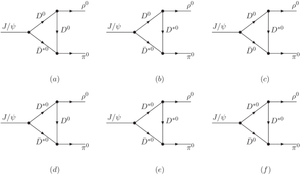
Figure 3: The Feynman diagrams which depict the decays of $J/\psi\to\rho^{0}\pi^{0}$ through $D^{(*)}$ hadronic loops.

In the former works lagrangian-hl ; Casalbuoni , the effective Lagrangians, which are related to our calculation, are constructed based on the chiral symmetry and heavy quark symmetry as

$$\mathcal{L} = ig_{{}_{J/\psi\mathcal{D}{\mathcal{D}}}}[{\mathcal{D}_{i}}{\stackrel{{\scriptstyle\leftrightarrow}}{{\partial}}}_{\mu}\mathcal{D}^{j{\dagger}}]\epsilon^{\mu}+g_{{}_{J/\psi\mathcal{D}{\mathcal{D}^{*}}}}\epsilon^{\mu\nu\alpha\beta}\epsilon_{\mu}\partial_{\nu}{\mathcal{D}_{i}}\partial_{\beta}{\mathcal{D}}^{*j{\dagger}}_{\alpha}$$ (11)

$$+ig_{{}_{J/\psi\mathcal{D^{*}}\mathcal{D^{*}}}}[{\mathcal{D^{*}}}_{i}^{\mu}(\partial_{\mu}\mathcal{D}^{*j{\dagger}}_{\nu})\epsilon^{\nu}-{\mathcal{D}^{*}}^{j\mu{\dagger}}(\partial_{\mu}{{\mathcal{D}}^{*}}_{i\nu})\epsilon^{\nu}-(\mathcal{D^{*}}^{\mu}_{i}{\stackrel{{\scriptstyle\leftrightarrow}}{{\partial}}}_{\nu}\mathcal{D}^{*j{\dagger}}_{\mu})\epsilon^{\nu}]$$

$$+\bigg{\{}\frac{1}{2}g_{{}_{\mathcal{D^{*}}\mathcal{D^{*}}\mathbb{P}}}\varepsilon_{\mu\nu\alpha\beta}\mathcal{D^{*}}_{i}^{\mu}\partial^{\nu}\mathbb{P}^{ij}{\stackrel{{\scriptstyle\leftrightarrow}}{{\partial}}}^{\alpha}\mathcal{D^{*}}_{j}^{\beta\dagger}-ig_{{}_{\mathcal{D^{*}}\mathcal{D}\mathbb{P}}}(\mathcal{D}^{i}\partial^{\mu}\mathbb{P}_{ij}\mathcal{D^{*}}_{\mu}^{j\dagger}-\mathcal{D^{*}}_{\mu}^{i}\partial^{\mu}\mathbb{P}_{ij}\mathcal{D}^{j\dagger})$$

$$-ig_{{}_{\mathcal{D}\mathcal{D}\mathbb{V}}}\mathcal{D}_{i}^{\dagger}{\stackrel{{\scriptstyle\leftrightarrow}}{{\partial}}}_{\mu}\mathcal{D}^{j}(\mathbb{V}^{\mu})^{i}_{j}-2f_{{}_{\mathcal{D^{*}}\mathcal{D}\mathbb{V}}}\varepsilon_{\mu\nu\alpha\beta}(\partial^{\mu}\mathbb{V}^{\nu})^{i}_{j}(\mathcal{D}_{i}^{\dagger}{\stackrel{{\scriptstyle\leftrightarrow}}{{\partial}}}^{\alpha}\mathcal{D^{*}}^{\beta j}-\mathcal{D^{*}}_{i}^{\beta\dagger}{\stackrel{{\scriptstyle\leftrightarrow}}{{\partial}}}^{\alpha}\mathcal{D}^{j})$$

$$+ig_{{}_{\mathcal{D^{*}}\mathcal{D^{*}}\mathbb{V}}}\mathcal{D^{*}}_{i}^{\nu\dagger}{\stackrel{{\scriptstyle\leftrightarrow}}{{\partial}}}_{\mu}\mathcal{D^{*}}_{\nu}^{j}(\mathbb{V}^{\mu})^{i}_{j}+4if_{{}_{\mathcal{D^{*}}\mathcal{D^{*}}\mathbb{V}}}\mathcal{D^{*}}_{i\mu}^{\dagger}(\partial^{\mu}\mathbb{V}^{\nu}-\partial^{\nu}\mathbb{V}^{\mu})^{i}_{j}\mathcal{D^{*}}_{\nu}^{j}\bigg{\}},$$

where $\mathcal{D}$ and $\mathcal{D^{*}}$ are respectively pseudoscalar and vector heavy mesons, i.e. $\mathcal{D^{(*)}}$=(($\bar{D}^{0})^{(*)}$, $(D^{-})^{(*)}$, $(D_{s}^{-})^{(*)}$). The actual values of the coupling constants will be given in the following section.

With these Lagrangians, we write out the decay amplitudes of $J/\psi\rightarrow\rho^{0}\pi^{0}$. For Fig. 3 (a),

$$\mathcal{M}_{a} = \mathcal{A}_{\rho^{0}\pi^{0}}\int\frac{d^{4}q}{(2\pi)^{4}}[ig_{J/\psi DD^{*}}\varepsilon_{\mu\nu\alpha\beta}\epsilon_{J/\psi}^{\mu}(ip_{2}^{\nu})(ip_{1}^{\beta})][ig_{DD\rho}(-p_{1}-q)\cdot\epsilon_{\rho}][g_{D^{*}D\pi}(ip_{4\sigma})]$$ (12)

$$\times\frac{i}{p_{1}^{2}-m_{D}^{2}}\frac{i(-g^{\alpha\sigma})}{p_{2}^{2}-m_{D^{*}}^{2}}\frac{i}{q^{2}-m_{D}^{2}}\mathcal{F}^{2}(m_{D},q^{2}).$$

For saving the space, we collect the concrete expressions of the amplitudes corresponding to Fig. 3 (b)-(f) in the Appendix.

In the amplitudes, $\mathcal{A}_{\rho^{0}\pi^{0}}=1/2$. $\mathcal{F}(m_{i},q^{2})$s represent the form factors which compensate the off-shell effects of the mesons at the vertices and are written as formfactor-pv

$$\mathcal{F}(m_{i},q^{2})=\frac{\Lambda^{2}-m_{i}^{2}}{\Lambda^{2}-q^{2}}$$ (13)

where $\Lambda$ is a phenomenological parameter. It is obvious that as $q^{2}\rightarrow 0$ it becomes a number and if $\Lambda\gg m_{i}$, it turns to be unity. Whereas, as $q^{2}\rightarrow\infty$, the form factor approaches to zero. In that situation, the distance becomes very small, so that the inner structure would manifest itself and the whole picture of hadron interaction is no longer valid. At that region the form factor turns to zero and plays a role to cut off the end effect. The concrete expression of $\Lambda$ is represented as HY-Chen

$$\Lambda(m_{i})=m_{i}+\alpha\Lambda_{QCD},$$ (14)

where $m_{i}$ denotes the mass of exchanged meson. $\Lambda_{QCD}=220$ MeV. $\alpha$ is a phenomenological parameter. In fact, in literature, some other forms for the form factors are suggestedform-factor , all of them depend on phenomenological parameters which are obtained by fitting data, therefore in the calculations all the forms are somehow equivalent even though some of them may provide a better convergent behavior for the triangle loop integration. That is very similar to the case of the pauli-Villas renormalization scheme Izukson ; peskin .

Taking Fig. 3 (a) as an example, we carry out the Feynman parameter integration for (12) and get

$$\mathcal{M}_{(a)} = \mathcal{A}_{\rho^{0}\pi^{0}}g_{{}_{J/\psi DD^{*}}}g_{{}_{DD\rho}}g_{{}_{D^{*}D\pi}}\int^{1}_{0}dx\int^{1-x}_{0}dy\bigg{[}\frac{2}{(4\pi)^{2}}\log\Big{(}\frac{\Delta(m_{{}_{D}},m_{{}_{D^{*}}},\Lambda(m_{{}_{D}}))}{\Delta(m_{{}_{D}},m_{{}_{D^{*}}},m_{{}_{D}})}\Big{)}$$ (15)

$$-\frac{(\Lambda^{2}-m_{D}^{2})y}{8\pi^{2}\Delta(m_{{}_{D}},m_{{}_{D^{*}}},m_{{}_{D}})}\bigg{]}(-2\varepsilon_{\mu\nu\alpha\beta}\epsilon_{J/\psi}^{\mu}\epsilon_{\rho}^{\nu}p_{3}^{\alpha}p_{4}^{\beta}),$$

where

$$\Delta(a,b,c) = m_{3}^{2}(1-x-y)^{2}-2(p_{3}\cdot p_{4})(1-x-y)x+m_{4}^{2}x^{2}-(m_{3}^{2}-a^{2})(1-x-y)$$

$$-(m_{4}^{2}-b^{2})x+yc^{2},$$

$m_{3}$($m_{4}$), $p_{3}$($p_{4}$) are the masses and four- momenta of $\rho^{0}$($\pi^{0}$) respectively. Because of the form factors, the ultraviolet divergence does not exist as expected.

We use the same method to deal with the amplitudes corresponding to Fig. 3 (b)-(f) and also put them in the appendix.

To obtain the amplitudes corresponding to hadronic loops which contain $D^{(*)\pm}$, one only needs to replace the parameters corresponding to $D^{(*)0}$ and $\bar{D}^{(*)0}$ by that to $D^{(*)+}$ and $D^{(*)-}$ in the above six expressions (15)-(33). Thus contribution from the hadronic loops to the total amplitude can be eventually expressed as

$$\mathcal{M}^{\rho^{0}\pi^{0}}_{H} = (\mathcal{M}_{a}+\mathcal{M}_{b}+\mathcal{M}_{c}+\mathcal{M}_{d}+\mathcal{M}_{e}+\mathcal{M}_{f})$$ (16)

$$+(\mathcal{M}_{a}+\mathcal{M}_{b}+\mathcal{M}_{c}+\mathcal{M}_{d}+\mathcal{M}_{e}+\mathcal{M}_{f})|_{m_{D^{(*)0}}\to m_{D^{(*)\pm}}}$$

$$= \mathcal{G}^{{\rho^{0}\pi^{0}}}_{{}_{H}}(\alpha)\varepsilon_{\mu\nu\alpha\beta}\epsilon_{J/\psi}^{\mu}\epsilon_{\rho}^{\nu}p_{3}^{\alpha}p_{4}^{\beta},$$

where $\mathcal{G}^{{\rho^{0}\pi^{0}}}_{{}_{H}}(\alpha)$ denotes the effective coupling for $J/\psi\to\rho^{0}\pi^{0}$ induced by the hadronic loops where $\mathcal{G}^{{\rho^{0}\pi^{0}}}_{{}_{H}}(\alpha)$ is a function of variable $\alpha$.

Similar to $J/\psi\to\rho^{0}\pi^{0}$, we can also obtain contributions of hadronic loops to $J/\psi\to K^{*+}K^{-}+\mathrm{c.c.},\;K^{*0}\bar{K}^{0}+\mathrm{c.c.},\;\omega\eta^{(^{\prime})},\;\phi\eta^{(^{\prime})}$. It is noticed that the hadronic loops for processes $J/\psi\to K^{*+}K^{-}+\mathrm{c.c.},\;K^{*0}\bar{K}^{0}+\mathrm{c.c.},\;\phi\eta^{(^{\prime})}$ include $D_{s}^{(*)(\pm)}$ mesons and in the calculations, the coefficient $\mathcal{A}_{\rho^{0}\pi^{0}}$ is replaced by $\mathcal{A}_{K^{*}K}=1$ (or $\mathcal{A}_{\omega\eta^{(^{\prime})}}=x_{\eta^{(^{\prime})}}/2,\;\mathcal{A}_{\phi\eta^{(^{\prime})}}=y_{\eta^{(^{\prime})}}/2$).

We have obtained seven quantities which contain both contributions of the OZI process and the hadronic loop

$$\mathcal{G}^{\rho^{0}\pi^{0}} = \mathcal{G}^{PV}_{S}\beta^{\rho^{0}\pi^{0}}+\mathcal{G}^{\rho^{0}\pi^{0}}_{H}(\alpha),$$ (17)

$$\mathcal{G}^{K^{*+}K^{-}} = \mathcal{G}^{PV}_{S}\beta^{K^{*+}K^{-}}+\mathcal{G}^{K^{*+}K^{-}}_{H}(\alpha),$$ (18)

$$\mathcal{G}^{\omega\eta} = \mathcal{G}^{PV}_{S}\beta^{\omega\eta}+\mathcal{G}^{\omega\eta}_{D}+\mathcal{G}^{\omega\eta}_{H}(\alpha),$$ (19)

$$\mathcal{G}^{\omega\eta^{\prime}} = \mathcal{G}^{PV}_{S}\beta^{\omega\eta^{\prime}}+\mathcal{G}^{\omega\eta^{\prime}}_{D}+\mathcal{G}^{\omega\eta^{\prime}}_{H}(\alpha),$$ (20)

$$\mathcal{G}^{\phi\eta} = \mathcal{G}^{PV}_{S}\beta^{\phi\eta}+\mathcal{G}^{\phi\eta}_{D}+\mathcal{G}^{\phi\eta}_{H}(\alpha),$$ (21)

$$\mathcal{G}^{\phi\eta^{\prime}} = \mathcal{G}^{PV}_{S}\beta^{\phi\eta^{\prime}}+\mathcal{G}^{\phi\eta^{\prime}}_{D}+\mathcal{G}^{\phi\eta^{\prime}}_{H}(\alpha),$$ (22)

where the contributions from the DOZI processes are ignored, i.e. one can set $\mathcal{G}^{\omega\eta^{(^{\prime})}}_{D}=\mathcal{G}^{\phi\eta^{(^{\prime})}}_{D}=0$. Geometry factors $\beta^{PV}$ satisfy the following relation:

$$\beta^{\rho^{0}\pi^{0}}_{S}:\beta^{K^{*+}K^{-}}_{S}:\beta^{\omega\eta}_{S}:\beta^{\omega\eta^{\prime}}_{S}:\beta^{\phi\eta}_{S}:\beta^{\phi\eta^{\prime}}_{S}=1:{1}:x_{\eta}:x_{\eta^{\prime}}:y_{\eta}:y_{\eta^{\prime}}.$$ (23)

The SU(3) geometry factors $\beta^{PV}$ is obtained by taking the trace $Tr(PV)$ as $J/\psi$ is an SU(3) singlet, and in fact, it is just the SU(3) C-G coefficient for the concerned channel.

Thus using eqs. (17) and (18), the parameter $\alpha$ is determined. With it, we are able to calculate the values of $\mathcal{G}^{PV}_{H}$.

III Numerical results

Because of the flavor SU(3) symmetry, it is reasonable to set $g_{{}_{J/\psi D_{s}\bar{D}_{s}}}\approx g_{{}_{J/\psi D\bar{D}}}$. Based on the naive vector dominance model and using the data of the branching ratio of $J/\psi\to e^{+}e^{-}$, the authors of Ref. Achasov determined ${g_{{}_{J/\psi D\bar{D}}}^{2}}/{(4\pi)}=5$. As a consequence of the spin symmetry in the HQET, $g_{{}_{J/\psi D_{s}\bar{D}_{s}^{*}}}$ and $g_{{}_{J/\psi D_{s}^{*}\bar{D}_{s}^{*}}}$ satisfy the relations: $g_{{}_{J/\psi D_{s}\bar{D}_{s}^{*}}}={g_{{}_{J/\psi D\bar{D}_{s}}}}/{m_{{}_{D_{s}}}}$ and $g_{{}_{J/\psi D^{*}_{s}\bar{D}_{s}^{*}}}=g_{{}_{J/\psi D_{s}\bar{D}_{s}}}$ JPsi-relation . Other coupling constants related to $J/\psi\to PV$ include HY-Chen :

$$g_{{}_{D^{*}D^{*}\pi}} = \frac{g_{{}_{D^{*}D\pi}}}{\sqrt{m_{{}_{D}}m_{{}_{D^{*}}}}}=\frac{2g}{f_{\pi}},\;\;\;g_{{}_{DDV}}=g_{{}_{D^{*}D^{*}V}}=\frac{\beta g_{{}_{V}}}{\sqrt{2}},\;\;\;f_{{}_{D^{*}DV}}=\frac{f_{{}_{D^{*}D^{*}V}}}{m_{{}_{D^{*}}}}=\frac{\lambda g_{{}_{V}}}{\sqrt{2}},$$

$$g_{{}_{D^{*}D_{s}K}} = \sqrt{\frac{m_{{}_{D_{s}}}}{m_{{}_{D}}}}g_{{}_{D^{*}D\pi}},\;\;\;g_{{}_{D_{s}^{*}DK}}=\sqrt{\frac{m_{{}_{D_{s}^{*}}}}{m_{{}_{D^{*}}}}}g_{{}_{D^{*}D\pi}},\;\;\;g_{{}_{V}}=\frac{m_{{}_{\rho}}}{f_{\pi}},$$

where $f_{\pi}=132$ MeV, $g_{{}_{V}},\;\beta$ and $\lambda$ are parameters in the effective chiral Lagrangian that describes the interaction of heavy mesons with low-momentum light vector mesons Casalbuoni . Following ref. Isola , we take $g=0.59$, $\beta=0.9$ and $\lambda=0.56$ $\mathrm{GeV}^{-1}$. Meanwhile, the coupling constants $g_{D_{s}^{(*)}D_{s}^{(*)}\phi(K^{*})}$($f_{D_{s}^{(*)}D_{s}^{(*)}\phi(K^{*})}$) are related to $g_{D^{(*)}D^{(*)}\rho}$($f_{D^{(*)}D^{(*)}\rho}$) and one can expect the relations in the limit of SU(3) symmetry HY-Chen

$$g_{D_{s}^{(*)}D_{s}^{(*)}\phi} = \frac{m_{D_{s}^{(*)}}}{m_{D^{(*)}}}g_{D^{(*)}D^{(*)}\rho},\;\;\;f_{D_{s}^{(*)}D_{s}^{(*)}\phi}=\frac{m_{D_{s}^{(*)}}}{m_{D^{(*)}}}f_{D^{(*)}D^{(*)}\rho},$$

$$g_{D^{(*)}D_{s}^{(*)}K^{*}} = \sqrt{\frac{m_{D_{s}^{(*)}}}{m_{D^{(*)}}}}g_{D^{(*)}D^{(*)}\rho},\;\;\;f_{D^{(*)}D_{s}^{(*)}K^{*}}=\sqrt{\frac{m_{D_{s}^{(*)}}}{m_{D^{(*)}}}}f_{D^{(*)}D^{(*)}\rho}.$$

Using eqs. (17) and (18), we have determined $\alpha$ and $\mathcal{G}^{PV}_{S}$ as

$$\alpha=0.13,\;\;\;|\mathcal{G}^{PV}_{S}|=4.51.$$

Namely, in our scheme, the hadronic loop contribution to $J/\psi\to PV$ is theoretically calculated whereas the OZI contribution is obtained by fitting the data of the two channels. The obtained $|\mathcal{G}^{PV}_{S}|=4.51$ is supposed to be universal for all channels of $J/\psi\to PV$ based on SU(3) symmetry. With eqs. (19)-(22), we predict the values of $\mathcal{G}^{PV}$ for all channels of $J/\psi\to PV$. The obtained results are listed in Table. 1.

Decay mode	$\rho^{0}\pi^{0}$	$K^{*+}K^{-}+c.c.$	$\phi\eta$	$\phi\eta^{\prime}$	$\omega\eta$	$\omega\eta^{\prime}$
BR$\times 10^{-3}$(Experiment)PDG	$4.2\pm 0.5$	$5.0\pm 0.4$	$0.65\pm 0.07$	$0.33\pm 0.04$	$1.58\pm 0.16$	$0.167\pm 0.025$
$\mathcal{G}^{PV}(10^{-3}$ GeV${}^{-1})$	$2.08\pm 0.25$	$1.65\pm 0.26$	$0.89\pm 0.096$	$0.71\pm 0.086$	$1.27\pm 0.13$	$0.46\pm 0.069$
$\mathcal{G}^{PV}_{H}(10^{-3}$GeV${}^{-1})$(Theory)	6.59	6.16	3.55	5.13	5.46	4.07
$\mathcal{G}^{PV}(10^{-3}$GeV${}^{-1})$(Theory)	2.08(fitting)	1.65(fitting)	0.92	0.62	0.95	0.40
BR$\times 10^{-3}$(Theory)	4.2(fitting)	5.0(fitting)	0.70	0.25	0.86	0.14

Table 1: The first two modes are well measured, we obtain $\alpha$ and $|\mathcal{G}^{PV}_{S}|=4.51$ by fitting them.

IV conclusion and discussion

From above discussions and numerical results, one has the following observations.

(1) The contribution from the hadronic loops is sizable and has the same order of magnitude as that from the SOZI process.

(2) To get reasonable results which are consistent with data, the interference between the SOZI contribution and that from hadronic loops is destructive.

(3) We derive the parameter $\alpha$ and the universal $|\mathcal{G}^{PV}_{S}|$ by fitting data of the first two distinct modes of $J/\psi$ and present in the first two columns of table 1. In our picture, there are only two free parameters. The values of $\mathcal{G}^{PV}$ which we predict in terms of $\alpha$ and $\mathcal{G}^{PV}_{H}$ are reasonably consistent with the experimental data.

In this work, we rely on two key assumptions. The first is that the value $|\mathcal{G}^{PV}_{S}|$ is universal for all channels of $J/\psi\rightarrow PV$ due to the flavor-blindness of gluon coupling to quarks. This treatment is similar to that made Maiani for study process $\pi+J/\psi\rightarrow D^{(*)}+D^{(*)}$ in a hot RHIC environment.

In this work, we re-parameterize $\Lambda$ in terms of $\alpha$ following the ansatz suggested by the authors of Ref. HY-Chen . It seems that one may gain some information about the parameter $\alpha$ from the FSI calculations Anisowich ; Cheng , however, it is not really the case. Even though in both calculations, one deals with the triangle diagrams which are composed of only hadrons, the situations are different. For FSI, one calculates the absorptive part where only the exchanged meson is off-shell, whereas for the calculation of the dispersive part, all the three mesons in the triangle are off-shell. Form factors are phenomenologically introduced to compensate the off-shell effects at each vertex, thus the form factors should not be the same for calculating the dispersive and absorptive parts, i.e. even though they have the same expressions, the involved free parameters may be different. It is noted that in the FSI case, the value of $\alpha$ in the form factor is expected to be of order unity HY-Chen , but in the case of hadronic loop the value of $\alpha$ is obviously smaller. In our strategy, we do not priori set its value, but let data determine it.

As our conclusion, it is obvious that the contribution from the hadronic loop to $J/\psi\to\;two\;light\;mesons$ should exist. The question is how large it is compared to that of the SOZI processes. Namely, if only the SOZI process is responsible for the decays of $J/\psi$, it is hard to explain the data and as the contribution from the hadronic loops being added, one can see that the data are well accommodated within a tolerable range. In our scenario, there are only two parameters in the whole scenario and they are determined by fitting data of two channels. With these two parameters, we evaluate the branching ratios of the other channels of $J/\psi\rightarrow PV$ and the theoretical predictions are consistent with data. It indicates that the ansatz is reasonable and the whole picture makes sense. Indeed, there is only one channel, i.e. $J/\psi\rightarrow\omega\eta$, for which the theoretical prediction on the branching ratio is about 0.6 of the experimental data. Even though there exists such a discrepancy, for a rough estimate the consistency is not bad at all and we would like to urge our experimental colleagues to redo the measurement to get more accurate results. On the other side, so far the SOZI processes have not well calculated in the framework of quantum field theory yet, we also need to complete such a derivation and detect the value which we obtained by fitting data and assuming a universality for all modes. To be more accurate, however, further theoretical and experimental efforts may be needed. This mechanism should exist not only for $J/\psi$ exclusive decays, but also for other members of charmonia. However, for higher excited states of chamonia, the channels with final states composed of charmed hadrons are open, and the situation becomes more complicated. This picture also applies to the $\Upsilon$ decays and can be tested by the future experimental data.

Appendix

One obtains the decay amplitudes of $J/\psi\to\rho^{0}\pi^{0}$ corresponding to Fig. 3 (b)-(f).

For Fig. 3 (b),

$$\mathcal{M}_{b} = \mathcal{A}_{\rho^{0}\pi^{0}}\int\frac{d^{4}q}{(2\pi)^{4}}[ig_{J/\psi DD^{*}}\varepsilon_{\mu\nu\alpha\beta}\epsilon_{J/\psi}^{\mu}(ip_{2}^{\nu})(ip_{1}^{\beta})][-{2i}f_{D^{*}D\rho}\varepsilon^{\kappa\xi\lambda\tau}(ip_{3}^{\kappa})\epsilon_{\rho}^{\xi}(-ip_{1}^{\lambda}-iq^{\lambda})]$$ (24)

$$\times[ig_{D^{*}D^{*}\pi}\varepsilon_{\pi\zeta\delta\omega}(ip_{4}^{\zeta})(-ip_{2}^{\delta})]\frac{i}{p_{1}^{2}-m_{D}^{2}}\frac{i(-g^{\alpha\pi})}{p_{2}^{2}-m_{D^{*}}^{2}}\frac{i(-g^{\tau\omega})}{q^{2}-m_{D^{*}}^{2}}\mathcal{F}^{2}(m_{D^{*}},q^{2}).$$

For Fig. 3 (c),

$$\mathcal{M}_{c} = \mathcal{A}_{\rho^{0}\pi^{0}}\int\frac{d^{4}q}{(2\pi)^{4}}[ig_{J/\psi DD}(p_{1}-p_{2})\cdot\epsilon_{J/\psi}][-2if_{D^{*}D\rho}\varepsilon^{\kappa\xi\tau\lambda}(ip_{3}^{\kappa})\epsilon_{\rho}^{\xi}(-ip_{1}^{\lambda}-iq^{\lambda})]$$ (25)

$$\times[g_{D^{*}D\pi}(ip_{4}^{\mu})]\frac{i}{p_{1}^{2}-m_{D}^{2}}\frac{i}{p_{2}^{2}-m_{D}^{2}}\frac{i(-g_{\mu\tau})}{q^{2}-m_{D^{*}}^{2}}\mathcal{F}^{2}(m_{D^{*}},q^{2}).$$

For Fig. 3 (d),

$$\mathcal{M}_{d} = \mathcal{A}_{\rho^{0}\pi^{0}}\int\frac{d^{4}q}{(2\pi)^{4}}\{g_{J/\psi D^{*}D^{*}}[ip_{1}^{\nu}\epsilon_{J/\psi}^{\mu}-ip_{2}^{\mu}\epsilon_{J/\psi}^{\nu}-i(p_{2}-p_{1})\cdot\epsilon_{J/\psi}g^{\mu\nu}]\}$$ (26)

$$\times[2if_{D^{*}D\rho}\varepsilon_{\pi\zeta\delta\omega}(ip_{3}^{\pi})\epsilon_{\rho}^{\zeta}(-ip_{1}^{\delta}-iq^{\delta})][g_{D^{*}D\pi}(ip_{4}^{\alpha})]$$

$$\times\frac{i(-g_{\mu}^{\omega})}{p_{1}^{2}-m_{D^{*}}^{2}}\frac{i(-g_{\nu\alpha})}{p_{2}^{2}-m_{D^{*}}^{2}}\frac{i}{q^{2}-m_{D}^{2}}\mathcal{F}^{2}(m_{D},q^{2}).$$

For Fig. 3 (e),

$$\mathcal{M}_{e} = \mathcal{A}_{\rho^{0}\pi^{0}}\int\frac{d^{4}q}{(2\pi)^{4}}\{g_{J/\psi D^{*}D^{*}}[ip_{1}^{\nu}\epsilon_{J/\psi}^{\mu}-ip_{2}^{\mu}\epsilon_{J/\psi}^{\nu}-i(p_{2}-p_{1})\cdot\epsilon_{J/\psi}g^{\mu\nu}]\}$$ (27)

$$\times\{-g_{D^{*}D^{*}\rho}(-ip_{1}-iq)\cdot\epsilon_{\rho}g^{\alpha\beta}-4f_{D^{*}D^{*}\rho}(ip_{3}^{\alpha}\epsilon_{\rho}^{\beta}-ip_{3}^{\beta}\epsilon_{\rho}^{\alpha})\}$$

$$\times[ig_{D^{*}D^{*}\pi}\varepsilon_{\pi\zeta\delta\omega}(ip_{4}^{\zeta})(-ip_{2}^{\delta})]\frac{i(-g_{\mu\alpha})}{p_{1}^{2}-m_{D^{*}}^{2}}\frac{i(-g^{\nu\pi})}{p_{2}^{2}-m_{D^{*}}^{2}}\frac{i(-g_{\beta}^{\omega})}{q^{2}-m_{D^{*}}^{2}}\mathcal{F}^{2}(m_{D^{*}},q^{2}).$$

For Fig. 3 (f),

$$\mathcal{M}_{f} = \mathcal{A}_{\rho^{0}\pi^{0}}\int\frac{d^{4}q}{(2\pi)^{4}}[ig_{J/\psi DD^{*}}\varepsilon_{\mu\nu\alpha\beta}\epsilon_{J/\psi}^{\mu}(ip_{2}^{\nu})(ip_{1}^{\beta})]$$ (28)

$$\times\{-g_{D^{*}D^{*}\rho}(-ip_{1}-iq)\cdot\epsilon_{\rho}g^{\delta\tau}-4f_{D^{*}D^{*}\rho}(ip_{3}^{\delta}\epsilon_{\rho}^{\tau}-ip_{3}^{\tau}\epsilon_{\rho}^{\delta})\}$$

$$\times[g_{D^{*}D\pi}(ip_{4}^{\kappa})]\frac{i(-g^{\alpha}_{\delta})}{p_{1}^{2}-m_{D^{*}}^{2}}\frac{i}{p_{2}^{2}-m_{D}^{2}}\frac{i(-g_{\tau\kappa})}{q^{2}-m_{D^{*}}^{2}}\mathcal{F}^{2}(m_{D^{*}},q^{2}).$$

By further calculations, we obtain

$$\mathcal{M}_{(b)} = \mathcal{A}_{\rho^{0}\pi^{0}}g_{{}_{J/\psi DD^{*}}}2f_{{}_{DD^{*}\rho}}g_{{}_{D^{*}D^{*}\pi}}\int^{1}_{0}dx\int^{1-x}_{0}dy\bigg{\{}\Big{[}\frac{(\Lambda^{2}-m_{D^{*}}^{2})y}{16\pi^{2}\Delta^{2}(m_{{}_{D}},m_{{}_{D^{*}}},\Lambda(m_{{}_{D^{*}}}))}$$ (29)

$$-\frac{1}{16\pi^{2}\Delta(m_{{}_{D}},m_{{}_{D^{*}}},m_{{}_{D^{*}}})}+\frac{1}{16\pi^{2}\Delta(m_{{}_{D}},m_{{}_{D^{*}}},\Lambda(m_{{}_{D^{*}}}))}\Big{]}\Big{[}-2xy^{2}(p_{3}\cdot p_{4})^{2}$$

$$-2x^{2}y(p_{3}\cdot p_{4})^{2}+2xy(p_{3}\cdot p_{4})^{2}+2xy^{2}m_{3}^{2}m_{4}^{2}+2x^{2}ym_{3}^{2}m_{4}^{2}-2xym_{3}^{2}m_{4}^{2}\Big{]}$$

$$+\bigg{[}\frac{2}{(4\pi)^{2}}\log\Big{(}\frac{\Delta(m_{{}_{D}},m_{{}_{D^{*}}},\Lambda(m_{{}_{D^{*}}}))}{\Delta(m_{{}_{D}},m_{{}_{D^{*}}},m_{{}_{D^{*}}})}\Big{)}-\frac{(\Lambda^{2}-m_{D^{*}}^{2})y}{8\pi^{2}\Delta(m_{{}_{D}},m_{{}_{D^{*}}},m_{{}_{D^{*}}})}\bigg{]}$$

$$\times\Big{[}(-6y-2x+1)(p_{3}\cdot p_{4})+2m_{3}^{2}-2m_{3}^{2}x-2m_{3}^{2}y+2y(p_{3}\cdot p_{4})\Big{]}\bigg{\}}$$

$$\times\varepsilon_{\mu\nu\alpha\beta}\epsilon_{J/\psi}^{\mu}\epsilon_{\rho}^{\nu}p_{3}^{\alpha}p_{4}^{\beta},$$

$$\mathcal{M}_{(c)} = \mathcal{A}_{\rho^{0}\pi^{0}}g_{{}_{J/\psi DD}}f_{{}_{DD^{*}\rho}}g_{{}_{DD^{*}\pi}}\int^{1}_{0}dx\int^{1-x}_{0}dy\bigg{[}\frac{2}{(4\pi)^{2}}\log\Big{(}\frac{\Delta(m_{{}_{D}},m_{{}_{D}},\Lambda(m_{{}_{D^{*}}}))}{\Delta(m_{{}_{D}},m_{{}_{D}},m_{{}_{D^{*}}})}\Big{)}$$ (30)

$$-\frac{(\Lambda^{2}-m_{D^{*}}^{2})y}{8\pi^{2}\Delta(m_{{}_{D}},m_{{}_{D}},m_{{}_{D^{*}}})}\bigg{]}\Big{[}-8\varepsilon_{\mu\nu\alpha\beta}\epsilon_{J/\psi}^{\mu}\epsilon_{\rho}^{\nu}p_{3}^{\alpha}p_{4}^{\beta}\Big{]},$$

$$\mathcal{M}_{(d)} = \mathcal{A}_{\rho^{0}\pi^{0}}g_{{}_{J/\psi D^{*}D^{*}}}f_{{}_{DD^{*}\rho}}g_{{}_{D^{*}D\pi}}\int^{1}_{0}dx\int^{1-x}_{0}dy\bigg{\{}\Big{[}\frac{(\Lambda^{2}-m_{D}^{2})y}{16\pi^{2}\Delta^{2}(m_{{}_{D^{*}}},m_{{}_{D^{*}}},\Lambda(m_{{}_{D}}))}$$ (31)

$$-\frac{1}{16\pi^{2}\Delta(m_{{}_{D^{*}}},m_{{}_{D^{*}}},m_{{}_{D}})}+\frac{1}{16\pi^{2}\Delta(m_{{}_{D^{*}}},m_{{}_{D^{*}}},\Lambda(m_{{}_{D}}))}\Big{]}\Big{[}4x^{2}m_{4}^{2}+4x^{2}(p_{3}\cdot p_{4})$$

$$+4xy(p_{3}\cdot p_{4})\Big{]}+12\bigg{[}\frac{2}{(4\pi)^{2}}\log\Big{(}\frac{\Delta(m_{{}_{D^{*}}},m_{{}_{D^{*}}},\Lambda(m_{{}_{D}}))}{\Delta(m_{{}_{D^{*}}},m_{{}_{D^{*}}},m_{{}_{D}})}\Big{)}-\frac{(\Lambda^{2}-m_{D}^{2})y}{8\pi^{2}\Delta(m_{{}_{D^{*}}},m_{{}_{D^{*}}},m_{{}_{D}})}\bigg{]}\bigg{\}}$$

$$\times\varepsilon_{\mu\nu\alpha\beta}\epsilon_{J/\psi}^{\mu}\epsilon_{\rho}^{\nu}p_{3}^{\alpha}p_{4}^{\beta},$$

$$\mathcal{M}_{(e)} = \mathcal{A}_{\rho^{0}\pi^{0}}g_{{}_{J/\psi D^{*}D^{*}}}g_{{}_{D^{*}D^{*}\pi}}\int^{1}_{0}dx\int^{1-x}_{0}dy\bigg{\{}\Big{[}\frac{(\Lambda^{2}-m_{D^{*}}^{2})y}{16\pi^{2}\Delta^{2}(m_{{}_{D^{*}}},m_{{}_{D^{*}}},\Lambda(m_{{}_{D^{*}}}))}$$ (32)

$$-\frac{1}{16\pi^{2}\Delta(m_{{}_{D^{*}}},m_{{}_{D^{*}}},m_{{}_{D^{*}}})}+\frac{1}{16\pi^{2}\Delta(m_{{}_{D^{*}}},m_{{}_{D^{*}}},\Lambda(m_{{}_{D^{*}}}))}\Big{]}f_{{}_{D^{*}D^{*}\rho}}\Big{[}4x^{2}m_{3}^{2}$$

$$+4y^{2}m_{3}^{2}+4m_{3}^{2}-8xm_{3}^{2}-8ym_{3}^{2}+8xym_{3}^{2}+4x^{2}(p_{3}\cdot p_{4})+4(p_{3}\cdot p_{4})$$

$$-8x(p_{3}\cdot p_{4})-4y(p_{3}\cdot p_{4})+4xy(p_{3}\cdot p_{4})\Big{]}+\bigg{[}\frac{2}{(4\pi)^{2}}\log\Big{(}\frac{\Delta(m_{{}_{D^{*}}},m_{{}_{D^{*}}},\Lambda(m_{{}_{D^{*}}}))}{\Delta(m_{{}_{D^{*}}},m_{{}_{D^{*}}},m_{{}_{D^{*}}})}\Big{)}$$

$$-\frac{(\Lambda^{2}-m_{D^{*}}^{2})y}{8\pi^{2}\Delta(m_{{}_{D^{*}}},m_{{}_{D^{*}}},m_{{}_{D^{*}}})}\bigg{]}[16f_{{}_{D^{*}D^{*}\rho}}-2g_{{}_{D^{*}D^{*}\rho}}]\bigg{\}}\varepsilon_{\mu\nu\alpha\beta}\epsilon_{J/\psi}^{\mu}\epsilon_{\rho}^{\nu}p_{3}^{\alpha}p_{4}^{\beta},$$

$$\mathcal{M}_{(f)} = \mathcal{A}_{\rho^{0}\pi^{0}}g_{{}_{J/\psi D^{*}D}}f_{{}_{D^{*}D^{*}\rho}}g_{{}_{DD^{*}\pi}}\int^{1}_{0}dx\int^{1-x}_{0}dy\bigg{\{}\Big{[}\frac{(\Lambda^{2}-m_{D^{*}}^{2})y}{16\pi^{2}\Delta^{2}(m_{{}_{D^{*}}},m_{{}_{D}},\Lambda(m_{{}_{D^{*}}}))}$$ (33)

$$-\frac{1}{16\pi^{2}\Delta(m_{{}_{D^{*}}},m_{{}_{D}},m_{{}_{D^{*}}})}+\frac{1}{16\pi^{2}\Delta(m_{{}_{D^{*}}},m_{{}_{D}},\Lambda(m_{{}_{D^{*}}}))}\Big{]}\Big{[}-4y(p_{3}\cdot p_{4})\Big{]}\bigg{\}}$$

$$\times\varepsilon_{\mu\nu\alpha\beta}\epsilon_{J/\psi}^{\mu}\epsilon_{\rho}^{\nu}p_{3}^{\alpha}p_{4}^{\beta}.$$

References

• (1) S. Okubo, Phys. Lett. 5, 165 (1963); G. Zweig, CERN Rep. 8419/TH-412; CERN Preprints TH-401, TH-412; J. Iizuka, Prog. Theor. Phys. Suppl. 37/38, 21 (1966).
• (2) Mark II Collaboration, M. Franklin et al, Phys. Rev. Lett. 51, 963 (1983); BES Collaboration, J. Z. Bai et al., Phys. Rev. D54, 1221 (1996).
• (3) J. L. Rosner, Phys. Rev. D64, 094002 (2001).
• (4) V.V. Anisovich, D.V. Bugg, A.V. Sarantsev, and B.S. Zou, Phys. Rev. D51, R4619 (1995).
• (5) X.Q. Li, D.V. Bugg, B.S. Zou, Phys. Rev. D55, 1421 (1997).
• (6) H. Y. Cheng, C. K. Chua, A. Soni, Phys. Rev. D71, 014030 (2005).
• (7) M. Suzuki, Phys. Rev. D63, 054021 (2001).
• (8) L. Maiani, F. Piccinini, A. Polosa and V. Riquer, Nucl.Phys.A748 (2005) 209.
• (9) C. Itzykson and J.B. Zuber, Quantum Field Theory, McGraw-Hill Inc., New York, 1980.
• (10) M.E. Peskin and D.V. Schroeder, An Introduction to Quantum Fiels Theory, Addison-Wesley Publishing Company, New York, 1995.
• (11) S.U. Chung, Phys.Rev. D48, 1225 (1993); Erratum-ibid. D56 4419 (1997).
• (12) D. Coffman et al., Phys. Rev. D38, 2695 (1988); J. Jousset et al., Phys. Rev. D41, 1389 (1990).
• (13) H.Y. Cheng, C.Y. Cheung, G.L. Lin, Y.C. Lin, T.M. Yan and H.L. Yu, Phys. Rev. D47, 1030 (1993); T.M. Yan, H.Y. Cheng, C.Y. Cheung, G.L. Lin, Y.C. Lin and H.L. Yu, Phys. Rev. D46, 1148 (1992). M. B. Wise, Phys. Rev. D45, R2188 (1992); G. Burdman and J. Donoghue, Phys. Lett. B 280, 287 (1992).
• (14) R. Casalbuoni, A. Deandrea, N. Di Bartolomeo, R. Gatto, F. Feruglio and G. Nardulli, Phys. Rep. 281, 145 (1997).
• (15) M.P. Locher, Y. Lu and B.S. Zou, Z. Phys. A347, 281 (1994); X.Q. Li, D.V. Bugg and B.S. Zou, Phys. Rev. D55, 1421 (1997); X.Q. Li and B.S. Zou, Phys. Lett. B399, 297 (1997).
• (16) H.Y. Cheng, C.K. Chua and A. Soni, Phys. Rev. D71, 014030 (2005).
• (17) N.N. Achasov and A.A. Kozhevnikov, arXiv: hep-ph/0505146. X. Liu, X.Q. Zeng, Y.B Ding, X.Q. Li, H. Shen and P.N. Shen, : High Energy Phys. Nucl. Phys. 30, 1 (2006).
• (18) N.N. Achasov and A.A. Kozhevnikov, Phys. Rev. D49, 275 (1994).
• (19) A. Deandrea, G. Nardulli and A.D. Polosa, Phys. Rev. D68, 034002 (2003).
• (20) C. Isola, M. Ladisa, G. Nardulli and P. Santorelli, Phys. Rev. D 68, 114001 (2003).
• (21) The Data Group, W.M Yao et al., J. Phys. G 33, 1 (2006).