LHC and ILC probes of hidden-sector gauge bosons

Abstract

Intersecting D-brane theories motivate the existence of exotic $U(1)$ gauge bosons that only interact with the Standard Model through kinetic mixing with hypercharge. We analyze an effective field theory description of this effect and describe the implications of these exotic gauge bosons on precision electroweak, LHC and ILC observables.

I Exotic abelian symmetries

There are many reasons to suspect that nature contains more abelian factors than just hypercharge of the Standard Model (SM). Traditionally, these abelian groups were thought to arise as subgroups of larger unification groups, such as $SO(10)\rightarrow G_{SM}\times U(1)$ or $E_{6}\rightarrow G_{SM}\times U(1)^{2}$ Hewett:1988xc . This motivation for extra $U(1)$ gauge groups led to studies of exotic $Z^{\prime}$ bosons that coupled at tree-level to the SM particles Cvetic:1995rj ; Leike:1997cw ; Kang:2004bz .

In this letter, we wish to emphasize the intersecting brane world motivation for extra $U(1)$ factors and study their consequences for phenomenology within an effective theory framework. In these constructions, one considers string theory compactified to four dimensions with spacetime-filling D-branes wrapping cycles in the compact dimensions. The open strings which begin and end on the D-branes yield a low-energy gauge theory which can potentially realize the Standard Model. Although there are not yet any known intersecting brane models that have been completely worked out and are free of phenomenological problems, this class of string constructions is very broad, with a staggering number of potentially viable vacua Kumar:2006 ; Douglas:2006es . As such, it seems reasonable to assume that there are models in this general class that can closely approximate observed low-energy physics, and a study of phenomenology generic to this class becomes quite interesting.

To begin with we note a basic fact: a stack of $N$ coincident branes gives rise to the gauge group $U(N)$, which is decomposed into $SU(N)\times U(1)$. There are typically many stacks of coincident branes in a complete, self-consistent string theory of particle physics. Unless the branes are at special points in the extra-dimensional space, they will produce at least one abelian factor for every stack. Of these, a few combinations are anomaly free and massless (see, e.g., Marchesano:2004xz ; Blumenhagen:2005mu ; Kumar:2004pv ; Aldazabal:2000cn ; Dijkstra:2004cc ; Gmeiner:2005vz ).

Brane-world $U(1)$’s are special (compared to GUT $U(1)$’s) because there is no generic expectation that SM particles will be charged under them. When a SM-like theory is constructed in brane-world scenarios, the SM particles generally arise as open strings connecting one SM brane stack to another. Exotic non-SM branes usually carry the extra $U(1)$ factors. However, there are exotic states, called kinetic mesengers below, that can be charged under the SM gauge group and the exotic $U(1)$. These arise from open strings connecting a SM brane stack to a hidden sector brane stack. These states can generate kinetic mixing between the $U(1)_{Y}$ and an exotic $U(1)$ symmetry that has phenomenological implications to be explored below.

Despite our D-brane motivations given above, we wish to transition to an effective field theory description for our discussion of phenomenological implications. This, we believe, is a useful approach to string phenomenology: identify a generic aspect of string theory (e.g., hidden-sector $U(1)$’s described above), embed the specific idea into a more general effective field theory framework, and then explore the phenomenological implications of the wider range of parameters in the effective theory.

In the next section we set out the effective theory description. We then describe several of the phenomenological implications of this straightforward but interesting generic implication of D-brane scenarios. The implications surveyed are those of precision electroweak constaints, Large Hadron Collider (LHC) detection prospects, and International Linear Collider (ILC) detection prospects.

II Effective theory description

The framework described above gives rise to the possibility that an exotic $U(1)_{X}$ gauge symmetry exists that survives down to the TeV scale, but has no direct couplings to SM particles. Our effective field theory description at a scale $\Lambda\gg m_{Z}$ has Standard Model (SM) gauge group and an additional $U(1)_{X}$. There are three sectors of matter particles

• Visible Sector: Particles charged under the SM but not under $U(1)_{X}$. The SM particles (quarks, leptons, Higgs, neutrinos) comprise this sector.

• Hidden Sector: Particles charged under $U(1)_{X}$, but singlets under the SM gauge groups.

• Hybrid Sector: Particles charged under both the SM and $U(1)_{X}$ gauge groups, which we call kinetic messengers since they can induce kinetic mixing between $U(1)_{X}$ and SM hypercharge.

For our purposes, we will assume that $U(1)_{X}$ is broken by a Higgs mechanism. The mass-scale associated with $X$ breaking can be assumed for this discussion to be tied to the same mass scale that gives rise to electroweak symmetry breaking. For example, softly broken supersymmetry masses could provide the requisite Higgs masses for various sectors that all break the respective gauge symmetries around the same supersymmetry breaking gravitino mass.

There are one-loop quantum corrections that mix the kinetic terms of $U(1)_{Y}$ and $U(1)_{X}$ Holdom:1985ag ; delAguila:1995rb ; Babu:1997tx ; Dienes:1996zr ; Martin:1996kn ; Rizzo:1998ut ; Dobrescu:2004wz . We are then left with an effective Lagrangian at scale $\mu$ for the kinetic terms of the form:

$$L_{K}=-\frac{1}{4}\hat{B}_{\mu\nu}\hat{B}^{\mu\nu}-\frac{1}{4}\hat{X}_{\mu\nu}\hat{X}^{\mu\nu}+\frac{\chi}{2}\hat{B}_{\mu\nu}\hat{X}^{\mu\nu}$$ (1)

where $\chi$ is given by

$$\chi=\frac{\hat{g}_{Y}\hat{g}_{X}}{16\pi^{2}}\sum_{i}Q^{i}_{X}Q^{i}_{Y}\log\left(\frac{m_{i}^{2}}{\mu^{2}}\right)$$ (2)

and the sum $i$ is over all kinetic messenger states.

We cannot say what value of $\chi$ is typical in the many possible brane-world models of particle physics Abel:2003ue . Although the above equation is a one-loop expression, and perhaps expected to be small, the multiplicity of states could be large enough to compensate for the one-loop suppression. In a different context, the issue of kinetic mixing among exotic $U(1)$’s was investigated by Dienes, Kolda and March-Russell Dienes:1996zr , and it was estimated that $10^{-3}<\chi<10^{-2}$; however, this estimate may not be applicable for other approaches to model building.

One can choose a field redefinition $\hat{X}_{\mu},\hat{Y}_{\mu}\rightarrow X_{\mu},Y_{\mu}$ that makes the kinetic terms of eq. 1 diagonal and canonical. The most convenient choice of diagonalization is one in which the couplings to $Y$ are independent of $Q_{X}$:

$$\left(\begin{array}[]{c}X_{\mu}\\ Y_{\mu}\end{array}\right)=\left(\begin{array}[]{cc}\sqrt{1-\chi^{2}}&0\\ -\chi&1\end{array}\right)\left(\begin{array}[]{c}\hat{X}_{\mu}\\ \hat{Y}_{\mu}\end{array}\right).$$ (3)

The covariant derivative is now:

$$D_{\mu}\rightarrow\partial_{\mu}+i(g_{X}Q_{X}+\eta g_{Y}Q_{Y})X_{\mu}+ig_{Y}Q_{Y}Y_{\mu},$$ (4)

where

$$g_{Y}=\hat{g}_{Y},~{}~{}g_{X}\equiv\frac{\hat{g}_{X}}{\sqrt{1-\chi^{2}}},~{}~{}\eta\equiv\frac{\chi}{\sqrt{1-\chi^{2}}}.$$ (5)

(Note, $\eta\simeq\chi$ for small $\chi$.) We are considering the case where $U(1)_{X}$ is broken due to the veving of a hidden sector Higgs field $\Phi_{X}$ with $Q_{X}\neq 0$ and $Q_{Y}=0$. $X_{\mu}$ then gets a mass $m_{X}^{2}\sim g_{X}^{2}\langle\Phi_{X}\rangle^{2}$, while $Y$ stays massless. It is somewhat natural that $m_{X}$ is of order weak scale or TeV scale, especially if the vev is controlled by supersymmetry breaking, as suggested earlier. Note, the covariant derivative couples matter to $Y$ in the same way as to $\hat{Y}$. Thus, we can identify $Y$ as the hypercharge gauge boson.

SM particles couple to $X^{\mu}$ with strength $\eta g_{Y}Q_{Y}$, i.e. with couplings proportional to hypercharge. This is an important phenomenological implication that enables $X_{\mu}$ to be probed by experiments involving SM particles. The $X_{\mu}$ behaves as a resonance of the hypercharge gauge boson with somewhat smaller coupling; indeed, it may be confused with an extra-dimension hypercharge gauge boson. It is also within the general class of “Y-sequential” gauge boson Appelquist:2002mw .

The $U(1)_{X}$ also couples to hidden sector fields at tree-level. However, we assume the $U(1)_{X}$ gauge boson we are studying is too light to decay into on-shell hidden sector particles or exotic kinetic messengers. Intersecting brane models generally have multiple hidden sector gauge group factors, which can break at different scales. But light matter will appear in chiral multiplets arising from strings stretching between different branes, and their mass will be be set by the hidden-sector gauge-symmetry breaking scales of the two gauge groups under which matter is charged. If we study the hidden $U(1)_{X}$ which is broken at the lowest scale, the mass of most hidden sector matter will be dominated by the higher symmetry breaking scales of other gauge groups, and our assumption about the lightness of the $U(1)_{X}$ gauge boson relative to other hidden matter is likely correct. If this assumption is wrong, the collider signatures that rely on branching fractions of $X$ boson decays into SM particles would have to be adjusted. Given the small kinetic mixing angle we envision, if the $X$ does decay into long-lived hidden sector states it is likely that the ILC searches described below for $\gamma X$ production, where $\gamma$ recoils against “nothing”, would be most useful. Analogous LHC monojet or mono-photon signals would need to be studied in that case as well. If the $X$ decays into long-lived charged, exotic messenger states, the quasi-stable massive charged particle search strategies would be useful.

III Mass Eigenstates after Electroweak Symmetry Breaking

When $SU(2)\times U(1)_{Y}$ breaks to $U(1)_{em}$, the $Z_{\mu}$ and $X_{\mu}$ eigenvalues mix due to the small coupling of $X_{\mu}$ to condensing Higgs boson(s) that carry hypercharge. The effects of this mixing are minimal for the phenomenology of the $X_{\mu}$ boson at high-energy colliders, except for two effects. First, the mixing with the $Z$ boson gives contributions to precision electroweak observables. Computing observables from effective Peskin-Takeuchi parameters Peskin:1991sw ; Holdom:1990xp ; Babu:1997tx , one finds the shifts

$$\Delta m_{W} = (17\,{\rm MeV})\,\Upsilon$$ (6)

$$\Delta\Gamma_{l^{+}l^{-}} = -(8\,{\rm keV})\,\Upsilon$$ (7)

$$\Delta\sin^{2}\theta_{W}^{eff} = -(0.00033)\,\Upsilon$$ (8)

where

$$\Upsilon\equiv\left(\frac{\eta}{0.1}\right)^{2}\left(\frac{250\,{\rm GeV}}{m_{X}}\right)^{2}.$$ (9)

Experimental measurements LEPEWWG of these most important electroweak observables put limits on $|\Upsilon|\lower 3.01385pt\hbox{$\;\stackrel{{\scriptstyle\textstyle<}}{{\sim}}\;$}1$. Thus, for kinetic mixing of $\eta\lower 3.01385pt\hbox{$\;\stackrel{{\scriptstyle\textstyle<}}{{\sim}}\;$}{\cal O}(0.1)$ current precision electroweak observables do not constrain our effective theory as long as $m_{X}$ is greater than several hundred GeV. No meaningful bound for any value of $\eta$ results if $m_{X}$ is greater than about a TeV. This fact is consistent with the precision electroweak analysis of all other weakly coupled $Z^{\prime}$ bosons that are summarized nicely in the particle data group listings PDG .

The second consequence is that the mixing between the $Z$ and $X$ bosons can change the hypercharge coupling of $X$ to SM particles. This is a subdominant effect for small $m_{Z}^{2}/m_{X}^{2}$, except it now allows the $X$ mass eigenstate to decay into SM bosons. After mixing, and assuming large $m_{X}$, one finds

$$\Gamma(WW)\simeq\Gamma(Zh)\simeq\eta^{2}(0.21\,{\rm GeV})\left(\frac{m_{X}}{1\,{\rm TeV}}\right),$$ (10)

each of which is less than 2% of the total width to fermions, calculated from summing all

$$\Gamma(f\bar{f})\simeq N_{c}\eta^{2}(1.7\,{\rm GeV})(Y_{f_{L}}^{2}+Y_{f_{R}}^{2})\left(\frac{m_{X}}{1\,{\rm TeV}}\right).$$ (11)

Because the branching fraction is not large, we ignore bosonic decays in the subsequent analysis.

IV LHC and Tevatron Probes

We are now in a position to examine the possible collider signatures of this scenario. The process most amenable to LHC analysis is on-resonance $pp\rightarrow X\rightarrow\mu\bar{\mu}$. The predominant backgrounds are $pp\rightarrow\gamma^{*}/Z^{*}\rightarrow\mu\bar{\mu}$.

For a hadron collider, observational bounds are somewhat model-independent. If we denote by $N_{X}$ the number of signal events needed for a discovery signal, we find that the limit on the mass of a discoverable $X$ is Leike:1997cw ; Kang:2004bz

$$m_{X}^{lim} \simeq {\sqrt{s}\over A}\ln\left({L\over s}{c_{X}C\over N_{X}}\right),$$ (12)

where the details of the model are encoded in

$$c_{X}={4\pi^{2}\over 3}{\Gamma_{X}\over m_{X}}B(\mu\bar{\mu})\left[B(u\bar{u})+{1\over C_{ud}}B(d\bar{d})\right].$$

For a $pp$($p\bar{p}$) collider, $A=32(20)$, $C=600(300)$, and in the kinematical region of interest at LHC $C_{ud}\sim 2$ and $\sqrt{s}=14\,{\rm TeV}$. $L$ is the integrated luminosity. If $m_{X}>m_{X}^{lim}$, $X_{\mu}$ cannot be observed at the collider. The logarithmic dependence of the detection bound implies that this result is rather robust, somewhat insensitive to variations in detector efficiency, number of events needed for discovery, or small variations in luminosity.

Substituting in the appropriate branching fractions $B(f\bar{f})$ yields $c_{X}(X\rightarrow\mu\bar{\mu})=0.00456\eta^{2}$ (for $m_{X}<2m_{top}$, this will increase by $<15\%$). We will fix an integrated luminosity of $100\,{\rm fb}^{-1}$, which is expected from LHC after a few years of high-luminosity running. We then find

$$m_{X}^{\lim} \simeq 5.78\,{\rm TeV}+(0.44\,{\rm TeV})\ln\eta^{2}-(0.44\,{\rm TeV})\ln N_{X}$$

at $100\,{\rm fb}^{-1}$ integrated luminosity. Equivalently, we may write the lower limit on detectable kinetic mixing in terms of the the mass of the $X$ and the number of signal events $N_{X}$ as

$$\eta\geq\sqrt{N_{X}}e^{-6.61+{m_{X}\over 0.88\,{\rm TeV}}}$$

To turn the above expressions into estimated bounds on $m_{X}$, we need to determine how many signal events $N_{X}$ are needed to discern the peak above background. Since for much of the parameter space, and in particular the parameter space near the edge of detectability for small $\eta$, the $X$ boson is very narrow and we must take into account experimental resolution. The energy resolution of an invariant $\mu^{+}\mu^{-}$ peak is expected to be no better than a few percent muon resolution . Thus, we cannot choose bin sizes too small to maximize signal events over background events. For our parameter space, a minimum bin size of $50\,{\rm GeV}$ will become appropriate for any $m_{X}\lower 3.01385pt\hbox{$\;\stackrel{{\scriptstyle\textstyle<}}{{\sim}}\;$}2\,{\rm TeV}$, which will be about the maximum value of $m_{X}$ detectable if $\eta\lower 3.01385pt\hbox{$\;\stackrel{{\scriptstyle\textstyle<}}{{\sim}}\;$}0.1$. The muon resolution decreases as $m_{X}$ decreases, but the electron resolution gets better. Thus, we could substitute $e^{+}e^{-}$ decay analysis for very massive $m_{X}$ all the way up to $\eta\sim 1$ and $m_{X}\lower 3.01385pt\hbox{$\;\stackrel{{\scriptstyle\textstyle<}}{{\sim}}\;$}5\,{\rm TeV}$, which is approximately the maximum value of $m_{X}$ that one could hope for detecting a weakly coupled $Z^{\prime}$ boson at the LHC Dittmar:2003ir . As we are interested in probing the smallest values of $\eta$ it will not be necessary to consider that possibility further.

Using Pythia Pythia to simulate the SM background in 50 GeV bins, we can then plot ${N_{X}\over\sqrt{N_{bgd.}}}$ at LHC as a function of $\eta$ and $m_{X}$(Fig.1).

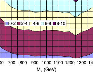
Figure 1: LHC detection prospects for $100\,{\rm fb}^{-1}$ of integrated luminosity in the $\eta$-$M_{X}$ plane. The countours are of signal significance, which exceeds $5$ only when $\eta\lower 3.01385pt\hbox{$\;\stackrel{{\scriptstyle\textstyle>}}{{\sim}}\;$}0.03$.

Detection at the LHC requires $N_{X}/\sqrt{N_{bgd}}>5$ in a single bin normalized to a smooth SM background distribution. We see that realistic demands for a signal which can be distinguished from the background will require $\eta>0.03$. Below the top threshold, the bounds on $\eta$ may shift by $<8\%$. Although this is unfortunately not a good probe when compared to naive one-loop perturbative estimates, the multiplicity of kinetic messengers may enable $\eta>0.03$ and so should be studied with care at the LHC.

The analysis at Tevatron is similar, but with different parameters (accounting for differences in specifications and for a $p\bar{p}$ collider). We now have $C_{ud}=25$ and $\sqrt{s}=2\,{\rm TeV}$. Assuming an integrated luminosity of $8\,{\rm fb}^{-1}$, the $\eta$ sensitivity is

$$\eta_{teva.}\geq\sqrt{N_{X}}e^{-6.7+{m_{X}\over 0.2\,{\rm TeV}}}$$

For detection we demand at least a 5$\sigma$ signal above background, or at least 10 events above background (whichever is larger). At $m_{X}=500\,{\rm GeV}$ detection could only occur if $\eta>0.07$ for this high luminosity. As $m_{X}$ increases, the sensitivity limits on $\eta$ degrade rapidly.

V ILC Prospects

Given the challenge for LHC detection posed by small kinetic mixing, one might hope that ILC can do better. An $e^{+}e^{-}$ collider will generally trade away $\sqrt{s}$ for higher luminosity ($\sim 500\,{\rm fb}^{-1}$) and a cleaner signal. One does not produce an $X$ on resonance, of course, unless its mass is less than the center of mass energy, which we assume here to be $500\,{\rm GeV}$.

The basic process we are interested in is $e^{-}e^{+}\rightarrow\mu\bar{\mu}$ through $\gamma^{*}/Z^{*}/X^{*}$. The observable that provides perhaps the most useful signal in this case is the total cross-sectionLeike:1993ky (the forward-backward asymmetry and left-right polarization do not appear to provide qualitative improvement). We may write the total cross-section as

$$\sigma_{\rm tot}(f\bar{f}) = \frac{N_{c}}{48\pi s}\sum_{n,m}\frac{g^{2}_{n}g^{*2}_{m}s^{2}I^{f}_{m,n}}{(s-m^{2}_{V_{n}})(s-m^{2}_{V_{m}})^{*}}$$ (13)

where

$$I^{f}_{m,n} = (L^{e}_{n}L^{e*}_{m}+R^{e}_{n}R^{e*}_{m})(L^{f}_{n}L^{f*}_{m}+R^{f}_{n}R^{f*}_{m})$$ (14)

and the coupling of the $V_{n}$ boson to the fermions $f\bar{f}$ is given by $ig_{n}\gamma^{\mu}(L^{f}_{n}P_{L}+R^{f}_{n}P_{R})$. If $m_{X}>500\,{\rm GeV}$, this observable will provide the dominant signal. Near the resonance, the signal is enhanced and we should replace:

$$\frac{1}{s-m^{2}_{V}}\Longrightarrow\frac{(s-m^{2}_{V})-i\Gamma_{V}\sqrt{s}}{(s-m^{2}_{V})^{2}+s\,\Gamma_{V}^{2}}\Longrightarrow\frac{-i}{\Gamma_{V}m_{V}}.$$ (15)

Our strategy is to compare the inclusive cross-section for $X$ production to the pure Standard Model background. Our criterion for a signal detection is at least 1% deviation from SM expectations, in order not to run afoul of systematic uncertainties. Recall, we are assuming $500\,{\rm fb}^{-1}$ of integrated luminosity, and so the corresponding statistical significance of the signal is $\sim{\cal L}\sigma_{S}/\sqrt{{\cal L}\sigma_{B}}=0.01\sqrt{{\cal L}\sigma_{B}}\simeq 4.7\sim 5\sigma$, given the SM cross-section $\sigma_{tot}=447$fb COMPHEP . Fig. 2 shows the deviations of $e^{+}e^{-}\rightarrow\mu\bar{\mu}$ at ILC at $\sqrt{s}=500\,{\rm GeV}$ for $500\,{\rm fb}^{-1}$ integrated luminosity. Increasing values of $M_{X}$ can be probed only by increasing values of the mixing parameter $\eta$. For example, $M_{X}=750\,{\rm GeV}$ ($1000\,{\rm GeV}$) can be probed for values of $\eta$ as low as $0.10$ ($0.15$).

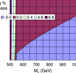
Figure 2: Deviations of $e^{+}e^{-}\rightarrow\mu\bar{\mu}$ at ILC at $\sqrt{s}=500\,{\rm GeV}$ for $500\,{\rm fb}^{-1}$ integrated luminosity are represented in this plot as contours of the $\log_{10}(\%)$ of the excess of events produced compared to SM expectations. The line along the interface of the blue and maroon regions represents a $10^{0}=1\%$ (or $\sim 5\sigma$) deviation.

If $m_{X}<500\,{\rm GeV}$, then we should instead consider the hard-scattering process $e^{-}e^{+}\rightarrow\gamma X\rightarrow\gamma f\bar{f}$. The emission of a hard photon will allow us to scatter through a resonance of the $X$, enhancing the cross-section and yielding a cleaner signal. This is a leading order calculation, as radiation of more photons would serve to enhance both the signal and backgrounds we calculate for the single photon case.

The differential cross-section of $\gamma X$ production is

$${d\sigma\over dx} = {\alpha(c_{L}^{2}+c_{R}^{2})[(s+m_{X}^{2})^{2}+(s-m_{X}^{2})^{2}x^{2}]\over 4s^{2}(s-m_{X}^{2})(1-x^{2})}$$ (16)

where $x\equiv\cos\theta$ and $i\gamma^{\mu}(c_{L}P_{L}+c_{R}P_{R})$ are the couplings of the left and right handed electrons to $X_{\mu}$. We choose a standard $|\cos\theta|<0.95$ angular cut. The signal we analyze signal comment is $X\rightarrow\mu\bar{\mu}$, so we must multiply by the appropriate branching fraction, $B(\mu\bar{\mu})=0.12$. Substituting in the couplings we find

$$\sigma(\gamma X) = \eta^{2}\,\frac{1.26\times 10^{-3}}{s^{2}(s-m_{X}^{2})}F(s,m_{X},x_{0}),~{}~{}{\rm where}$$

$$F(s,m_{X},x_{0}) = (s^{2}+m_{X}^{4})\tanh^{-1}x_{0}-{x_{0}\over 2}(s-m_{X}^{2})^{2}$$

and $x_{0}=|\cos\theta_{min}|=0.95$. Comparing this signal to the Standard Model background $e^{+}e^{-}\rightarrow\gamma\mu\bar{\mu}$ gives us signal significance at ILC for $m_{X}<500\,{\rm GeV}$ as well(Fig.3). We find that kinetimatically accessible $X$ bosons at ILC can be probed and studied perhaps better than at the LHC. Having the ILC data, along with the LHC data, can significantly help us understand all the properties of an exotic massive weakly coupled vector boson Freitas:2004hq .

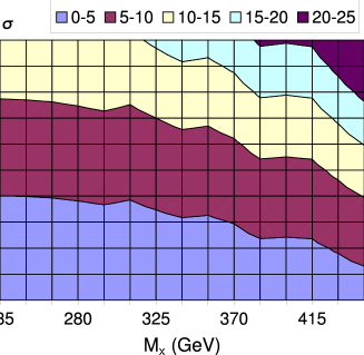
Figure 3: Signal significance plot of $e^{+}e^{-}\rightarrow\gamma X\rightarrow\gamma\mu\bar{\mu}$ at ILC $\sqrt{s}=500\,{\rm GeV}$ with $500\,{\rm fb}^{-1}$ integrated luminosity. We assume that the $m_{\mu\bar{\mu}}$ can be measured to within 2%.

An analysis of LEP data proceeds in a similar manner. For $m_{X}>\sqrt{s}$, detection from LEP data is highly disfavored. For smaller $m_{X}$, however, resonance production (through hard photon emission) is allowed, which favors detection at LEP over hadron colliders such as LHC or the Tevatron. (We assume $725\,{\rm pb}^{-1}$ at $\sqrt{s}=206\,{\rm GeV}$.) But even at these low $m_{X}$ values ILC would provide better detection sensitivity.

VI Outlook

We can summarize our results with a detection plot (Fig.4). We see that for $m_{X}\lower 3.01385pt\hbox{$\;\stackrel{{\scriptstyle\textstyle>}}{{\sim}}\;$}550\,{\rm GeV}$, LHC is more capable of detecting $X_{\mu}$ in our scenario, while for $m_{X}\lower 3.01385pt\hbox{$\;\stackrel{{\scriptstyle\textstyle<}}{{\sim}}\;$}550\,{\rm GeV}$ ILC-500 is more sensitive. Detection within the regime favored by a naive perturbative estimate of kinetic mixing ($\eta\sim 10^{-3}-10^{-2}$) appears difficult at the LHC, but perhaps possible at the ILC as long as the gauge boson mass is at or below the center of mass energy of the ILC. Of course, a higher energy ILC (1 TeV and higher) will help the search for higher-mass $X$ bosons. As we emphasized earlier, however, the amount of kinetic mixing can vary dramatically from one model to the next, depending on the multiplicity of the kinetic messengers, and thus all regions of phase space are candidates for discovery.

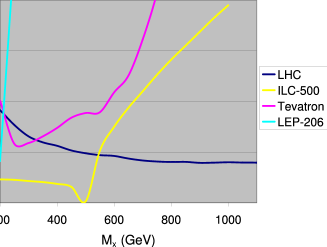
Figure 4: Detection plot of estimated $5\sigma$ confidence level of $X$-boson that kinetically mixes with hypercharge. Detection for Tevatron ($8\,{\rm fb}^{-1}$), LHC ($100\,{\rm fb}^{-1}$), LEP ($\sqrt{s}=206\,{\rm GeV}$ and $725\,{\rm pb}^{-1}$), and ILC ($\sqrt{s}=500\,{\rm GeV}$ and $500\,{\rm fb}^{-1}$) can occur at points above their respective lines.

Acknowledgments. We gratefully acknowledge S.Abel, B.Dutta, B.Holdom, P.Langacker, D.Morrissey, A.Rajaraman, T.Rizzo, G.Shiu and M.Toharia for helpful discussions. This work is supported by the Department of Energy, NSF Grant PHY-0314712 and the MCTP.

References

- (1) J. L. Hewett and T. G. Rizzo, Phys. Rept. 183, 193 (1989).
- (2) M. Cvetic and P. Langacker, Phys. Rev. D 54, 3570 (1996) [hep-ph/9511378].
- (3) A. Leike, Phys. Lett. B 402, 374 (1997) [hep-ph/9703263].
- (4) J. Kang and P. Langacker, Phys. Rev. D 71, 035014 (2005) [hep-ph/0412190].
- (5) J. Kumar, Int. J. Mod. Phys. A 21, 3441 (2006) [arXiv:hep-th/0601053].
- (6) M. R. Douglas and S. Kachru, arXiv:hep-th/0610102.
- (7) G. Aldazabal et al., JHEP 0102, 047 (2001) [hep-ph/0011132].
- (8) R. Blumenhagen, M. Cvetic, P. Langacker and G. Shiu, hep-th/0502005.
- (9) F. Marchesano and G. Shiu, JHEP 0411, 041 (2004) [hep-th/0409132].
- (10) J. Kumar and J. D. Wells, Phys. Rev. D 71, 026009 (2005) [hep-th/0409218]; JHEP 0509, 067 (2005) [hep-th/0506252]; hep-th/0604203.
- (11) T. P. T. Dijkstra, L. R. Huiszoon and A. N. Schellekens, Nucl. Phys. B 710, 3 (2005) [hep-th/0411129].
- (12) F. Gmeiner et al., JHEP 0601, 004 (2006) [hep-th/0510170].
- (13) K. R. Dienes, C. F. Kolda and J. March-Russell, Nucl. Phys. B 492, 104 (1997) [hep-ph/9610479].
- (14) S. P. Martin, Phys. Rev. D 54, 2340 (1996) [hep-ph/9602349].
- (15) T. G. Rizzo, Phys. Rev. D 59, 015020 (1999) [hep-ph/9806397].
- (16) F. del Aguila, M. Masip and M. Perez-Victoria, Nucl. Phys. B 456, 531 (1995) [hep-ph/9507455].
- (17) B. Holdom, Phys. Lett. B 166, 196 (1986).
- (18) B. A. Dobrescu, Phys. Rev. Lett. 94, 151802 (2005) [hep-ph/0411004].
- (19) K. S. Babu, C. F. Kolda and J. March-Russell, Phys. Lett. B 408, 261 (1997) [hep-ph/9705414].
- (20) S. A. Abel and B. W. Schofield, Nucl. Phys. B 685, 150 (2004) [hep-th/0311051].
- (21) T. Appelquist, B. A. Dobrescu and A. R. Hopper, Phys. Rev. D 68, 035012 (2003) [arXiv:hep-ph/0212073].
- (22) M. E. Peskin and T. Takeuchi, Phys. Rev. D 46, 381 (1992).
- (23) B. Holdom, Phys. Lett. B 259, 329 (1991).
- (24) LEP Electroweak Working Group, “A combination of preliminary electroweak measurements and constraints on the standard model,” arXiv:hep-ex/0511027.
- (25) W. M. Yao et al. [Particle Data Group], J. Phys. G 33, 1 (2006).
- (26) See for example, ATLAS TDR, CERN/LHCC/94-43 (15 December 1994).
- (27) M. Dittmar, A. S. Nicollerat and A. Djouadi, Phys. Lett. B 583, 111 (2004) [arXiv:hep-ph/0307020].
- (28) T. Sjostrand, S. Mrenna and P. Skands, hep-ph/0603175.
- (29) A. Leike, Z. Phys. C 62, 265 (1994) [hep-ph/9311356].
- (30) A. Pukhov et al. (COMPHEP), hep-ph/9908288.
- (31) We choose as a specific final state, but detection of the boson can come from any decay channel (including invisible) by looking for the peak in photon-recoil spectrum. Definitive final states, such as invariant mass peak however are sharp signals of the -boson mass and branching fraction into .
- (32) A. Freitas, Phys. Rev. D 70, 015008 (2004) [arXiv:hep-ph/0403288].