Abstract

We present the first quenched lattice QCD study of the form factors relevant for the hyperon semileptonic decay $\Sigma^{-}\rightarrow n~{}\ell~{}\nu$. The momentum dependence of both axial and vector form factors is investigated and the values of all the form factors at zero-momentum transfer are presented. Following the same strategy already applied to the decay $K^{0}\rightarrow\pi^{-}\ell~{}\nu$, the SU(3)-breaking corrections to the vector form factor at zero-momentum transfer, $f_{1}(0)$, are determined with great statistical accuracy in the regime of the simulated quark masses, which correspond to pion masses above $\approx 0.7$ GeV. Besides $f_{1}(0)$ also the axial to vector ratio $g_{1}(0)/f_{1}(0)$, which is relevant for the extraction of the CKM matrix element $V_{us}$, is determined with significant accuracy. Due to the heavy masses involved, a polynomial extrapolation, which does not include the effects of meson loops, is performed down to the physical quark masses, obtaining $f_{1}(0)=-0.948\pm 0.029$ and $g_{1}(0)/f_{1}(0)=-0.287\pm 0.052$, where the uncertainties do not include the quenching effect. Adding a recent next-to-leading order determination of chiral loops, calculated within the Heavy Baryon Chiral Perturbation Theory in the approximation of neglecting the decuplet contribution, we obtain $f_{1}(0)=-0.988\pm 0.029_{\rm lattice}\pm 0.040_{\rm HBChPT}$. Our findings indicate that SU(3)-breaking corrections are moderate on both $f_{1}(0)$ and $g_{1}(0)$. They also favor the experimental scenario in which the weak electricity form factor, $g_{2}(0)$, is large and positive, and correspondingly the value of $|g_{1}(0)/f_{1}(0)|$ is reduced with respect to the one obtained with the conventional assumption $g_{2}(q^{2})=0$ based on exact SU(3) symmetry.

1 Introduction

Recently it has been shown that SU(3)-breaking corrections to the $K\to\pi$ vector form factor can be determined from lattice simulations with great precision [1]. The approach has allowed to reach the percent level of accuracy in the extraction of $V_{us}$ from $K_{\ell 3}$ decays, thus stimulating new unquenched lattice studies to reduce the systematic uncertainty [2]. An independent way to extract $V_{us}$ is provided by hyperon semileptonic decays, and Ref. [3] has shown that it is possible to extract the product $|V_{us}\cdot f_{1}(0)|$ at the percent level from hyperon experiments, where $f_{1}(0)$ is the vector form factor (f.f.) at zero-momentum transfer. The Ademollo-Gatto (AG) theorem [4] protects $f_{1}(0)$ from first-order SU(3)-breaking corrections that are thus suppressed. Experiments seem to be consistent with negligible channel-dependent SU(3) corrections in this f.f. [3], but they cannot exclude sizable (i.e. larger than percent), channel-independent effects in the extraction of $V_{us}$. Model dependent estimates based on quark models, $1/N_{c}$ and chiral expansions give different results (see e.g. Ref. [5]), so that a lattice QCD determination of $f_{1}(0)$, as well as of all the other vector and axial f.f.’s which are not AG protected, is of great interest.

The aim of the present work is to investigate SU(3)-breaking corrections to both vector and axial form factors relevant for the $\Sigma^{-}\rightarrow n$ transition, completing and generalizing in this way the preliminary lattice study of Ref. [6]. Though our simulation is carried out in the quenched approximation, our results represent the first attempt to evaluate hyperon f.f.’s using a non-perturbative method based only on QCD.

We first show that it is possible to determine the SU(3)-breaking corrections to $f_{1}(0)$ on the lattice following the method of Ref. [1], which is based on the following three main steps: i) evaluation of the scalar form factor $f_{0}(q^{2})$ at $q^{2}=q_{\rm max}^{2}=(M_{\Sigma}-M_{n})^{2}$; ii) study of the momentum dependence of $f_{0}(q^{2})$ to extrapolate $f_{0}(q_{\rm max}^{2})$ down to $f_{0}(0)=f_{1}(0)$; and iii) extrapolation in the quark masses down to the physical point. The latter step is one of the main sources of uncertainty in the quenched lattice calculations of the vector f.f., since the AG theorem makes this quantity dominated by meson loops. We make use of the recent, next-to-leading order (NLO) calculation of the chiral corrections to $f_{1}(0)$ performed in Ref. [7] within the Heavy Baryon Chiral Perturbation Theory (HBChPT). As in the meson sector, the AG theorem prevents the contribution from local counter-terms up to $O(p^{4})$ and makes the NLO corrections finite and free from unknown low-energy parameters. However, the convergence of the chiral expansion turns out to be rather poor and the inclusion of the decuplet contribution appears to spoil the expansion itself [7]. Thus, the third step of the procedure of Ref. [1], i.e. the correction of the leading quenched chiral logs with the full QCD ones, is not possible in the hyperon case. In this respect we note that the use of HBChPT in conjunction with lattice QCD is likely to represent a serious limitation for achieving a precise determination of $f_{1}(0)$ also in future (unquenched) lattice calculations, until it will be possible to simulate on the lattice very light quark masses, close to the physical ones, and sufficiently large volumes [8].

Due to the rather heavy masses involved in our simulation, it is unlikely that meson loops can contribute significantly at the simulated quark masses. Thus a polynomial extrapolation, which does not include the effects of meson loops, is performed down to the physical quark masses, leading to $f_{1}(0)=-0.948\pm 0.029$. This result for the SU(3)-breaking corrections, corresponding to $f_{1}(0)+1=(5.2\pm 2.9)\%$, represents mainly an estimate of the local terms of the chiral expansion and appears to be opposite in both sign and size to the NLO estimate of chiral loops, $(-4\pm 4)\%$, calculated in Ref. [7] in the approximation of neglecting the decuplet contribution and assuming a $100\%$ overall uncertainty. The two contributions should be added, leading to our final estimate: $f_{1}(0)=-0.988\pm 0.029_{\rm lattice}\pm 0.040_{\rm HBChPT}$, where the uncertainties do not include the quenching effect.

Second, we investigate the momentum dependence of the other two vector f.f.’s, the weak magnetism $f_{2}(q^{2})$ and the induced scalar $f_{3}(q^{2})$, as well as of the three axial f.f.’s, the axial-vector $g_{1}(q^{2})$, the weak electricity $g_{2}(q^{2})$ and the induced pseudoscalar $g_{3}(q^{2})$.

The ratio $g_{1}(q^{2})/f_{1}(q^{2})$ can be determined with quite good statistical accuracy directly from the ratio of appropriate axial and vector three-point correlation functions. We show that such a ratio can be evaluated on the lattice at $q^{2}=q_{\rm max}^{2}$ (i.e. with hyperons at rest) within $\approx 10\%$ accuracy and that the extrapolation down to $q^{2}=0$ does not modify significantly that level of precision. Adopting a polynomial extrapolation in the quark masses we get $g_{1}(0)/f_{1}(0)=-0.287\pm 0.052$, which is consistent with the value $g_{1}(0)/f_{1}(0)=-0.340\pm 0.017$ adopted in the recent analysis of Ref. [3]. The study of the degenerate transitions also allows to determine the value of $g_{1}(0)/f_{1}(0)$ directly in the SU(3) limit; we get $[g_{1}(0)/f_{1}(0)]_{SU(3)}=-0.269\pm 0.047$. Compared with the above estimate, it implies that the SU(3)-breaking corrections on $g_{1}(0)/f_{1}(0)$ are moderate, though this ratio is not protected by the AG theorem. Our finding is in qualitative agreement with the exact SU(3)-symmetry assumption of the Cabibbo model [9].

Contrary to $f_{1}(q^{2})$ and $g_{1}(q^{2})$, the other f.f.’s cannot be evaluated at $q^{2}=q_{\rm max}^{2}$ and consequently the extrapolation of the lattice data to $q^{2}=0$ is affected by larger uncertainties. In the cases of the weak magnetism and of the induced pseudoscalar f.f.’s, whose matrix elements do not vanish in the SU(3) limit, we obtain $f_{2}(0)/f_{1}(0)=-1.52\pm 0.81$ and $g_{3}(0)/f_{1}(0)=6.1\pm 3.3$ at the physical point. The central values agree well with the experimental result $f_{2}(0)/f_{1}(0)=-1.71\pm 0.12_{\rm stat.}\pm 0.23_{\rm syst.}$ from Ref. [10], as well as with the SU(3)-breaking analysis of Ref. [11], and with the value $g_{3}(0)/f_{1}(0)=5.5\pm 0.9$, obtained using the axial Ward Identity and the generalized Goldberger-Treiman relation [12], which relates $g_{3}(0)$ with $g_{1}(0)$ in the chiral limit.

For the weak electricity $g_{2}(q^{2})$ and the induced scalar $f_{3}(q^{2})$ f.f.’s a non-vanishing result, which is entirely due to SU(3)-breaking corrections, is found, namely $g_{2}(0)/f_{1}(0)=0.63\pm 0.26$ and $f_{3}(0)/f_{1}(0)=-0.42\pm 0.22$. Note that experiments carried out with polarized $\Sigma^{-}$ hyperons [10] have determined the f.f. combination $|g_{1}(0)/f_{1}(0)-0.133~{}g_{2}(0)/f_{1}(0)|$ to be equal to $0.327\pm 0.007_{\rm stat.}\pm 0.019_{\rm syst.}$. Our result is $0.37\pm 0.08$, which means that the lattice results for both $g_{1}(0)/f_{1}(0)$ and $g_{2}(0)/f_{1}(0)$ are nicely consistent with the experimental data on the $\Sigma^{-}\rightarrow n$ transition. Our findings favor the scenario in which $g_{2}(0)/f_{1}(0)$ is large and positive, and correspondingly the value of $|g_{1}(0)/f_{1}(0)|$ is reduced with respect to the one obtained with the conventional assumption $g_{2}(q^{2})=0$ (done in Ref. [3]) based on exact SU(3) symmetry. Such a scenario is slightly preferred also by experimental data (see Ref. [10]).

The plan of the paper is as follows. In Section 2 we introduce the notation and give some details about the lattice simulation. Section 3 is devoted to the extraction of $f_{0}(q^{2})$ at $q^{2}=q_{\rm max}^{2}$, to its extrapolation down to $q^{2}=0$ and to the polynomial extrapolation in the quark masses down to their physical values, without taking into account the effects of meson loops. The estimate of these effects, based on HBChPT at the NLO, is described in Section 4, where the problematic related to the convergence of the chiral expansion and to the decuplet contribution is briefly illustrated. In Section 5 we present our results for the ratio $g_{1}(0)/f_{1}(0)$, while those for the other vector and axial f.f.’s are collected in Section 6. Finally our conclusions are given in Section 7.

2 Notation and Lattice Details

In this study we restrict our attention to the $\Sigma^{-}\rightarrow n~{}l~{}\nu$ decay. We are interested in the hadronic matrix element of the weak ($V-A$) current, $\mathcal{M}\equiv\langle n|\overline{u}\gamma_{\mu}(1-\gamma_{5})s|\Sigma^{-}\rangle$, which can be conveniently expressed in Minkowski space in terms of f.f.’s and external spinors as

$$\mathcal{M} = \overline{u}_{n}(p^{\prime})\left\{\gamma^{\mu}f_{1}(q^{2})-i\frac{\sigma^{\mu\nu}q_{\nu}}{M_{n}+M_{\Sigma}}f_{2}(q^{2})+\frac{q^{\mu}}{M_{n}+M_{\Sigma}}f_{3}(q^{2})\right.$$ (1)

$$+ \left[\left.\gamma^{\mu}g_{1}(q^{2})-i\frac{\sigma^{\mu\nu}q_{\nu}}{M_{n}+M_{\Sigma}}g_{2}(q^{2})+\frac{q^{\mu}}{M_{n}+M_{\Sigma}}g_{3}(q^{2})\right]\gamma_{5}\right\}u_{\Sigma}(p)$$

$$= \overline{u}_{n}(p^{\prime})\left\{O^{\mu}_{V}+O^{\mu}_{A}\right\}u_{\Sigma}(p)~{}~{}~{}~{}~{}~{}$$

with $q=p-p^{\prime}$. A detailed discussion of the properties of the six f.f.’s in Eq. (1) can be found, e.g., in Ref. [3]. We also introduce the scalar f.f. $f_{0}(q^{2})$ from the divergence of the vector weak current $\langle n|\partial_{\mu}~{}V^{\mu}|\Sigma^{-}\rangle\equiv(M_{\Sigma}+M_{n})f_{0}(q^{2})$. It is related to $f_{1}(q^{2})$ and $f_{3}(q^{2})$ by

$$f_{0}(q^{2})=f_{1}(q^{2})+\frac{q^{2}}{M_{\Sigma}^{2}-M_{n}^{2}}~{}f_{3}(q^{2})~{},$$ (2)

and at $q^{2}=0$ it coincides with the quantity of interest $f_{1}(0)$. Note that for the $\Sigma^{-}\rightarrow n$ transition $f_{1}(0)$ is normalized as $f_{1}(0)=-1$ in the SU(3) limit.

In order to access the matrix element of Eq. (1) on the lattice, one can consider the following two- and three-point correlation functions in euclidean space

$$\left[G^{\Sigma(n)}(t,\vec{p})\right]_{\gamma^{\prime}\gamma} = \sum_{\vec{x}}\langle J^{\Sigma(n)}_{\gamma^{\prime}}(t,\vec{x})\bar{J}^{\Sigma(n)}_{\gamma}(0,\vec{0})\rangle e^{-i\vec{p}\cdot\vec{x}}~{},$$ (3)

$$\left[V^{\Sigma n}_{\mu}(t_{x},t_{y},\vec{p},\vec{p}\,^{\prime})\right]_{\gamma^{\prime}\gamma} = \langle J_{\gamma^{\prime}}^{n}(t_{y},\vec{y})\widehat{V}_{\mu}(t_{x},\vec{x})\bar{J}_{\gamma}^{\Sigma}(0,\vec{0})\rangle e^{-i(\vec{p}-\vec{p}\,^{\prime})\cdot\vec{x}}~{}e^{-i\vec{p}\,^{\prime}\cdot\vec{y}}~{},$$ (4)

$$\left[A^{\Sigma n}_{\mu}(t_{x},t_{y},\vec{p},\vec{p}\,^{\prime})\right]_{\gamma^{\prime}\gamma} = \langle J_{\gamma^{\prime}}^{n}(t_{y},\vec{y})\widehat{A}_{\mu}(t_{x},\vec{x})\bar{J}_{\gamma}^{\Sigma}(0,\vec{0})\rangle e^{-i(\vec{p}-\vec{p}\,^{\prime})\cdot\vec{x}}~{}e^{-i\vec{p}\,^{\prime}\cdot\vec{y}}~{},~{}~{}~{}~{}~{}$$ (5)

where $J^{n,\Sigma}_{\gamma}$ are local interpolating operators for the neutron and the $\Sigma^{-}$ hyperon, which we choose to be

$$J^{n}_{\alpha}=\varepsilon_{ijk}[d^{T}_{i}C\gamma_{5}u_{j}]d_{k\alpha}~{},\quad J^{\Sigma}_{\alpha}=\varepsilon_{ijk}[d^{T}_{i}C\gamma_{5}s_{j}]d_{k\alpha}~{},$$ (6)

with latin (greek) symbols referring to color (Dirac) indices. The operators in Eq. (6) are related to the external spinors $u_{\Sigma,n}$ (cf. Eq. (1)) via the relation

$$\langle 0|J_{\gamma}^{\Sigma(n)}(\vec{0},0)|{\Sigma(n)}(\vec{p},\sigma)\rangle=\sqrt{Z_{\Sigma(n)}}\left[u_{\Sigma(n)}(p,\sigma)\right]_{\gamma}~{},$$ (7)

where $\sigma$ refers to the polarization of the $\Sigma(n)$ baryon.

In Eqs. (4)-(5) $\widehat{V}_{\mu}$ and $\widehat{A}_{\mu}$ are the renormalized, $O(a)$-improved lattice weak vector and axial-vector current respectively:

$$\widehat{V}^{\mu} = Z_{V}\left(1+b_{V}\frac{am_{s}+am_{\ell}}{2}\right)\left(\bar{u}\gamma^{\mu}s~{}+~{}ac_{V}\partial_{\nu}~{}\bar{u}\sigma^{\mu\nu}s\right)~{},$$ (8)

$$\widehat{A}^{\mu} = Z_{A}\left(1+b_{A}\frac{am_{s}+am_{\ell}}{2}\right)\left(\bar{u}\gamma^{\mu}\gamma_{5}s~{}+~{}ac_{A}\partial^{\mu}~{}\bar{u}\gamma_{5}s\right)\,,$$ (9)

where $Z_{V}$ and $Z_{A}$ are the vector and axial-vector renormalization constants, $b_{V}$, $b_{A}$, $c_{V}$ and $c_{A}$ are $O(a)$-improvement coefficients [13] and the subscript $\ell$ refers to the light $u$ or $d$ quarks, which we consider to be degenerate in mass.

Taking the large-time limits $t_{x},(t_{y}-t_{x})\to\infty$ and using (7) one can rewrite Eqs. (3)-(4) as follows

$$\left[G^{\Sigma(n)}(t,\vec{p}(\vec{p}\,^{\prime}))\right]_{\gamma^{\prime}\gamma} {}_{\overrightarrow{\mbox{\tiny$t\to\infty$}}}~{}Z_{\Sigma(n)}e^{-E_{\Sigma(n)}t}\left(\frac{ip{\hskip-4.83694pt}/(p{\hskip-4.83694pt}/\,^{\prime})+M_{\Sigma(n)}}{2E_{\Sigma(n)}}\right)_{\gamma^{\prime}\gamma}~{},$$ (12)

$$\left[V_{\mu}^{\Sigma n}(t_{x},t_{y},\vec{p},\vec{p}\,^{\prime})\right]_{\gamma^{\prime}\gamma} ~{}_{\overrightarrow{\mbox{\tiny$t_{x},(t_{y}-t_{x})\to\infty$}}}~{}e^{-E_{n}t_{x}}e^{-E_{\Sigma}(t_{y}-t_{x})}\sqrt{Z_{n}Z_{\Sigma}}\cdot$$

$$\hskip 71.13188pt\left(\frac{ip{\hskip-4.83694pt}/\,^{\prime}+M_{n}}{2E_{n}}\right)_{\gamma^{\prime}\rho}(O_{\mu}^{V})_{\rho\sigma}\left(\frac{ip{\hskip-4.83694pt}/+M_{\Sigma}}{2E_{\Sigma}}\right)_{\sigma\gamma}~{},$$

$$\left[A_{\mu}^{\Sigma n}(t_{x},t_{y},\vec{p},\vec{p}\,^{\prime})\right]_{\gamma^{\prime}\gamma} ~{}_{\overrightarrow{\mbox{\tiny$t_{x},(t_{y}-t_{x})\to\infty$}}}~{}e^{-E_{n}t_{x}}e^{-E_{\Sigma}(t_{y}-t_{x})}\sqrt{Z_{n}Z_{\Sigma}}\cdot$$

$$\hskip 71.13188pt\left(\frac{ip{\hskip-4.83694pt}/\,^{\prime}+M_{n}}{2E_{n}}\right)_{\gamma^{\prime}\rho}(O_{\mu}^{A})_{\rho\sigma}\left(\frac{ip{\hskip-4.83694pt}/+M_{\Sigma}}{2E_{\Sigma}}\right)_{\sigma\gamma}~{},~{}~{}~{}~{}~{}$$

where $E_{n}=\sqrt{M_{n}^{2}+|\vec{p}\,^{\prime}|^{2}}$, $E_{\Sigma}=\sqrt{M_{\Sigma}^{2}+|\vec{p}|^{2}}$ and $O_{\mu}^{V}$ ($O_{\mu}^{A}$) is the euclidean version of the vector (axial-vector) contribution to Eq. (1). From Eqs. (12) and (12) it follows

$$\frac{V_{\mu}^{\Sigma n}(t_{x},t_{y},\vec{p},\vec{p}\,^{\prime})_{\gamma^{\prime}\gamma}}{G^{\Sigma}(t_{x},\vec{p})_{\gamma^{\prime}\gamma}G^{n}(t_{y}-t_{x},\vec{p}\,^{\prime})}_{\gamma^{\prime}\gamma}\phantom{.}{}_{\overrightarrow{\mbox{\tiny$t_{x},(t_{y}-t_{x})\to\infty$}}}\frac{1}{\sqrt{Z_{n}Z_{\Sigma}}}\frac{[(ip{\hskip-4.83694pt}/\,^{\prime}+M_{n})O_{\mu}^{V}(ip{\hskip-4.83694pt}/+M_{\Sigma})]_{\gamma^{\prime}\gamma}}{(ip{\hskip-4.83694pt}/\,^{\prime}+M_{n})_{\gamma^{\prime}\gamma}~{}(ip{\hskip-4.83694pt}/+M_{\Sigma})_{\gamma^{\prime}\gamma}}~{},$$ (13)

$$\frac{A_{\mu}^{\Sigma n}(t_{x},t_{y},\vec{p},\vec{p}\,^{\prime})_{\gamma^{\prime}\gamma}}{G^{\Sigma}(t_{x},\vec{p})_{\gamma^{\prime}\gamma}G^{n}(t_{y}-t_{x},\vec{p}\,^{\prime})}_{\gamma^{\prime}\gamma}\phantom{.}{}_{\overrightarrow{\mbox{\tiny$t_{x},(t_{y}-t_{x})\to\infty$}}}\frac{1}{\sqrt{Z_{n}Z_{\Sigma}}}\frac{[(ip{\hskip-4.83694pt}/\,^{\prime}+M_{n})O_{\mu}^{A}(ip{\hskip-4.83694pt}/+M_{\Sigma})]_{\gamma^{\prime}\gamma}}{(ip{\hskip-4.83694pt}/\,^{\prime}+M_{n})_{\gamma^{\prime}\gamma}~{}(ip{\hskip-4.83694pt}/+M_{\Sigma})_{\gamma^{\prime}\gamma}}~{}.$$ (14)

Let us consider the following kinematics

$$p=(\sqrt{M^{2}_{\Sigma}+|\vec{q}|^{2}},\vec{q})\equiv(E_{q},\vec{q}),~{}~{}~{}~{}p^{\prime}=(M_{n},\vec{0})$$ (15)

and study the matrix elements of the weak vector current. In order to minimize the number of calculated three-point correlation functions we consider only one pair of values of the Dirac indices, namely $\gamma=\gamma^{\prime}=0$. Then we define the following quantities

$$W_{1}(q^{2};t_{x},t_{y}) \equiv \frac{2E_{q}\sqrt{Z_{n}Z_{\Sigma}}}{E_{q}+M_{\Sigma}}\frac{{\rm Re}\left(V^{\Sigma n}_{0}(t_{x},t_{y},\vec{q},\vec{0})_{00}\right)}{G^{\Sigma}(t_{x},\vec{q})_{00}~{}G^{n}(t_{y}-t_{x},\vec{0})_{00}}~{},$$

$$W_{2}(q^{2};t_{x},t_{y}) \equiv \frac{2E_{q}\sqrt{Z_{n}Z_{\Sigma}}}{|\vec{q}|^{2}}\frac{{\rm Im}\left(q_{k}V^{\Sigma n}_{k}(t_{x},t_{y},\vec{q},\vec{0})_{00}\right)}{G^{\Sigma}(t_{x},\vec{q})_{00}~{}G^{n}(t_{y}-t_{x},\vec{0})_{00}}~{},$$

$$W_{3}(q^{2};t_{x},t_{y}) \equiv \frac{2E_{q}\sqrt{Z_{n}Z_{\Sigma}}}{q_{1}}\frac{{\rm Re}\left(V^{\Sigma n}_{2}(t_{x},t_{y},\vec{q},\vec{0})_{00}\right)}{G^{\Sigma}(t_{x},\vec{q})_{00}~{}G^{n}(t_{y}-t_{x},\vec{0})_{00}}~{},$$ (16)

which in terms of the three vector form factors $f_{1,2,3}$ read as

$$\overline{W}_{1}(q^{2}) = f_{1}(q^{2})-\frac{E_{q}-M_{\Sigma}}{M_{\Sigma}+M_{n}}f_{2}(q^{2})+\frac{E_{q}-M_{n}}{M_{\Sigma}+M_{n}}f_{3}(q^{2})~{},$$

$$\overline{W}_{2}(q^{2}) = f_{1}(q^{2})-\frac{E_{q}-M_{n}}{M_{\Sigma}+M_{n}}f_{2}(q^{2})+\frac{E_{q}+M_{\Sigma}}{M_{\Sigma}+M_{n}}f_{3}(q^{2})~{},$$

$$\overline{W}_{3}(q^{2}) = f_{1}(q^{2})+f_{2}(q^{2})~{},$$ (17)

where $\overline{W}_{i}(q^{2})\equiv\mbox{lim}_{\mbox{\tiny$t_{x},(t_{y}-t_{x})\to\infty$}}~{}W_{i}(q^{2};t_{x},t_{y})$ ($i=1,2,3$). Inverting the above equations one gets

$$f_{1}(q^{2}) = {\cal{N}}\Bigl{\{}\overline{W}_{1}(q^{2})-\frac{E_{q}-M_{n}}{E_{q}+M_{\Sigma}}\overline{W}_{2}(q^{2})-\frac{q^{2}}{(M_{\Sigma}+M_{n})(E_{q}+M_{\Sigma})}\overline{W}_{3}(q^{2})\Bigl{\}},~{}~{}~{}~{}~{}~{}~{}~{}$$ (18)

$$f_{2}(q^{2}) = {\cal{N}}\Bigl{\{}-\overline{W}_{1}(q^{2})+\frac{E_{q}-M_{n}}{E_{q}+M_{\Sigma}}\overline{W}_{2}(q^{2})+\frac{M_{\Sigma}+M_{n}}{E_{q}+M_{\Sigma}}\overline{W}_{3}(q^{2})\Bigl{\}},~{}~{}~{}~{}~{}~{}~{}~{}$$ (19)

$$f_{3}(q^{2}) = {\cal{N}}\Bigl{\{}-\overline{W}_{1}(q^{2})+\frac{E_{q}+M_{n}}{E_{q}+M_{\Sigma}}\overline{W}_{2}(q^{2})+\frac{q^{2}}{(M_{\Sigma}-M_{n})(E_{q}+M_{\Sigma})}\overline{W}_{3}(q^{2})\Bigl{\}}~{}~{}~{}~{}~{}~{}~{}~{}$$ (20)

with ${\cal{N}}\equiv(M_{\Sigma}+M_{n})/2M_{n}$.

Equations (16)-(20) provide the standard procedure for measuring f.f.’s on the lattice. Typically the accuracy that can be reached in this way is not better than $10\div 20\%$, which is clearly not sufficient for measuring SU(3)-breaking effects in $f_{1}(0)$ at the percent level. In the next Section we describe the procedure to get both the scalar form factor (2) at $q^{2}=q_{\rm max}^{2}$ and the ratios $f_{2}(q^{2})/f_{1}(q^{2})$ and $f_{3}(q^{2})/f_{1}(q^{2})$ with quite small statistical fluctuations.

In the case of the axial-vector weak current, choosing always $\gamma=\gamma^{\prime}=0$, we define the following quantities

$$W_{1}^{(A)}(q^{2};t_{x},t_{y}) \equiv \frac{2E_{q}\sqrt{Z_{n}Z_{\Sigma}}}{E_{q}+M_{\Sigma}}\frac{{\rm Im}\left(\tilde{A}^{\Sigma n}(t_{x},t_{y},\vec{q},\vec{0})_{00}\right)}{G^{\Sigma}(t_{x},\vec{q})_{00}~{}G^{n}(t_{y}-t_{x},\vec{0})_{00}}~{},$$

$$W_{2}^{(A)}(q^{2};t_{x},t_{y}) \equiv \frac{2E_{q}\sqrt{Z_{n}Z_{\Sigma}}}{q_{3}}\frac{{\rm Re}\left(A^{\Sigma n}_{0}(t_{x},t_{y},\vec{q},\vec{0})_{00}\right)}{G^{\Sigma}(t_{x},\vec{q})_{00}~{}G^{n}(t_{y}-t_{x},\vec{0})_{00}}~{},$$

$$W_{3}^{(A)}(q^{2};t_{x},t_{y}) \equiv -\frac{2E_{q}(M_{\Sigma}+M_{n})\sqrt{Z_{n}Z_{\Sigma}}}{q_{1}q_{3}}\frac{{\rm Im}\left(A^{\Sigma n}_{1}(t_{x},t_{y},\vec{q},\vec{0})_{00}\right)}{G^{\Sigma}(t_{x},\vec{q})_{00}~{}G^{n}(t_{y}-t_{x},\vec{0})_{00}}~{},~{}~{}~{}~{}$$ (21)

where $\tilde{A}^{\Sigma n}\equiv A^{\Sigma n}_{3}+\left(A^{\Sigma n}_{1}/q_{1}+A^{\Sigma n}_{2}/q_{2}\right)\cdot\left(|\vec{q}|^{2}-q_{3}^{2}\right)/2q_{3}$. In terms of the three axial-vector form factors $g_{1,2,3}$ one has

$$\overline{W}_{1}^{(A)}(q^{2}) = g_{1}(q^{2})-\frac{E_{q}-M_{n}}{M_{\Sigma}+M_{n}}g_{2}(q^{2})+\frac{E_{q}-M_{\Sigma}}{M_{\Sigma}+M_{n}}g_{3}(q^{2})~{},$$

$$\overline{W}_{2}^{(A)}(q^{2}) = g_{1}(q^{2})-\frac{E_{q}+M_{\Sigma}}{M_{\Sigma}+M_{n}}g_{2}(q^{2})+\frac{E_{q}-M_{n}}{M_{\Sigma}+M_{n}}g_{3}(q^{2})~{},$$

$$\overline{W}_{3}^{(A)}(q^{2}) = g_{2}(q^{2})-g_{3}(q^{2})~{},$$ (22)

where $\overline{W}_{i}^{(A)}(q^{2})\equiv\mbox{lim}_{\mbox{\tiny$t_{x},(t_{y}-t_{x})\to\infty$}}~{}W_{i}^{(A)}(q^{2};t_{x},t_{y})$ ($i=1,2,3$). Inverting the above equations one gets

$$g_{1}(q^{2}) = {\cal{N}}\Bigl{\{}\overline{W}_{1}^{(A)}(q^{2})+\frac{M_{n}-M_{\Sigma}}{M_{n}+M_{\Sigma}}\overline{W}_{2}^{(A)}(q^{2})+\frac{1}{(M_{n}+M_{\Sigma})^{2}}\overline{W}_{3}^{(A)}(q^{2})$$ (23)

$$\cdot ~{}~{}~{}~{}\left[(M_{n}-M_{\Sigma})(E_{q}-M_{n})-(M_{n}+M_{\Sigma})(E_{q}-M_{\Sigma})\right]\Bigl{\}},~{}~{}$$

$$g_{2}(q^{2}) = {\cal{N}}\Bigl{\{}\overline{W}_{1}^{(A)}(q^{2})-\overline{W}_{2}^{(A)}(q^{2})+\frac{M_{n}-M_{\Sigma}}{M_{n}+M_{\Sigma}}\overline{W}_{3}^{(A)}(q^{2})\Bigl{\}},~{}~{}$$ (24)

$$g_{3}(q^{2}) = {\cal{N}}\Bigl{\{}\overline{W}_{1}^{(A)}(q^{2})-\overline{W}_{2}^{(A)}(q^{2})-\overline{W}_{3}^{(A)}(q^{2})\Bigl{\}}~{}.$$ (25)

We have generated $240$ quenched gauge field configurations on a $24^{3}\times 56$ lattice at $\beta=6.20$ (corresponding to an inverse lattice spacing equal to $a^{-1}\simeq 2.6$ GeV), with the plaquette gauge action. We have used the non-perturbatively $O(a)$-improved Wilson fermions with $c_{SW}=1.614$ [14] and chosen quark masses corresponding to four values of the hopping parameters, namely $k\in\{0.1336,0.1340,0.1343,0.1345\}$. Using $\Sigma$ and $n$ baryons with quark content ($k_{s}k_{\ell}k_{\ell}$) and ($k_{\ell}k_{\ell}k_{\ell}$) respectively, twelve different $\Sigma\to n$ vector (axial) correlation functions $V_{\mu}^{\Sigma n}$ ($A_{\mu}^{\Sigma n}$) have been computed, using both $k_{s}<k_{\ell}$ and $k_{s}>k_{\ell}$, corresponding to the cases in which the $\Sigma$(neutron) is heavier than the neutron($\Sigma$). In addition, using the same combinations of quark masses, also the three-point $n\to\Sigma$ correlation functions $V_{\mu}^{n\Sigma}$ ($A_{\mu}^{n\Sigma}$) have been calculated. Finally, twelve elastic, non-degenerate $V_{\mu}^{\Sigma\Sigma}$ ($A_{\mu}^{\Sigma\Sigma}$) and four elastic, fully degenerate $V_{\mu}^{nn}$ ($A_{\mu}^{nn}$) three-point functions have been evaluated.

The simulated quark masses are approximately in the range $\approx 1\div 1.5\times m_{s}$, where $m_{s}$ is the strange quark mass, and correspond to pseudoscalar meson masses in the interval $\approx 0.70\div 1$ GeV and to baryon masses in the range $\approx 1.5\div 1.8$ GeV. Though the simulated meson masses are larger than the physical ones, the corresponding values of $q_{\rm max}^{2}=(M_{\Sigma}-M_{n})^{2}$ are taken as close as possible to $q^{2}=0$ (see Table 1 in the next Section).

To improve the statistics, two- and three-point correlation functions have been averaged with respect to parity and charge conjugation transformations. We have chosen $t_{y}/a=24$ in the three-point correlation functions, which have been computed for $5$ different values of the initial momentum $\vec{p}\equiv(2\pi/aL)\cdot\vec{\kappa}$, namely $\vec{\kappa}=(0,0,0)$, $(1,0,0)$, $(1,1,0)$, $(1,1,1)$, $(2,0,0)$, putting always the final hadron at rest [$\vec{p}\,^{\prime}=(0,0,0)$]. The squared four-momentum transfer $q^{2}$ is thus given by $q^{2}=\left(E_{\Sigma(n)}-M_{n(\Sigma)}\right)^{2}-|\vec{q}|^{2}$, where $E_{\Sigma(n)}=\sqrt{M_{\Sigma(n)}^{2}+|\vec{q}|^{2}}$ and $|\vec{q}|^{2}=0$, $q_{min}^{2}$, $2q_{min}^{2}$, $3q_{min}^{2}$, $4q_{min}^{2}$ with $q_{min}=2\pi/aL\simeq 0.7$ GeV.

The statistical errors are evaluated using the jackknife procedure, which is adopted throughout this paper.

3 Results for $f_{1}(0)$

Determination of $f_{0}(q_{max}^{2})$

The main observation is that $f_{0}(q^{2})$ can be extracted with a statistical accuracy better than $O(1\%)$ at the kinematical point $q^{2}=q^{2}_{max}=(M_{\Sigma}-M_{n})^{2}$ through the following double ratio of three-point functions with both external baryons at rest

$$R_{0}(t_{x},t_{y})\equiv\frac{V_{0}^{\Sigma n}(t_{x},t_{y},\vec{0},\vec{0})_{00}~{}V_{0}^{n\Sigma}(t_{x},t_{y},\vec{0},\vec{0})_{00}}{V_{0}^{nn}(t_{x},t_{y},\vec{0},\vec{0})_{00}~{}V_{0}^{\Sigma\Sigma}(t_{x},t_{y},\vec{0},\vec{0})_{00}}~{}.$$ (26)

For large source and sink times, one has

$$R_{0}(t_{x},t_{y})~{}_{\overrightarrow{\mbox{\small$t_{x},(t_{y}-t_{x})\to\infty$}}}~{}\left(\frac{\langle n|\overline{u}\gamma_{0}s|\Sigma^{-}\rangle\langle\Sigma^{-}|\overline{s}\gamma_{0}u|n\rangle}{\langle n|\overline{u}\gamma_{0}u|n\rangle\langle\Sigma^{-}|\overline{s}\gamma_{0}s|\Sigma^{-}\rangle}\right)_{\mathbf{p}=\mathbf{p^{\prime}}=0}=[f_{0}(q^{2}_{max})]^{2}~{}.$$ (27)

The double ratio (26), originally introduced in Ref. [15] for the study of heavy-heavy semileptonic transitions, has a number of nice features, described in detail in Ref. [1] and here briefly collected:

• Normalization to unity in the SU(3) limit for every value of the lattice spacing, so that the deviation from one of the ratio (26) gives a direct measure of SU(3)-breaking effects on $f_{0}(q_{max}^{2})$;

• Large reduction of statistical uncertainties due to noise cancellation between the numerator and the denominator;

• Cancellation of the dependence on the matrix elements $\sqrt{Z_{\Sigma}}$ and $\sqrt{Z_{n}}$ (see Eq. (12)) between the numerator and the denominator;

• No need to improve and to renormalize the local vector current. This implies that discretization errors on the ratio (26) start at ${\cal{O}}(a^{2})$ and are of the form $a^{2}(m_{s}-m_{\ell})^{2}$ because the ratio is symmetric under the exchange $m_{s}\leftrightarrow m_{\ell}$;

• Quenching error is also quadratic in the SU(3)-breaking quantity ($m_{s}-m_{\ell}$).

The quality of the plateau for the double ratio (26) can be appreciated by looking at Fig. 1.

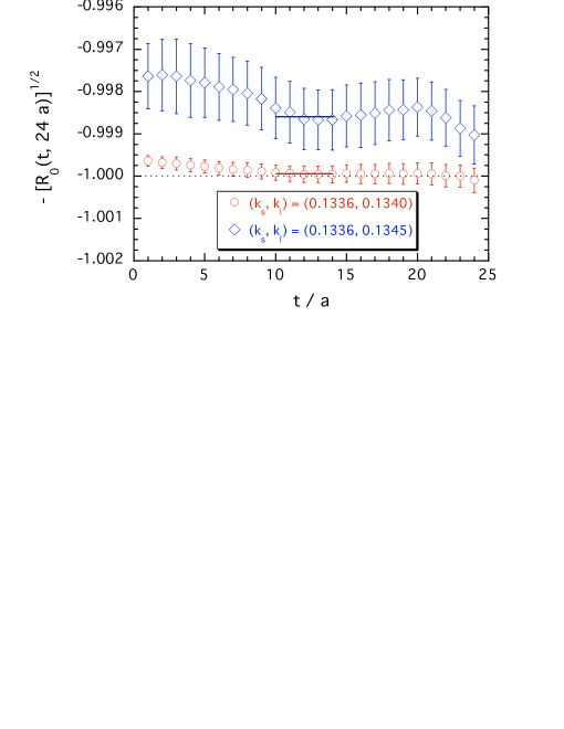
Fig. 1: Time dependence of the quantity $-\sqrt{R_{0}(t,t_{y}=24a)}$, defined in Eq. (26) for the two sets of the hopping parameters, given in the legend. Horizontal bars represent the time interval chosen for the fit.

In Fig. 2 and Table 1 we have collected our results for the quantities $f_{0}(q_{max}^{2})$, determined through the ratio (26), the two mass combinations $a^{2}(M_{\Sigma}^{2}+M_{n}^{2})$ and $a^{2}(M_{\Sigma}^{2}-M_{n}^{2})$, the latter being proportional to the SU(3)-breaking quantity ($m_{s}-m_{\ell}$), and $a^{2}q_{max}^{2}\equiv a^{2}(M_{\Sigma}-M_{n})^{2}$. One can appreciate the remarkable statistical precision obtained for $f_{0}(q_{max}^{2})$, which is always below $0.2\%$: the SU(3)-breaking corrections are clearly resolved with respect to the statistical errors.

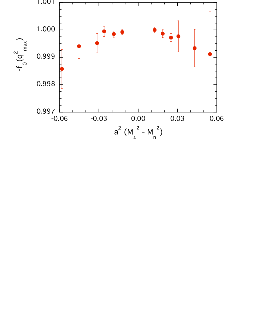
Fig. 2: Results for $[-f_{0}(q^{2}_{max})]$ versus the difference of the squared masses of the external baryons, in lattice units.

$k_{s}-k_{\ell}$	$a^{2}~{}(M_{\Sigma}^{2}+M_{n}^{2})$	$a^{2}~{}(M_{\Sigma}^{2}-M_{n}^{2})$	$a^{2}~{}q_{\rm max}^{2}$	$f_{0}(q_{\rm max}^{2})$
$0.1336-0.1340$	$0.956~{}~{}(9)$	$-0.0261~{}(~{}6)$	$0.000354~{}(17)$	$-0.99995~{}(19)$
$0.1336-0.1343$	$0.937~{}(10)$	$-0.0452~{}(12)$	$0.001086~{}(65)$	$-0.99941~{}(44)$
$0.1336-0.1345$	$0.924~{}(10)$	$-0.0582~{}(17)$	$0.00183~{}~{}(12)$	$-0.99858~{}(71)$
$0.1340-0.1336$	$0.867~{}(12)$	$+0.0250~{}~{}(8)$	$0.000360~{}(24)$	$-0.99972~{}(15)$
$0.1340-0.1343$	$0.824~{}(12)$	$-0.0187~{}~{}(8)$	$0.000211~{}(20)$	$-0.99985~{}(12)$
$0.1340-0.1345$	$0.811~{}(13)$	$-0.0313~{}(14)$	$0.000603~{}(58)$	$-0.99952~{}(36)$
$0.1343-0.1336$	$0.783~{}(15)$	$+0.0431~{}(16)$	$0.001180~{}(99)$	$-0.99933~{}(68)$
$0.1343-0.1340$	$0.759~{}(15)$	$+0.0187~{}~{}(8)$	$0.000229~{}(23)$	$-0.99987~{}(14)$
$0.1343-0.1345$	$0.728~{}(16)$	$-0.0121~{}~{}(8)$	$0.000101~{}(14)$	$-0.99992~{}~{}(9)$
$0.1345-0.1336$	$0.728~{}(18)$	$+0.0548~{}(27)$	$0.00206~{}~{}(22)$	$-0.9991~{}~{}(16)$
$0.1345-0.1340$	$0.704~{}(18)$	$+0.0307~{}(17)$	$0.000666~{}(84)$	$-0.99977~{}(57)$
$0.1345-0.1343$	$0.686~{}(19)$	$+0.0125~{}~{}(8)$	$0.000113~{}(16)$	$-1.00000~{}(11)$

Table 1: Values of the hopping parameters $k_{s}$ and $k_{\ell}$, $a^{2}(M_{\Sigma}^{2}+M_{n}^{2})$, $a^{2}(M_{\Sigma}^{2}-M_{n}^{2})$, $a^{2}q_{\rm max}^{2}\equiv a^{2}(M_{\Sigma}-M_{n})^{2}$ and $f_{0}(q_{\rm max}^{2})$, obtained from the double ratio (26).

Extrapolation to $q^{2}=0$

The next step is to determine both $f_{0}(q^{2})$ and $f_{1}(q^{2})$ for various values of $q^{2}$ using the standard f.f. analysis given by Eqs. (18)-(20). The quality of the plateaux for the quantity $W_{1}(q^{2};t_{x},t_{y})$ (see Eq. (16)), which provides the dominant contribution to $f_{1}(q^{2})$, is shown in Fig. 3. The f.f. $f_{1}(q^{2})$ turns out to be determined with quite good precision as it can be clearly seen in Fig. 4. Note that in Fig. 4 the data points appear paired since both $\Sigma\rightarrow n$ and $n\rightarrow\Sigma$ transitions are considered in the analysis. On the contrary, due to the large statistical noise in the quantities $W_{2}(q^{2};t_{x},t_{y})$ and $W_{3}(q^{2};t_{x},t_{y})$, the results for $f_{0}(q^{2})$ do not share the same level of precision as the one obtained for the f.f. $f_{1}(q^{2})$, a finding similar to what was already observed in Ref. [1] for the $K\to\pi$ transition.

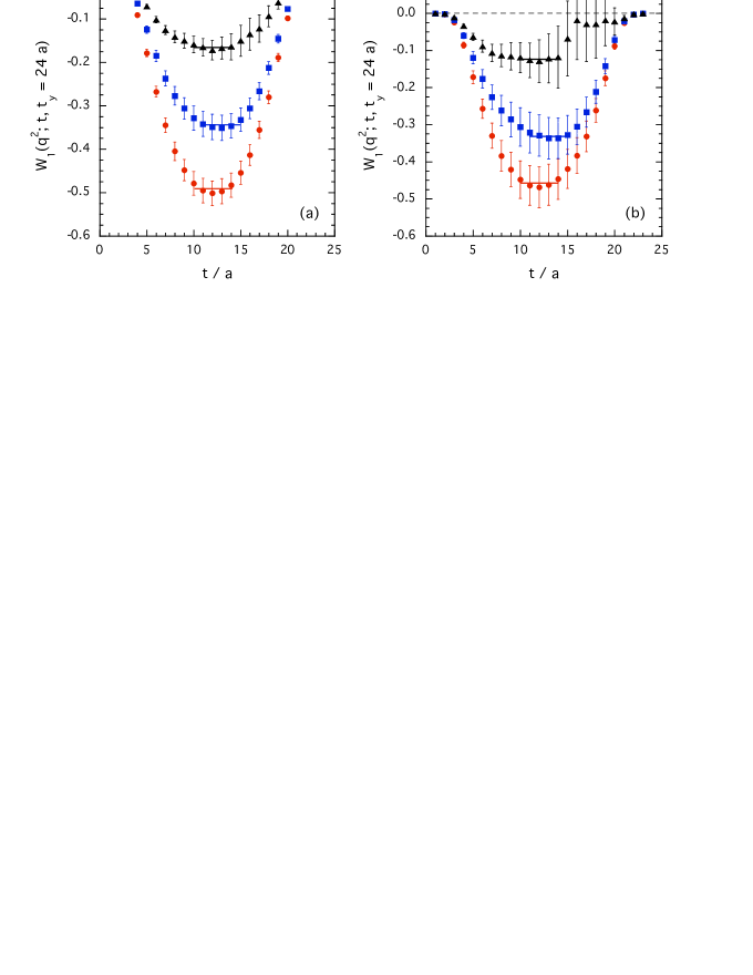
Fig. 3: Time dependence of the quantity $W_{1}(q^{2};t,t_{y}=24a)$ (see Eq. (16)) for the two combinations of the hopping parameters $(k_{s},k_{\ell})=(0.1336,0.1340)$ (a) and $(k_{s},k_{\ell})=(0.1345,0.1343)$ (b). The horizontal bars represent the time intervals chosen for the fit, which provide the value of $\overline{W}_{1}(q^{2})$ (see Eq. (17)). Dots, squares and triangles correspond to $|\vec{q}|^{2}=q_{min}^{2}$, $2q_{min}^{2}$ and $4q_{min}^{2}$, with $q_{min}=2\pi/aL$, respectively.

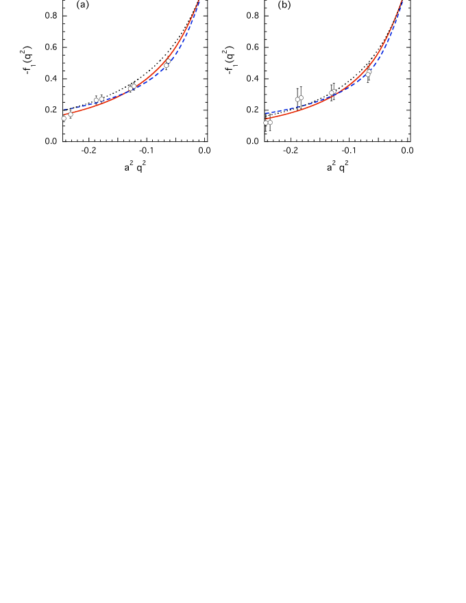
Fig. 4: Values of [$-f_{1}(q^{2})$] versus $a^{2}q^{2}$, as determined by Eq. (18), for the two combinations of the hopping parameters $(k_{s},k_{\ell})=(0.1336,0.1340)$ (a) and $(k_{s},k_{\ell})=(0.1345,0.1343)$ (b). The solid and dashed curves represent the “dipole” and “monopole” fits of Eq. (30), respectively, whereas the dotted curve is a dipole fit with the slope parameter fixed by the $K^{*}$-meson mass.

To improve the determination of $f_{0}(q^{2})$ we introduce the following two double ratios of three-point correlation functions, corresponding to matrix elements of the spatial and time components of the weak vector current:

$$R_{1}(q^{2};t_{x},t_{y}) \equiv \frac{{\rm Im}\left(q_{k}V^{\Sigma n}_{k}(t_{x},t_{y},\vec{q},\vec{0})_{00}\right)}{{\rm Re}\left(V^{\Sigma n}_{0}(t_{x},t_{y},\vec{q},\vec{0})_{00}\right)}\frac{{\rm Re}\left(V^{\Sigma\Sigma}_{0}(t_{x},t_{y},\vec{q},\vec{0})_{00}\right)}{{\rm Im}\left(q_{k}V^{\Sigma\Sigma}_{k}(t_{x},t_{y},\vec{q},\vec{0})_{00}\right)}~{},$$

$$R_{2}(q^{2};t_{x},t_{y}) \equiv \frac{(E_{q}+M_{n}){\rm Im}\left(q_{k}V^{\Sigma n}_{k}\right)+(M_{\Sigma}-M_{n})|\vec{q}|^{2}{\rm Re}\left(V^{\Sigma n}_{2}\right)/q_{1}}{(E_{q}+M_{\Sigma}){\rm Re}\left(V^{\Sigma n}_{0}(t_{x},t_{y},\vec{q},\vec{0})_{00}\right)}$$ (28)

$$\cdot \frac{{\rm Re}\left(V^{\Sigma\Sigma}_{0}(t_{x},t_{y},\vec{q},\vec{0})_{00}\right)}{{\rm Im}\left(q_{k}V^{\Sigma\Sigma}_{k}(t_{x},t_{y},\vec{q},\vec{0})_{00}\right)}~{}.$$

The advantages of the ratios (28) are similar to those already pointed out for the double ratio (26), namely: i) a large reduction of statistical fluctuations; ii) the independence of the renormalization constant $Z_{V}$ and the improvement coefficient $b_{V}$; iii) the cancellation of the dependence on the matrix elements $\sqrt{Z_{\Sigma}}$ and $\sqrt{Z_{n}}$ (see Eq. (16)) between the numerator and the denominator, and iv) $R_{i}(q^{2};t_{x},t_{y})\to 1$ in the SU(3) limit. We stress that the introduction of the matrix elements of degenerate transitions in Eq. (28) is crucial to largely reduce statistical fluctuations, because it compensates the different fluctuations of the matrix elements of the spatial and time components of the weak vector current.

In terms of the large-time limits $\overline{R}_{i}(q^{2})\equiv\mbox{lim}_{\mbox{\tiny$t_{x},(t_{y}-t_{x})\to\infty$}}~{}R_{i}(q^{2};t_{x},t_{y})$ one has

$$\overline{R}_{1}(q^{2}) = \frac{(M_{\Sigma}+M_{n})f_{1}(q^{2})-(E_{q}-M_{n})f_{2}(q^{2})+(E_{q}+M_{\Sigma})f_{3}(q^{2})}{(M_{\Sigma}+M_{n})f_{1}(q^{2})-(E_{q}-M_{\Sigma})f_{2}(q^{2})+(E_{q}-M_{n})f_{3}(q^{2})}~{},$$

$$\overline{R}_{2}(q^{2}) = \frac{(M_{\Sigma}+M_{n})f_{1}(q^{2})-(E_{q}-M_{\Sigma})f_{2}(q^{2})+(E_{q}+M_{n})f_{3}(q^{2})}{(M_{\Sigma}+M_{n})f_{1}(q^{2})-(E_{q}-M_{\Sigma})f_{2}(q^{2})+(E_{q}-M_{n})f_{3}(q^{2})}~{},$$ (29)

which can be solved in terms of $f_{2}(q^{2})/f_{1}(q^{2})$ and $f_{3}(q^{2})/f_{1}(q^{2})$. The latter quantities can be multiplied in turn by the corresponding values of $f_{1}(q^{2})$ evaluated with the standard procedure, obtaining in this way an improved determination of both $f_{2}(q^{2})$ and $f_{3}(q^{2})$, and consequently of $f_{0}(q^{2})$. Our results for $f_{0}(q^{2})$ are shown in Fig. 5, where the very precise lattice point at $q^{2}=q_{max}^{2}$ (the rightmost one), calculated via the double ratio (26), is also reported. It can clearly be seen that the precision achieved for the scalar f.f. $f_{0}(q^{2})$ at $q^{2}\neq q_{max}^{2}$ is comparable to the one obtained for the vector f.f. $f_{1}(q^{2})$ for all the simulated quark masses.

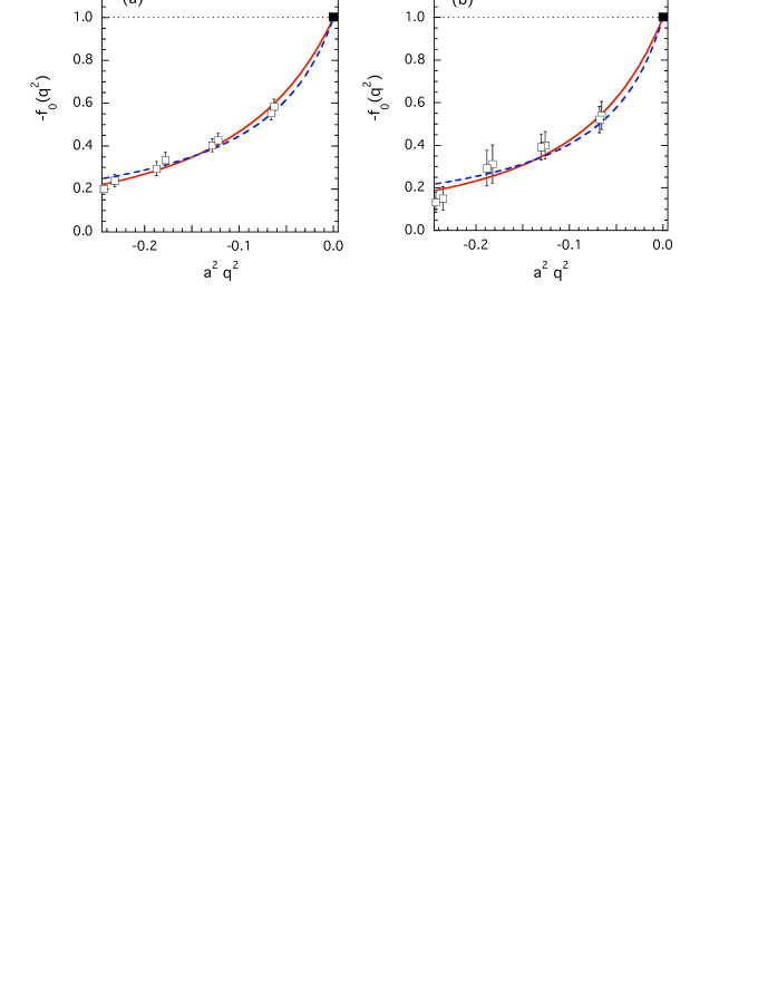
Fig. 5: Values of [$-f_{0}(q^{2})$] versus $a^{2}q^{2}$, calculated using the double ratios (28), for the two combinations of the hopping parameters $(k_{s},k_{\ell})=(0.1336,0.1340)$ (a) and $(k_{s},k_{\ell})=(0.1345,0.1343)$ (b). The full squares represent the very precise lattice point at $q^{2}=q_{max}^{2}$, calculated via the double ratio (26). The dashed and solid curves represent the monopole and dipole fits of Eq. (30), respectively.

The momentum dependence of $f_{0}(q^{2})$ and $f_{1}(q^{2})$ can be analyzed in terms of monopole and dipole behaviors, namely

$$f_{mon.}(q^{2}) = \frac{A}{1-q^{2}/B^{2}}\qquad\qquad\mbox{(monopole fit)},$$

$$f_{dip.}(q^{2}) = \frac{C}{\left(1-q^{2}/D^{2}\right)^{2}}\qquad\qquad\mbox{~{}(dipole fit)}.$$ (30)

As it is clear from Figs. 4 and 5, both functional forms describe the lattice points quite well, with a slightly better quality in the case of the dipole form ($\chi^{2}/d.o.f.~{}\simeq 0.8\div 1.2$ for monopole fits and $\chi^{2}/d.o.f.~{}\simeq 0.6\div 0.8$ for dipole fits). In the case of $f_{1}(q^{2})$, the monopole-fit parameter $B$ turns out to be unrelated to the value predicted by pole dominance (the $K^{*}$-meson mass), while the dipole-fit parameter $D$ agrees with the $K^{*}$-meson mass within $15\%$ accuracy (see dotted lines in Fig. 4). The latter finding is consistent with the experimental determinations of nucleon form factors. Existing data on the proton and neutron form factors are indeed reproduced well either by using a single dipole form with a radius parameter governed by the $\rho$-meson mass, or by several monopole terms corresponding to the dominance of the coupling of the nucleon with $\rho$, $\omega$ and $\phi$ mesons and their resonances [16].

We have applied Eqs. (30) performing a fit to all the lattice points for both $f_{0}(q^{2})$ and $f_{1}(q^{2})$, and imposing the equality $f_{0}(0)=f_{1}(0)$ at zero-momentum transfer. Here below we limit ourselves to present the results obtained in two representative cases, where both $f_{0}(q^{2})$ and $f_{1}(q^{2})$ are assumed to be described either by monopole forms or by dipole ones. Other combinations provide similar results. After fitting the parameters appearing in Eqs. (30) we get the values of $f_{1}(q^{2}=0)$ for the various combinations of quark masses used in the simulation. Our results are collected in Table 2 and plotted in Fig. 6, where they are also compared with those obtained in Ref. [1] in the case of the vector form factor at zero-momentum transfer, $f_{+}(0)$, for the $K_{\ell 3}$ decay.

$k_{s}-k_{\ell}$	$a^{2}(M_{K}^{2}+M_{\pi}^{2})$	$a^{2}(M_{K}^{2}-M_{\pi}^{2})$	$\begin{array}[]{c}f_{1}(0)\\ (monopolefit)\\ \end{array}$	$\begin{array}[]{c}f_{1}(0)\\ (dipolefit)\\ \end{array}$
$0.1336-0.1340$	$0.2819~{}(16)$	$-0.01483~{}(12)$	$-0.9970~{}~{}(4)$	$-0.9976~{}~{}(3)$
$0.1336-0.1343$	$0.2712~{}(17)$	$-0.02557~{}(23)$	$-0.9905~{}(14)$	$-0.9923~{}(11)$
$0.1336-0.1345$	$0.2640~{}(17)$	$-0.03271~{}(28)$	$-0.9835~{}(24)$	$-0.9866~{}(18)$
$0.1340-0.1336$	$0.2529~{}(17)$	$+0.01439~{}(17)$	$-0.9966~{}~{}(5)$	$-0.9972~{}~{}(4)$
$0.1340-0.1343$	$0.2279~{}(17)$	$-0.01061~{}(15)$	$-0.9979~{}~{}(4)$	$-0.9983~{}~{}(3)$
$0.1340-0.1345$	$0.2209~{}(18)$	$-0.01758~{}(18)$	$-0.9939~{}(11)$	$-0.9951~{}~{}(9)$
$0.1343-0.1336$	$0.2209~{}(18)$	$+0.02464~{}(14)$	$-0.9875~{}(24)$	$-0.9902~{}(18)$
$0.1343-0.1340$	$0.2068~{}(18)$	$+0.01050~{}(10)$	$-0.9975~{}~{}(5)$	$-0.9981~{}~{}(4)$
$0.1343-0.1345$	$0.1895~{}(18)$	$-0.00676~{}(10)$	$-0.9989~{}~{}(3)$	$-0.9991~{}~{}(2)$
$0.1345-0.1336$	$0.2002~{}(19)$	$+0.03111~{}(17)$	$-0.9766~{}(60)$	$-0.9818~{}(45)$
$0.1345-0.1340$	$0.1862~{}(19)$	$+0.01714~{}(13)$	$-0.9925~{}(22)$	$-0.9942~{}(17)$
$0.1345-0.1343$	$0.1759~{}(19)$	$+0.00685~{}~{}(9)$	$-0.9988~{}~{}(4)$	$-0.9991~{}~{}(3)$

Table 2: Values of the hopping parameters $k_{s}$ and $k_{\ell}$, $a^{2}(M_{K}^{2}+M_{\pi}^{2})$, $a^{2}(M_{K}^{2}-M_{\pi}^{2})$ and $f_{1}(q^{2}=0)$, obtained assuming either a monopole or a dipole momentum dependence of both $f_{0}(q^{2})$ and $f_{1}(q^{2})$ to perform the extrapolation to $q^{2}=0$ [see Eqs. (30)].

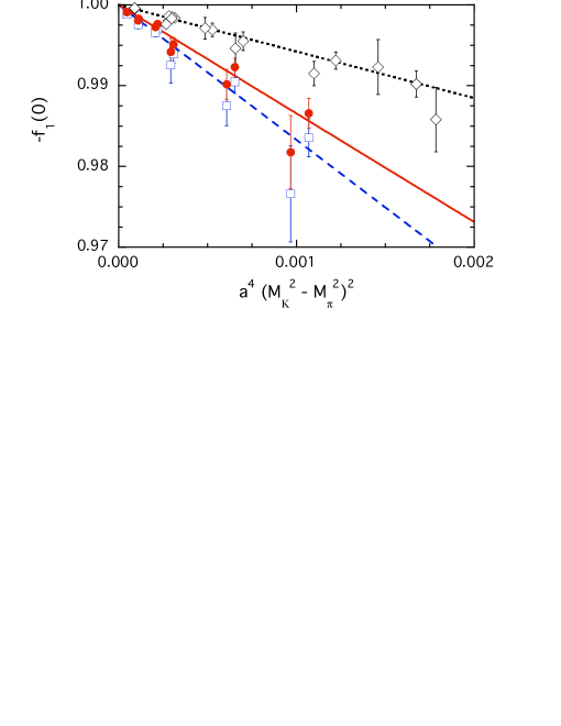
Fig. 6: Results for [$-f_{1}(0)$] vs. the mass difference $a^{4}(M_{K}^{2}-M_{\pi}^{2})^{2}$, obtained after extrapolation to $q^{2}=0$ through either monopole (open squares) or dipole (full circles) fits to the lattice points for $f_{0}(q^{2})$ and $f_{1}(q^{2})$ (see Eqs. (30)). The open diamonds are the results obtained in Ref. [1] for the vector form factor at zero-momentum transfer, $f_{+}(0)$, corresponding to the $K_{\ell 3}$ decay. The dotted, dashed and solid lines are linear fits to the data, according to the AG theorem.

In agreement with the Ademollo-Gatto theorem our results for hyperon semileptonic decays exhibit an approximate linear behavior in the quadratic SU(3)-breaking parameter $(M_{K}^{2}-M_{\pi}^{2})^{2}\propto(m_{s}-m_{\ell})^{2}$, as shown in Fig. 6. Note that:   i) the amount of SU(3) breaking in the vector form factor at zero-momentum transfer appears to be larger in the hyperon case with respect to the $K_{\ell 3}$ decay;   ii) the statistical uncertainty on $f_{1}(0)$ is in the range $0.02\div 0.6\%$ at the simulated quark masses, and   iii) lattice artifacts on $f_{1}(0)$ due to the finiteness of the lattice spacing start at ${\cal O}(a^{2})$ and are proportional to $(m_{s}-m_{\ell})^{2}$, like the physical SU(3)-breaking effects; we therefore expect that, by having in our lattice simulation $a^{-1}\simeq 2.6$ GeV, discretization errors are sensibly smaller than the physical SU(3)-breaking effects. Further investigations at different values of the lattice spacing could better clarify this point.

Chiral extrapolation

Following Ref. [1] we construct the AG ratio defined as

$$R(M_{K},M_{\pi})\equiv\frac{1+f_{1}(0)}{a^{4}~{}(M_{K}^{2}-M_{\pi}^{2})^{2}}~{},$$ (31)

in which the leading meson mass dependence predicted by the AG theorem is factorized out. This quantity depends on both kaon and pion masses, or equivalently on the two independent mass combinations $a^{2}(M_{K}^{2}+M_{\pi}^{2})$ and $a^{2}(M_{K}^{2}-M_{\pi}^{2})$. As shown in Fig. 7, the dependence of the AG ratio (31) on the meson masses is well described by a simple linear fit:

$$R(M_{K},M_{\pi})=R_{0}+R_{1}\cdot a^{2}(M_{K}^{2}+M_{\pi}^{2})~{},$$ (32)

whereas the dependence upon the variable $a^{2}(M_{K}^{2}-M_{\pi}^{2})$ is found to be negligible. In order to investigate the stability of extrapolation to the physical point we consider also a quadratic fit in the meson masses:

$$R(M_{K},M_{\pi})=\tilde{R}_{0}+\tilde{R}_{1}\cdot a^{2}(M_{K}^{2}+M_{\pi}^{2})+\tilde{R}_{2}\cdot a^{4}(M_{K}^{2}+M_{\pi}^{2})^{2}~{}.$$ (33)

The consequent increase of the number of parameters leads to larger uncertainties, while the shift in the central values remains at the level of the statistical errors.

The extrapolation of $R(M_{K},M_{\pi})$ to the physical point is performed using the physical values of meson masses in lattice units calculated by fixing the ratios $M_{K}/M_{K^{*}}$ and $M_{\pi}/M_{\rho}$ to their experimental values, obtaining

$$[aM_{K}]^{\rm phys}=0.189(2)~{}, [aM_{\pi}]^{\rm phys}=0.0536(7)~{}.$$ (34)

From Fig. 7 it can clearly be seen that:

• as already observed, the AG ratio for hyperon decay is $\simeq 2\div 3$ times larger than the corresponding ratio obtained for the $K_{\ell 3}$ decay in Ref. [1];

• the minimum value of $a^{2}(M_{K}^{2}+M_{\pi}^{2})$ reached in our calculations is two times larger than the corresponding minimum value achieved in the case of the $K_{\ell 3}$ decay. The reason is that the quality of the signal coming from the ground state depends on the energy gap between the ground and the excited states (sharing the same quantum numbers). As the quark mass decreases, the energy gap slightly decreases in the case of hyperons [17], while it increases in the case of pseudoscalar mesons. The net result is an increase of the statistical errors at large-time distances, which is more pronounced in the case of hyperons with respect to the case of pseudoscalar mesons. Note also that we have adopted single, local interpolating fields for hyperons (see Eq. (6)). The use of smeared source and sink, as well as the use of several, independent interpolating fields may help in achieving a better isolation of the ground-state signal.

Since in our simulation quark masses are rather large, we expect that the effects of pseudoscalar meson loops may be suppressed, which means that chiral logarithms are unlikely to affect significantly the lattice results. The analog case of the $K\to\pi$ transition, in which the leading chiral corrections in the quenched approximation have been explicitly evaluated [1], shows indeed that their contributions are almost negligible at the quark masses used in the simulation, as it is illustrated in Fig. 7 (compare full diamonds with open squares). Therefore our results for the AG ratio of the vector f.f. should be considered mainly as an estimate of the contributions from local terms in the chiral expansion. We then extrapolate the lattice results to the physical values of the meson masses by assuming a simple polynomial dependence, as in Eqs. (32) and (33). Effects of meson loops, evaluated in full QCD at the physical quark masses, should be eventually added. Their impact and the actual limitations of HBChPT will be discussed in the next Section. We also note that, in the case of $K_{\ell 3}$ decays, preliminary results of unquenched simulations [2] seem to indicate the smallness of quenching effects.

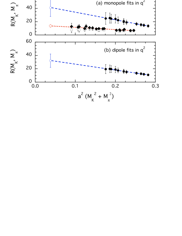
Fig. 7: Values of the AG ratio $R(M_{K},M_{\pi})$ versus the mass combination $a^{2}(M_{K}^{2}+M_{\pi}^{2})$, for the cases of the monopole and dipole fits of both $f_{0}(q^{2})$ and $f_{1}(q^{2})$. The dashed lines represent the results of the linear fit (32), while the open dots indicate the value of the AG ratio extrapolated to the physical point. In (a) the full diamonds and the open squares are the corresponding results obtained for the AG ratio in the case of the $K_{\ell 3}$ decay in Ref. [1] with and without the subtraction of the leading chiral correction, respectively.

In Table 3 we collect the extrapolated values $R(M_{K}^{\rm phys.},M_{\pi}^{\rm phys.})$ obtained for the various functional forms assumed in fitting both the $q^{2}$-dependence of the form factors (Eq. (30)) and the meson mass dependence given by Eqs. (32)-(33). Two sets of results are presented in Table 3. The first set, given in the upper table, is obtained by determining the matrix elements $\sqrt{Z_{\Sigma}}$ and $\sqrt{Z_{n}}$ (see Eq. (16)) from a fit of the two-point correlation functions in the same time interval chosen for the three-point correlators, namely $t/a\in$ [10,16]. For the second set, given in the lower table, the same time interval chosen to extract hadron masses, i.e. $t/a\in$ [19,25], has been considered. Note that the uncertainties in the extrapolated value $R(M_{K}^{\rm phys.},M_{\pi}^{\rm phys.})$ turn out to be quite large mostly because of the long chiral extrapolation. Simulations at lower quark masses would be very beneficial in reducing such an uncertainty.

$R(M_{K}^{\rm phys.},M_{\pi}^{\rm phys.})$	Linear Fit	Quadratic Fit
Monopole fits in $q^{2}$	$41\pm 13$	$52\pm 29$
Dipole fits in $q^{2}$	$32\pm 10$	$35\pm 30$

$R(M_{K}^{\rm phys.},M_{\pi}^{\rm phys.})$	Linear Fit	Quadratic Fit
Monopole fits in $q^{2}$	$55\pm 19$	$78\pm 39$
Dipole fits in $q^{2}$	$40\pm 13$	$49\pm 35$

Table 3: Results for the AG ratio at the physical point, $R(M_{K}^{\rm phys.},M_{\pi}^{\rm phys.})$, obtained from linear (32) or quadratic (33) fits in the meson masses, assuming either monopole or dipole functional forms for the extrapolation of the scalar $f_{0}(q^{2})$ and vector $f_{1}(q^{2})$ form factors to $q^{2}=0$. Upper and lower tables correspond to different choices of the time interval chosen for the fits of the two-point correlation functions (see text).

From the spread of the results given in Table 3 we quote $R(M_{K}^{\rm phys.},M_{\pi}^{\rm phys.})=48\pm 14_{\rm stat.}\pm 23_{\rm syst.}$, which implies

$$1+f_{1}(0) = R(M_{K}^{\rm phys.},M_{\pi}^{\rm phys.})\cdot\left[(aM_{K}^{\rm phys.})^{2}-(aM_{\pi}^{\rm phys.})^{2}\right]^{2}$$ (35)

$$= 0.052\pm 0.015_{\rm stat.}\pm 0.025_{syst.}=(5.2\pm 2.9)\%~{},$$

where the systematic error includes the uncertainties due to the extrapolation in $q^{2}$ and in the meson masses, while it does not include the uncertainty due to the quenching effects. In addition, the result (35) does not include the effects of chiral logarithms induced by meson loops, which will be discussed in the next Section.

4 Chiral corrections in HBChPT

The chiral behavior of the vector form factor at zero-momentum transfer $f_{1}(0)$ has been recently investigated in Ref. [7] using HBChPT, where baryons are treated as heavy degrees of freedom and a $1/M_{B}$ expansion around the non-relativistic limit is performed. The chiral corrections to $f_{1}(0)$ can be schematically expressed as

$$f_{1}(0)=f_{1}^{SU(3)}(0) \cdot \left\{1+{\cal O}\left(\frac{M_{K}^{2}}{(4\pi f_{\pi})^{2}}\right)+{\cal O}\left(\frac{M_{K}^{2}}{(4\pi f_{\pi})^{2}}\frac{\pi\delta M_{B}}{M_{K}}\right)+\right.$$ (36)

$$~{}\left.{\cal O}\left(\frac{M_{K}^{2}}{(4\pi f_{\pi})^{2}}\frac{\pi M_{K}}{M_{B}}\right)+O(p^{4})\right\}~{},$$

where $f_{1}^{SU(3)}(0)$ is the value of $f_{1}(0)$ in the SU(3) limit which is fixed by the vector current conservation. In the r.h.s. of Eq. (36) the second term in the brackets represents the one-loop ${\cal O}(p^{2})$ correction, while the subsequent two terms are the (parametrically) sub-leading ${\cal O}(p^{3})$ and ${\cal O}(1/M_{B})$ corrections, respectively. The various chiral corrections in Eq. (36) have been computed in Ref. [7], which completes and corrects previous determinations presented in the literature [18, 19]. The corresponding numerical estimates are collected in Table 4 for various hyperon decays. An important feature of the chiral expansion (36) is that the ${\cal O}(p^{2})$, ${\cal O}(p^{3})$ and ${\cal O}(1/M_{B})$ corrections are independent from unknown LECs thanks to the AG theorem.

$f_{1}(0)/f_{1}^{SU(3)}(0)$	$f_{1}^{SU(3)}(0)$	${\cal O}(p^{2})$	${\cal O}(p^{3})$	${\cal O}(1/M_{B})$	All
$\Sigma^{-}\to n$	$-1$	$+0.7$%	$+6.5$%	$-3.2$%	$+4.1$%
$\Lambda\to p$	$-\sqrt{3/2}$	$-9.5$%	$+4.3$%	$+8.0$%	$+2.7$%
$\Xi^{-}\to\Lambda$	$\sqrt{3/2}$	$-6.2$%	$+6.2$%	$+4.3$%	$+4.3$%
$\Xi^{-}\to\Sigma^{0}$	$1/\sqrt{2}$	$-9.2$%	$+2.4$%	$+7.7$%	$+0.9$%

Table 4: Chiral corrections at the physical point estimated in Ref. [7] for various hyperon decays.

The sum of all the contributions for $f_{1}(0)/f_{1}^{SU(3)}(0)$, presented in Table 4, turns out to be positive and of the order of few percent for the various hyperon decays considered. However the final results come from partial cancellation of larger terms. Thus higher order corrections are expected to give non-negligible contributions, and the convergence of the chiral expansion for hyperon transitions turns out to be questionable [7].

In addition an important source of uncertainty is represented by the mixing with the $J^{P}=3/2^{+}$ decuplet in the effective field theory calculations. If the mass-shift $\Delta$ between the decuplet and the octet hyperons were much larger than the interaction scale $\Lambda_{QCD}$, the decuplet contribution could be integrated out and reabsorbed into the LECs, so that no correction would appear up to ${\cal O}(p^{3})$ in the chiral expansion. However $\Delta\simeq 230~{}{\rm MeV}$ is of order $\Lambda_{QCD}$ and therefore the decuplet may give non-negligible, non-analytic contributions to the chiral expansion.

The HBChPT with explicit decuplet degrees of freedom was firstly proposed in Ref. [20] and formalized as an expansion in Ref. [21]. Its impact at ${\cal O}(p^{2})$, ${\cal O}(p^{3})$ and ${\cal O}(1/M_{B})$ has been investigated in Ref. [7]. As for the octet contributions, the AG theorem protects the decuplet corrections from unknown LECs and the only new parameter, besides $\Delta$, is the known decuplet–octet–meson coupling ${\cal C}\simeq 1.6$ [22]. At ${\cal O}(p^{2})$ the dynamical decuplet gives an important contribution to the $\Sigma^{-}\to n$ transition ($-3.1$%). At ${\cal O}(p^{3})$ there are two contributions. The first one is due to the insertion of decuplet mass-shifts and it is of order $-1.8$%. The second contribution is due to baryon mass-shift insertions and gives a huge contribution of about $-38$%. This effect completely breaks the chiral expansion raising serious doubts on the consistency of the HBChPT with dynamical decuplet. The reason why this effect was not noticed before is because other quantities, at this order, contain a large number of LECs which are difficult to estimate from the data. In the case of $f_{1}(0)$ there are no LECs and a true test of the convergence of the chiral expansion is possible.

It is therefore clear that a model-independent estimate of chiral corrections for hyperon decays cannot be given at present. We can limit ourselves to trust HBChPT without dynamical decuplet, making the Ansatz that the decuplet contributions can be reabsorbed into local terms. Under this assumption the chiral correction to $f_{1}(0)$ for the $\Sigma^{-}\to n$ transition can be estimated from Table 4 to be $(-4\pm 4)\%$, assuming a $100\%$ overall uncertainty. Thus (at least) in the case of the $\Sigma^{-}\to n$ transition there seems to be a partial cancellation between chiral loop corrections from the HBChPT and local contributions from the lattice calculation, Eq. (35), though within quite large uncertainties. Adding the two results we get

$$f_{1}(0)=-0.988\pm 0.029_{\rm lattice}\pm 0.040_{\rm HBChPT}~{}.$$ (37)

Unquenched simulations with light quark masses are required to provide a reliable estimate of SU(3)-breaking corrections to hyperon form factors without relying on the chiral expansion.

5 Results for $g_{1}(0)/f_{1}(0)$

The ratio of the axial to the vector f.f. at zero-momentum transfer, $g_{1}(0)/f_{1}(0)$, is an important ingredient in the analysis of experimental data on hyperon semileptonic decays (see Refs. [3] and [23]). In this Section we first present the lattice results for the momentum dependence of the ratio $g_{1}(q^{2})/f_{1}(q^{2})$, then we extrapolate it in $q^{2}$ down to $q^{2}=0$ and finally we analyze its mass dependence to obtain the ratio $g_{1}(0)/f_{1}(0)$ at the physical quark masses.

Using the standard procedure, the two f.f.’s $g_{1}(q^{2})$ and $f_{1}(q^{2})$ can be separately calculated for $\vec{q}\neq 0$ through Eqs. (23) and (18) in terms of the quantities $\overline{W}_{i}^{(A)}(q^{2})$ and $\overline{W}_{j}(q^{2})$ ($i,j=1,2,3$), defined in Eqs. (22) and (17), respectively. In this way one obtains values of $g_{1}(q^{2})$ with a statistical precision similar to the one achieved for the f.f. $f_{1}(q^{2})$.

A reduction of the statistical noise can be obtained by considering directly the quantity $g_{1}(q^{2})/f_{1}(q^{2})$ in terms of the ratios $\overline{W}_{i}^{(A)}(q^{2})/\overline{W}_{j}(q^{2})$. In this way the statical noise introduced by the two-point correlation functions in the denominators of Eqs. (21) and (16) is cancelled out. Moreover, also the systematic uncertainty due to different ways of determining the matrix elements $\sqrt{Z_{\Sigma}}$ and $\sqrt{Z_{n}}$ (typically a $\simeq 10\%$ effect) is removed. The values of $g_{1}(q^{2})/f_{1}(q^{2})$ obtained at $\vec{q}\neq 0$ (i.e., $q^{2}\neq q_{max}^{2}$) are shown in Fig. 8 for two combinations of quark masses.

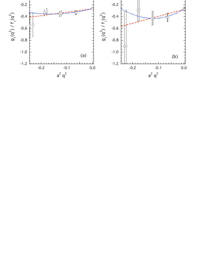
Fig. 8: Values of $g_{1}(q^{2})/f_{1}(q^{2})$ versus $a^{2}q^{2}$, obtained for the two combinations of the hopping parameters $(k_{s},k_{\ell})=(0.1336,0.1340)$ (a) and $(k_{s},k_{\ell})=(0.1345,0.1343)$ (b). The dashed and dotted lines represent linear and quadratic fits in $q^{2}$, respectively.

At $\vec{q}=0$, corresponding to $q^{2}=q_{max}^{2}$, neither $g_{1}$ nor $f_{1}$ can be calculated directly. For both initial and final hyperons at rest there are only two non-vanishing matrix elements with $\gamma=\gamma^{\prime}=0$, ${\rm Im}\left(A_{3}^{\Sigma n}(t_{x},t_{y},\vec{0},\vec{0})_{00}\right)$ and ${\rm Re}\left(V_{0}^{\Sigma n}(t_{x},t_{y},\vec{0},\vec{0})_{00}\right)$. Their ratio provides a new combination of f.f.’s, namely

$$\frac{{\rm Im}\left(A_{3}^{\Sigma n}(t_{x},t_{y},\vec{0},\vec{0})_{00}\right)}{{\rm Re}\left(V_{0}^{\Sigma n}(t_{x},t_{y},\vec{0},\vec{0})_{00}\right)}=\frac{g_{1}(q_{max}^{2})+\frac{M_{\Sigma}-M_{n}}{M_{\Sigma}+M_{n}}g_{2}(q_{max}^{2})}{f_{1}(q_{max}^{2})+\frac{M_{\Sigma}-M_{n}}{M_{\Sigma}+M_{n}}f_{3}(q_{max}^{2})}\equiv\frac{\tilde{g}_{1}(q_{max}^{2})}{f_{0}(q_{max}^{2})}~{}.$$ (38)

To get $g_{1}(q_{max}^{2})/f_{1}(q_{max}^{2})$ we apply two corrections to Eq. (38). The first one corresponds to multiply the values of $\tilde{g}_{1}(q_{max}^{2})/f_{0}(q_{max}^{2})$ by $f_{0}(q_{max}^{2})/f_{1}(q_{max}^{2})$, where the values of $f_{0}(q_{max}^{2})$ are obtained with the double ratio (26), while those for $f_{1}(q_{max}^{2})$ can be evaluated using the dipole fit of Eqs. (30). The second correction is the subtraction of the contribution due to $g_{2}(q_{max}^{2})/f_{1}(q_{max}^{2})$, whose values can be obtained by fitting the momentum dependence of the ratio $g_{2}(q^{2})/f_{1}(q^{2})$ (see next Section). Thanks to the smallness of the difference $M_{\Sigma}-M_{n}$ in our simulation, both corrections turn out to be much smaller than the statistical errors, so that the ratio (38) can be safely corrected providing a determination of $g_{1}(q_{max}^{2})/f_{1}(q_{max}^{2})$ with quite good statistical precision ($\lesssim 10\%$), as it is shown by the rightmost point in Fig. 8.

The addition of a precise determination at $q^{2}=q_{max}^{2}$ is crucial to improve the extrapolation to $q^{2}=0$. Indeed, thanks to the closeness of the $q_{max}^{2}$ values to $q^{2}=0$, the extrapolated values $g_{1}(0)/f_{1}(0)$ are only slightly affected by the specific functional form adopted for describing the momentum dependence of $g_{1}(q^{2})/f_{1}(q^{2})$, as it is can be clearly seen from Fig. 8. In Table 5 and in Fig. 9 we show the results obtained for $g_{1}(0)/f_{1}(0)$ using a linear fit in $q^{2}$.

$k_{s}-k_{\ell}$	$g_{1}(0)/f_{1}(0)$
$0.1336-0.1340$	$-0.266~{}(18)$
$0.1336-0.1343$	$-0.261~{}(19)$
$0.1336-0.1345$	$-0.257~{}(19)$
$0.1340-0.1336$	$-0.273~{}(20)$
$0.1340-0.1343$	$-0.267~{}(22)$
$0.1340-0.1345$	$-0.264~{}(22)$
$0.1343-0.1336$	$-0.273~{}(22)$
$0.1343-0.1340$	$-0.275~{}(23)$
$0.1343-0.1345$	$-0.270~{}(26)$
$0.1345-0.1336$	$-0.274~{}(27)$
$0.1345-0.1340$	$-0.278~{}(28)$
$0.1345-0.1343$	$-0.279~{}(31)$

Table 5: Values of the ratio $g_{1}(0)/f_{1}(0)$, obtained from a linear fit in $q^{2}$ of the lattice results for $g_{1}(q^{2})/f_{1}(q^{2})$.

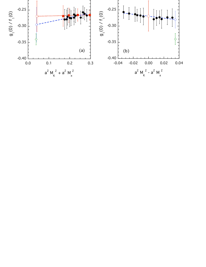
Fig. 9: Results for the ratio $g_{1}(0)/f_{1}(0)$ vs. the meson mass combinations $a^{2}(M_{K}^{2}+M_{\pi}^{2})$ (a) and $a^{2}(M_{K}^{2}-M_{\pi}^{2})$ (b), obtained after extrapolation to $q^{2}=0$ through linear fits in $q^{2}$. Full dots and squares correspond to lattice results calculated with non-degenerate and degenerate quark masses, respectively (i.e. with and without SU(3)-breaking corrections). The dashed and dotted lines are linear fits in the meson masses putting in Eq. (39) $A_{2}=0$ (a) and $A_{1}=0$ (b), while the open dot and square are the corresponding values extrapolated to the physical point. The diamond represents the value of the ratio $g_{1}(0)/f_{1}(0)$ adopted in Ref. [3].

Since the axial-vector f.f. at zero-momentum transfer, $g_{1}(0)$, is not protected by the AG theorem against first-order corrections in the SU(3)-breaking parameter $(m_{s}-m_{\ell})\propto a^{2}(M_{K}^{2}-M_{\pi}^{2})$, we start the analysis of the mass dependence of $g_{1}(0)/f_{1}(0)$ by considering a linear fit in the two mass combinations $a^{2}(M_{K}^{2}+M_{\pi}^{2})$ and $a^{2}(M_{K}^{2}-M_{\pi}^{2})$:

$$\frac{g_{1}(0)}{f_{1}(0)}=A_{0}+A_{1}\cdot a^{2}(M_{K}^{2}+M_{\pi}^{2})+A_{2}\cdot a^{2}(M_{K}^{2}-M_{\pi}^{2})~{}.$$ (39)

The resulting values of the parameters are: $A_{0}=-0.281~{}(59)$, $A_{1}=0.05~{}(20)$ and $A_{2}=-0.25~{}(12)$, which provide at the physical meson masses the value

$$\left[\frac{g_{1}(0)}{f_{1}(0)}\right]^{phys.}=-0.287\pm 0.052~{},$$ (40)

where the error does not include the quenching effect. Assuming $A_{2}=0$ one gets $A_{0}=-0.300~{}(61)$, $A_{1}=0.14~{}(21)$ with $[g_{1}(0)/f_{1}(0)]^{phys.}=-0.295\pm 0.053$, whereas adopting $A_{1}=0$ one gets $A_{0}=-0.270~{}(21)$, $A_{2}=-0.30~{}(26)$ with $[g_{1}(0)/f_{1}(0)]^{phys.}=-0.280\pm 0.026$. In both cases the values extrapolated to the physical point agree with the result given by Eq. (40) within the statistical errors. The two separate linear fits in the mass combinations $a^{2}(M_{K}^{2}+M_{\pi}^{2})$ and $a^{2}(M_{K}^{2}-M_{\pi}^{2})$ are shown in Fig. 9 by the dashed lines. We have checked that the results presented for $[g_{1}(0)/f_{1}(0)]^{phys.}$ remain unchanged if instead of the meson masses the hyperon ones are adopted in the fitting procedure based on the Ansatz (39). We also tried quadratic fits in the mass combinations $a^{2}(M_{K}^{2}+M_{\pi}^{2})$ and $a^{2}(M_{K}^{2}-M_{\pi}^{2})$. The consequent increase of the number of parameters leads to larger uncertainties, but the shift in the central values remains smaller than the statistical errors.

The case of degenerate quark masses $m_{s}=m_{\ell}$ (i.e., $q_{max}^{2}=0$) allows us to access directly the values of $g_{1}(0)/f_{1}(0)$ in the case of exact SU(3) symmetry. Without any extrapolation in $q^{2}$ we obtain the four values of $g_{1}(0)/f_{1}(0)$ shown in Fig. 9(a) by the full dots. A linear extrapolation in the squared pion mass gives

$$\left[\frac{g_{1}(0)}{f_{1}(0)}\right]_{SU(3)}^{phys.}=-0.269\pm 0.047~{},$$ (41)

which nicely agrees with the prediction of the linear fit shown in Fig. 9(b) at the SU(3)-symmetric point $a^{2}(M_{K}^{2}-M_{\pi}^{2})=0$. The comparison with result (40) indicates that at the physical point the ratio $g_{1}(0)/f_{1}(0)$ is affected by moderate SU(3)-breaking corrections, though it is not protected by the AG theorem. Our finding is in qualitative agreement with the exact SU(3)-symmetry assumption of the Cabibbo model [9].

Our result (40) is also consistent within the errors with the value $g_{1}(0)/f_{1}(0)=-0.340\pm 0.017$ adopted in the recent analysis of hyperon decays of Ref. [3], where the exact SU(3)-symmetry assumption for the ratio $g_{1}(0)/f_{1}(0)$ is avoided.

6 Results for the other form factors

In this Section we analyze the momentum dependence of the ratios of the remaining f.f.’s $f_{2}(q^{2})$, $g_{2}(q^{2})$, $f_{3}(q^{2})$ and $g_{3}(q^{2})$ to the vector f.f. $f_{1}(q^{2})$. The contributions of both $f_{3}(q^{2})$ and $g_{3}(q^{2})$ to the decay distributions are suppressed by the ratio of the lepton to the hyperon mass, and therefore they are negligible in the case of hyperon decays with electrons, while they can be relevant for muonic decays. The latter however suffer from quite small branching ratios [23].

As described in Section 3 the ratios $f_{2}(q^{2})/f_{1}(q^{2})$ and $f_{3}(q^{2})/f_{1}(q^{2})$ can be calculated using the double ratios (28)-(29). The latter can be easily generalized to the axial sector to determine the ratios $g_{2}(q^{2})/f_{1}(q^{2})$ and $g_{3}(q^{2})/f_{1}(q^{2})$. We introduce the following two double ratios of three-point correlation functions, corresponding to matrix elements of spatial and time components of the weak axial current:

$$R_{1}^{(A)}(q^{2};t_{x},t_{y}) \equiv \frac{{\rm Re}\left(A_{0}^{\Sigma n}(t_{x},t_{y},\vec{q},\vec{0})_{00}\right)}{{\rm Im}\left(\tilde{A}^{\Sigma n}(t_{x},t_{y},\vec{q},\vec{0})_{00}\right)}\frac{{\rm Im}\left(\tilde{A}^{\Sigma\Sigma}(t_{x},t_{y},\vec{q},\vec{0})_{00}\right)}{{\rm Re}\left(A_{0}^{\Sigma\Sigma}(t_{x},t_{y},\vec{q},\vec{0})_{00}\right)}~{},$$

$$R_{2}^{(A)}(q^{2};t_{x},t_{y}) \equiv \frac{{\rm Re}\left(A_{0}^{\Sigma n}\right)+(M_{n}-M_{\Sigma})~{}{\rm Im}\left(A^{\Sigma n}_{1}\right)/q_{1}}{{\rm Re}\left(A^{\Sigma n}_{0}(t_{x},t_{y},\vec{q},\vec{0})_{00}\right)}$$ (42)

$$\cdot \frac{{\rm Im}\left(\tilde{A}^{\Sigma\Sigma}(t_{x},t_{y},\vec{q},\vec{0})_{00}\right)}{{\rm Re}\left(A_{0}^{\Sigma\Sigma}(t_{x},t_{y},\vec{q},\vec{0})_{00}\right)}~{}.$$

We emphasize that the ratios (42) are exactly equal to unity in the SU(3) limit, and therefore the deviation of these ratios from one are a measure of SU(3)-breaking corrections. This is crucial for obtaining a determination of f.f.’s like the weak electricity $g_{2}(q^{2})$ (and the induced scalar $f_{3}(q^{2})$ in the vector case), which vanish identically in the SU(3) limit.

In terms of the large-time limits $\overline{R}_{i}^{(A)}(q^{2})\equiv\mbox{lim}_{\mbox{\tiny$t_{x},(t_{y}-t_{x})\to\infty$}}~{}R_{i}^{(A)}(q^{2};t_{x},t_{y})$ one has

$$\overline{R}_{1}^{(A)}(q^{2}) = \frac{(M_{\Sigma}+M_{n})g_{1}(q^{2})-(E_{q}+M_{\Sigma})g_{2}(q^{2})+(E_{q}-M_{n})g_{3}(q^{2})}{(M_{\Sigma}+M_{n})g_{1}(q^{2})-(E_{q}-M_{n})g_{2}(q^{2})+(E_{q}-M_{\Sigma})g_{3}(q^{2})}~{},$$

$$\overline{R}_{2}^{(A)}(q^{2}) = \frac{(M_{\Sigma}+M_{n})g_{1}(q^{2})-(E_{q}+M_{n})g_{2}(q^{2})+(E_{q}-M_{\Sigma})g_{3}(q^{2})}{(M_{\Sigma}+M_{n})g_{1}(q^{2})-(E_{q}-M_{n})g_{2}(q^{2})+(E_{q}-M_{\Sigma})g_{3}(q^{2})}~{},$$ (43)

which can be can be easily solved in terms of $g_{2}(q^{2})/g_{1}(q^{2})$ and $g_{3}(q^{2})/g_{1}(q^{2})$. The latter can be multiplied in turn by the values of $g_{1}(q^{2})/f_{1}(q^{2})$ to get the ratios $g_{2}(q^{2})/f_{1}(q^{2})$ and $g_{3}(q^{2})/f_{1}(q^{2})$.

The study of the momentum dependence of the four ratios $f_{2}(q^{2})/f_{1}(q^{2})$, $f_{3}(q^{2})/f_{1}(q^{2})$, $g_{2}(q^{2})/f_{1}(q^{2})$ and $g_{3}(q^{2})/f_{1}(q^{2})$ suffers however of a crucial difference with respect to the case of the ratio $g_{1}(q^{2})/f_{1}(q^{2})$, namely the absence of a determination at $q^{2}=q_{max}^{2}$ and, in general, of a lattice point sufficiently close to $q^{2}=0$. This limitation makes the extrapolation to $q^{2}=0$ plagued by larger uncertainties. A way to cure this problem may be the use of twisted boundary conditions for the quark fields [24]. Indeed, as shown in Ref. [25], non-periodic boundary conditions may greatly help in determining form factors at zero-momentum transfer, when the latter cannot be determined sufficiently close to $q^{2}=0$ using periodic boundary conditions.

We discuss first the ratios $f_{2}(q^{2})/f_{1}(q^{2})$ and $g_{3}(q^{2})/f_{1}(q^{2})$, and then the ratios $g_{2}(q^{2})/f_{1}(q^{2})$ and $f_{3}(q^{2})/f_{1}(q^{2})$, because the former have a non-vanishing SU(3) limit, while the latter, being due to second-class currents [26], are totally generated by SU(3)-breaking corrections.

Results for $f_{2}(0)/f_{1}(0)$ and $g_{3}(0)/f_{1}(0)$

The momentum dependence of the ratios $f_{2}(q^{2})/f_{1}(q^{2})$ and $g_{3}(q^{2})/f_{1}(q^{2})$ is shown in Figs. 10 and 11, respectively. In the case of $g_{3}(q^{2})/f_{1}(q^{2})$ the statistical error is very large for the kinematical point corresponding to initial momentum $\vec{p}=(2\pi/aL)\cdot(2,0,0)$ and therefore this point is not reported in Fig. 11.

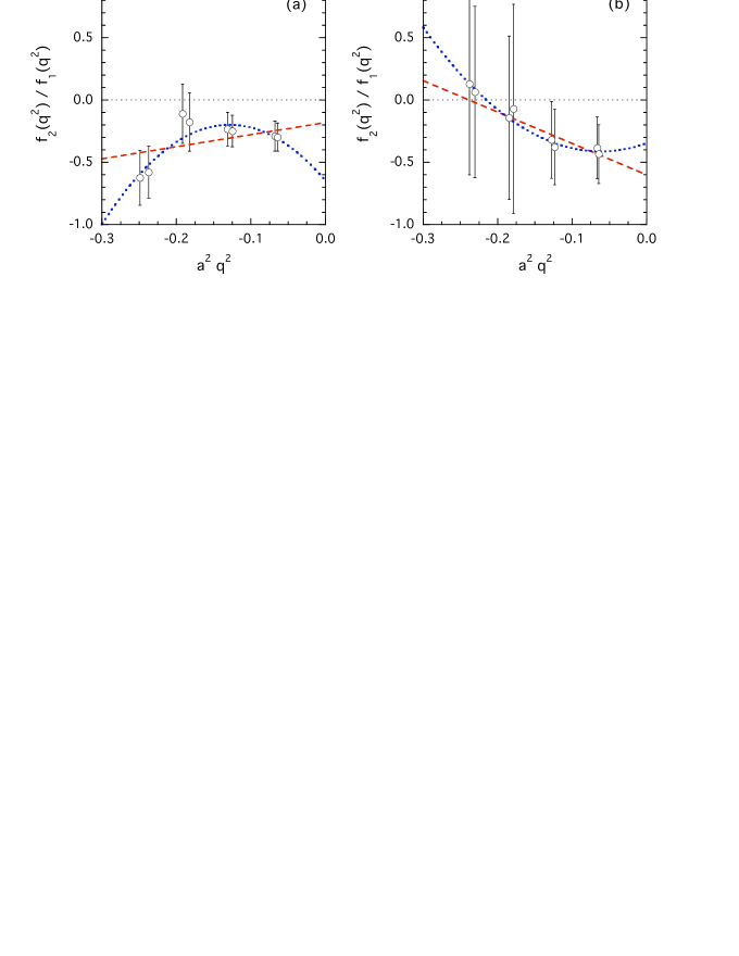
Fig. 10: Values of $f_{2}(q^{2})/f_{1}(q^{2})$ versus $a^{2}q^{2}$ for the two combinations of the hopping parameters $(k_{s},k_{\ell})=(0.1336,0.1340)$ (a) and $(k_{s},k_{\ell})=(0.1345,0.1343)$ (b). The dashed and dotted lines represent linear and quadratic fits in $q^{2}$, respectively.

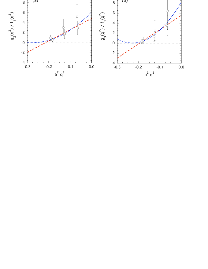
Fig. 11: The same as in Fig. 10 but for the ratio $g_{3}(q^{2})/f_{1}(q^{2})$.

The absence of a determination sufficiently close to $q^{2}=0$ as well as the limited number of points introduces some sensitivity of the values extrapolated at zero-momentum transfer to the specific functional form assumed for the $q^{2}$-dependence of the f.f.’s. The values of the ratios extrapolated to zero-momentum transfer adopting a linear fit in $q^{2}$ are collected in Table 6 and shown in Fig. 12. Note that the uncertainties are always larger than $50\%$.

$k_{s}-k_{\ell}$	$f_{2}(0)/f_{1}(0)$	$g_{3}(0)/f_{1}(0)$
$0.1336-0.1340$	$-0.18~{}(20)$	$4.9~{}(2.7)$
$0.1336-0.1343$	$-0.20~{}(21)$	$4.5~{}(2.7)$
$0.1336-0.1345$	$-0.21~{}(22)$	$3.9~{}(2.6)$
$0.1340-0.1336$	$-0.31~{}(26)$	$5.6~{}(2.9)$
$0.1340-0.1343$	$-0.34~{}(30)$	$4.8~{}(3.1)$
$0.1340-0.1345$	$-0.36~{}(31)$	$4.3~{}(2.9)$
$0.1343-0.1336$	$-0.44~{}(31)$	$5.9~{}(3.2)$
$0.1343-0.1340$	$-0.46~{}(34)$	$5.7~{}(3.4)$
$0.1343-0.1345$	$-0.50~{}(37)$	$5.0~{}(3.5)$
$0.1345-0.1336$	$-0.56~{}(34)$	$6.0~{}(3.4)$
$0.1345-0.1340$	$-0.58~{}(37)$	$5.8~{}(3.6)$
$0.1345-0.1343$	$-0.60~{}(39)$	$5.5~{}(3.8)$

Table 6: Values of the ratios $f_{2}(0)/f_{1}(0)$ and $g_{3}(0)/f_{1}(0)$, obtained by performing a linear fit in $q^{2}$.

The mass dependence of $f_{2}(0)/f_{1}(0)$ is well described by a simple linear fit in $a^{2}(M_{K}^{2}+M_{\pi}^{2})$, whereas the dependence upon the variable $a^{2}(M_{K}^{2}-M_{\pi}^{2})$ is found to be negligible. In the case of $g_{3}(0)/f_{1}(0)$ the findings are opposite and the dependence upon the variable $a^{2}(M_{K}^{2}+M_{\pi}^{2})$ is negligible. Using linear fits in $a^{2}(M_{K}^{2}+M_{\pi}^{2})$ for $f_{2}(0)/f_{1}(0)$ and in $a^{2}(M_{K}^{2}-M_{\pi}^{2})$ for $g_{3}(0)/f_{1}(0)$, we obtain at the physical point: $f_{2}(0)/f_{1}(0)=-1.14\pm 0.66$ and $g_{3}(0)/f_{1}(0)=6.3\pm 3.5$. In order to investigate the stability of the extrapolation we consider also a quadratic fit in $a^{2}(M_{K}^{2}+M_{\pi}^{2})$ for $f_{2}(0)/f_{1}(0)$ and in $a^{2}(M_{K}^{2}-M_{\pi}^{2})$ for $g_{3}(0)/f_{1}(0)$, obtaining the following results that we quote as our final estimates of these quantities

$$\left[\frac{f_{2}(0)}{f_{1}(0)}\right]^{phys.} = -1.52\pm 0.81~{},$$ (44)

$$\left[\frac{g_{3}(0)}{f_{1}(0)}\right]^{phys.} = +6.1\pm 3.3~{}.$$ (45)

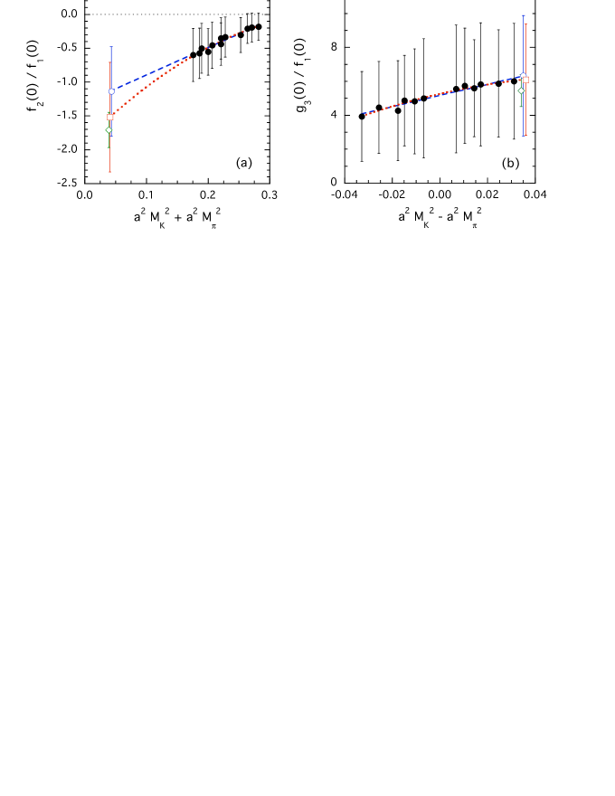
Fig. 12: Results for the ratios $f_{2}(0)/f_{1}(0)$ (a) and $g_{3}(0)/f_{1}(0)$ (b) vs. the meson mass combinations $a^{2}(M_{K}^{2}+M_{\pi}^{2})$ in (a) and $a^{2}(M_{K}^{2}-M_{\pi}^{2})$ in (b), obtained after extrapolation to $q^{2}=0$ through linear fits in $q^{2}$. The dashed (dotted) lines are linear (quadratic) fits and the open dots (squares) are the corresponding values extrapolated to the physical point. The diamond represents: in (a) the experimental value of $f_{2}(0)/f_{1}(0)$ from Ref. [10], and in (b) the value of $g_{3}(0)/f_{1}(0)$, obtained using the generalized Goldberger-Treiman relation [12] and the axial Ward Identity (see text).

In the case of the weak magnetism f.f. the experimental result for $f_{2}(0)/f_{1}(0)$ is known from Ref. [10], namely $f_{2}(0)/f_{1}(0)=-1.71\pm 0.12_{\rm stat.}\pm 0.23_{\rm syst.}$, which is shown in Fig. 12(a). In the case of $g_{3}(0)/f_{1}(0)$ instead there is no direct experimental information. By combining the generalized Goldberger-Trieman relation [12] and the axial Ward identity one can argue that the f.f. $g_{3}(q^{2})$ should have a $K$-meson pole at low values of $q^{2}$, which implies that close to the chiral limit one has

$$\frac{g_{3}(0)}{f_{1}(0)}=\left(\frac{M_{\Sigma}+M_{n}}{M_{K}}\right)^{2}\frac{g_{1}(0)}{f_{1}(0)}~{}.$$ (46)

Using the result (40) we get $g_{3}(0)/f_{1}(0)=5.5\pm 0.9$, which is consistent with Eq. (44). This estimate is also presented in Fig. 12(b). Note that both the latter and the experimental value for $f_{2}(0)/f_{1}(0)$ are quite closer to the results (45) and (44), respectively.

A calculation of the weak magnetism $f_{2}$ and the induced pseudoscalar $g_{3}$ f.f.’s for values of $q^{2}$ closer to $q^{2}=0$ and at lower values of the quark masses is mandatory to improve the precision of the lattice determination of these f.f.’s.

Results for $g_{2}(0)/f_{1}(0)$ and $f_{3}(0)/f_{1}(0)$

The momentum dependence of the ratios $g_{2}(q^{2})/f_{1}(q^{2})$ and $f_{3}(q^{2})/f_{1}(q^{2})$ is presented in Figs. 13 and 14, respectively. In the SU(3) limit both the weak electricity $g_{2}(q^{2})$ and the induced scalar $f_{3}(q^{2})$ f.f.’s vanish identically, so that the results shown in Figs. 13 and 14 are totally generated by the breaking of the SU(3) symmetry. As in the case of $g_{3}(q^{2})/f_{1}(q^{2})$ the statistical error for $g_{2}(q^{2})/f_{1}(q^{2})$ becomes very large for the largest absolute $q^{2}$ value, which therefore is not presented in Fig. 13. Note that in Figs. 13 and 14 we have explicitly reversed the signs of the values of $g_{2}(q^{2})$ and $f_{3}(q^{2})$ corresponding to the $n\rightarrow\Sigma$ transitions, because both $g_{2}(q^{2})$ and $f_{3}(q^{2})$ belong to second-class currents.

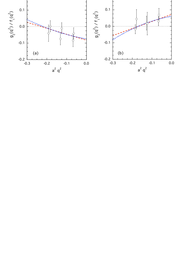
Fig. 13: Values of $g_{2}(q^{2})/f_{1}(q^{2})$ versus $a^{2}q^{2}$ for the two combinations of the hopping parameters $(k_{s},k_{\ell})=(0.1336,0.1340)$ (a) and $(k_{s},k_{\ell})=(0.1345,0.1343)$ (b). The dashed and dotted lines represent linear and quadratic fits in $q^{2}$, respectively.

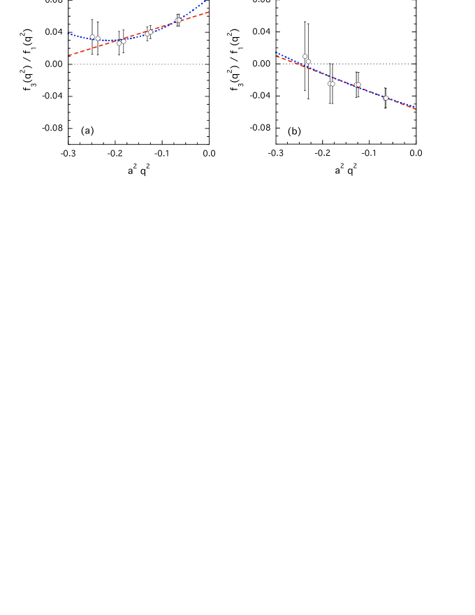
Fig. 14: The same as in Fig. 13 but for the ratio $f_{3}(q^{2})/f_{1}(q^{2})$.

The sensitivity of the extrapolated values at zero-momentum transfer to the specific functional form assumed for the $q^{2}$-dependence of the two ratios $g_{2}(q^{2})/f_{1}(q^{2})$ and $f_{3}(q^{2})/f_{1}(q^{2})$ is much more limited with respect to what has been observed in the case of the ratios $f_{2}(q^{2})/f_{1}(q^{2})$ and $g_{3}(q^{2})/f_{1}(q^{2})$. The values of $g_{2}(0)/f_{1}(0)$ and $f_{3}(0)/f_{1}(0)$, obtained adopting a linear fit in $q^{2}$, are presented in Table 7 and in Figs. 15(a) and 16(a). Note again that, as expected for second-class currents, the signs of both $g_{2}(0)/f_{1}(0)$ and $f_{3}(0)/f_{1}(0)$ are linked to the sign of $a^{2}(M_{K}^{2}-M_{\pi}^{2}$).

$k_{s}-k_{\ell}$	$g_{2}(0)/f_{1}(0)$	$f_{3}(0)/f_{1}(0)$
$0.1336-0.1340$	$-0.083~{}~{}(38)$	$+0.065~{}(14)$
$0.1336-0.1343$	$-0.139~{}~{}(70)$	$+0.123~{}(28)$
$0.1336-0.1345$	$-0.185~{}~{}(92)$	$+0.166~{}(40)$
$0.1340-0.1336$	$+0.100~{}~{}(43)$	$-0.071~{}(19)$
$0.1340-0.1343$	$-0.085~{}~{}(37)$	$+0.064~{}(19)$
$0.1340-0.1345$	$-0.132~{}~{}(66)$	$+0.112~{}(35)$
$0.1343-0.1336$	$+0.220~{}~{}(88)$	$-0.146~{}(47)$
$0.1343-0.1340$	$+0.094~{}~{}(42)$	$-0.070~{}(25)$
$0.1343-0.1345$	$-0.071~{}~{}(32)$	$+0.053~{}(22)$
$0.1345-0.1336$	$+0.326~{}(123)$	$-0.213~{}(80)$
$0.1345-0.1340$	$+0.180~{}~{}(77)$	$-0.132~{}(56)$
$0.1345-0.1343$	$+0.066~{}~{}(33)$	$-0.057~{}(27)$

Table 7: Values of the ratios $g_{2}(0)/f_{1}(0)$ and $f_{3}(0)/f_{1}(0)$, obtained by performing a linear fit in $q^{2}$.

Since the values of $g_{2}(0)/f_{1}(0)$ and $f_{3}(0)/f_{1}(0)$ are exactly known in the SU(3) limit (i.e., $g_{2}(0)/f_{1}(0)=f_{3}(0)/f_{1}(0)=0$), the analysis of the mass dependence of these ratios can proceed in a way similar to the one adopted for $f_{1}(0)$. In this case, however, taking into account that both $g_{2}$ and $f_{3}$ are not protected by the AG theorem, we introduce the following ratios:

$$R_{g_{2}}(M_{K},M_{\pi})=\frac{g_{2}(0)}{f_{1}(0)}\frac{1}{a^{2}(M_{K}^{2}-M_{\pi}^{2})}~{},$$ (47)

$$R_{f_{3}}(M_{K},M_{\pi})=\frac{f_{3}(0)}{f_{1}(0)}\frac{1}{a^{2}(M_{K}^{2}-M_{\pi}^{2})}~{}.$$ (48)

The mass dependence of these quantities is well described by simple linear fits in the mass combination $a^{2}(M_{K}^{2}+M_{\pi}^{2})$, whereas the dependence upon the other variable $a^{2}(M_{K}^{2}-M_{\pi}^{2})$ turns out to be negligible. At the physical point we get $R_{g_{2}}(M_{K}^{phys.},M_{\pi}^{phys.})=18.0\pm 7.5$ and $R_{f_{3}}(M_{K}^{phys.},M_{\pi}^{phys.})=-11.9\pm 6.2$. A quadratic fit in the mass combination $a^{2}(M_{K}^{2}+M_{\pi}^{2})$ does not modify the central value of $R_{g_{2}}$, but it increases the uncertainty, i.e. $R_{g_{2}}(M_{K}^{phys.},M_{\pi}^{phys.})=18.3\pm 14.6$. A slight shift in the central value within a much larger uncertainty is found in the case of $R_{f_{3}}$, namely $R_{f_{3}}(M_{K}^{phys.},M_{\pi}^{phys.})=-18.4\pm 15.5$. Thus, using the values of $R_{g_{2}}$ and $R_{f_{3}}$ from the linear fits, we derive our final estimates of $g_{2}(0)/f_{1}(0)$ and $f_{3}(0)/f_{1}(0)$ extrapolated to the physical point

$$\left[\frac{g_{2}(0)}{f_{1}(0)}\right]^{phys.} = +0.63\pm 0.26~{},$$ (49)

$$\left[\frac{f_{3}(0)}{f_{1}(0)}\right]^{phys.} = -0.42\pm 0.22~{}.$$ (50)

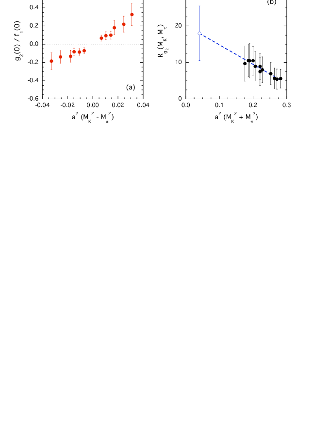
Fig. 15: Results for the ratios $g_{2}(0)/f_{1}(0)$ (a) and $R_{g_{2}}$ (b) vs. the meson mass combinations $a^{2}(M_{K}^{2}-M_{\pi}^{2})$ in (a) and $a^{2}(M_{K}^{2}+M_{\pi}^{2})$ in (b), obtained after extrapolation to $q^{2}=0$ through linear fits in $q^{2}$. The dashed line is the result of a linear fit and the open dot is the corresponding value extrapolated to the physical point.

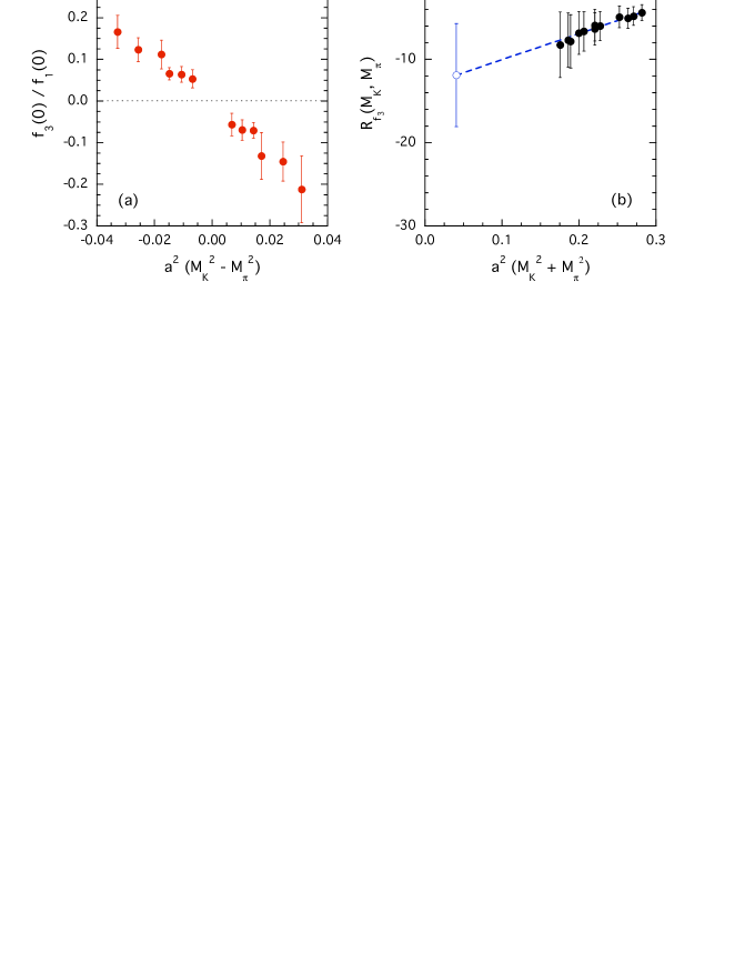
Fig. 16: The same as in Fig. 15 but for the ratios $f_{3}(0)/f_{1}(0)$ (a) and $R_{f_{3}}$ (b).

Our results indicate a positive, non-vanishing value of $g_{2}(0)/f_{1}(0)$ due to SU(3)-breaking corrections. In the experiments neither $g_{1}(0)/f_{1}(0)$ nor $g_{2}(0)/f_{1}(0)$ are separately determined, but only a specific combination of these ratios can be extracted. The following combination has been determined for the $\Sigma^{-}\rightarrow n$ transition [10]

$$\left|\frac{g_{1}(0)-0.133\cdot g_{2}(0)}{f_{1}(0)}\right|^{exp.}=0.327\pm 0.007_{\rm stat.}\pm 0.019_{\rm syst.}~{}.$$ (51)

Using our results (40) and (49) we get

$$\left|\frac{g_{1}(0)-0.133\cdot g_{2}(0)}{f_{1}(0)}\right|^{phys.}=0.37\pm 0.08~{}$$ (52)

in good agreement with the experimental value. Even though the experimental data are compatible with general fitting procedures which make the conventional assumption $g_{2}(q^{2})=0$ (as done for instance in Ref. [3]), it has been found that positive values for $g_{2}(0)/f_{1}(0)$ combined with a corresponding reduced value for $|g_{1}(0)/f_{1}(0)|$ are slightly preferred [10]. The lattice results (40) and (49) appear to favor the second scenario.

7 Conclusions

We have presented a lattice QCD study of SU(3)-breaking corrections in the vector and axial form factors relevant for the hyperon semileptonic decay $\Sigma^{-}\rightarrow n~{}\ell~{}\nu$. Though our simulation has been carried out in the quenched approximation, our results represent the first attempt to evaluate hyperon form factors using a non-perturbative method based only on QCD.

For each form factor we have studied its momentum and mass dependencies, obtaining its value extrapolated at zero-momentum transfer and at the physical point. Our final results are collected in Table 8, where the errors do not include the quenching effect.

$f_{1}(0)$	$-0.988\pm 0.029_{\rm lattice}\pm 0.040_{\rm HBChPT}$
$g_{1}(0)/f_{1}(0)$	$-0.287\pm 0.052$
$f_{2}(0)/f_{1}(0)$	$-1.52\pm 0.81$
$f_{3}(0)/f_{1}(0)$	$-0.42\pm 0.22$
$g_{2}(0)/f_{1}(0)$	$+0.63\pm 0.26$
$g_{3}(0)/f_{1}(0)$	$+6.1\pm 3.3$

Table 8: Results of our lattice calculations of the vector and axial form factors for the $\Sigma^{-}\rightarrow n$ transition.

We conclude with few additional comments:

• The SU(3)-breaking corrections to the vector form factor at zero-momentum transfer, $f_{1}(0)$, have been determined with great statistical accuracy in the regime of the simulated quark masses, which correspond to pion masses above $0.7$ GeV. The magnitude of the errors reported in Table 8 is mainly due to the chiral extrapolation and to the poor convergence of the Heavy Baryon Chiral Perturbation Theory [7]. Though within large errors the central value of $f_{1}(0)$ arises from a partial cancellation between the contributions of local terms, evaluated on the lattice, and chiral loops. This may indicate that SU(3)-breaking corrections on $f_{1}(0)$ are moderate (at least for the transition considered), giving support to the analysis of Ref. [3].

• The ratio $g_{1}(0)/f_{1}(0)$ is found to be negative and consistent with the value adopted in the analysis of Ref. [3]. The study of the degenerate transitions also allowed us to determine the value of $g_{1}(0)/f_{1}(0)$ directly in the limit of exact SU(3) symmetry, obtaining $[g_{1}(0)/f_{1}(0)]_{SU(3)}=-0.269\pm 0.047$. This means that SU(3)-breaking corrections are moderate also on this ratio, though the latter is not protected by the Ademollo-Gatto theorem against fist-order corrections.

• The weak electricity form factor at zero-momentum transfer $g_{2}(0)$ is found to be non-vanishing because of SU(3)-breaking corrections. Our result for $g_{1}(0)/f_{1}(0)$ combined with that of $g_{2}(0)/f_{1}(0)$ are nicely consistent with the experimental result from [10]. Our findings favor the scenario in which $g_{2}(0)/f_{1}(0)$ is large and positive with a corresponding reduced value for $|g_{1}(0)/f_{1}(0)|$ with respect to the conventional assumption $g_{2}(q^{2})=0$ (done for instance in Ref. [3]) based on exact SU(3) symmetry.

Finally, we discuss few possible improvements for future lattice QCD studies of the hyperon semileptonic transitions:

• The quenched approximation should be removed and the simulated quark masses should be lowered as much as possible in order to reduce the impact of the chiral extrapolation.

• The accuracy of the ratios $f_{2}(0)/f_{1}(0)$, $f_{3}(0)/f_{1}(0)$, $g_{2}(0)/f_{1}(0)$ and $g_{3}(0)/f_{1}(0)$ can be improved by implementing twisted boundary conditions for the quark fields. In this way values of the momentum transfer closer to $q^{2}=0$ can be accessed in the simulations.

• The use of smeared source and sink for the interpolating fields as well as the use of several, independent interpolating fields may help in increasing the overlap with the ground-state signal, particularly at low values of the quark masses.

References

- [1] D. Becirevic et al., “The K pi vector form factor at zero momentum transfer on the lattice”, Nucl. Phys. B 705 (2005) 339 [arXiv:hep-ph/0403217]; Eur. Phys. J. A 24S1 (2005) 69 [arXiv:hep-lat/0411016].
- [2] C. Dawson, T. Izubuchi, T. Kaneko, S. Sasaki and A. Soni, “Vector form factor in K(l3) semileptonic decay with two flavors of dynamical domain-wall quarks”, [arXiv:hep-ph/0607162]. N. Tsutsui et al. [JLQCD Collaboration], “Kaon semileptonic decay form factors in two-flavor QCD”, PoS LAT2005 (2005) 357 [arXiv:hep-lat/0510068]. M. Okamoto [Fermilab Lattice, MILC and HPQCD Collaborations], “Semileptonic decays of D, B, K mesons and the full CKM matrix from unquenched lattice QCD”, Int. J. Mod. Phys. A 20 (2005) 3469. See also: M. Okamoto, “Full determination of the CKM matrix using recent results from lattice QCD”, PoS LAT2005 (2006) 013 [arXiv:hep-lat/0510113].
- [3] N. Cabibbo, E. C. Swallow and R. Winston, “Semileptonic hyperon decays and CKM unitarity”, Phys. Rev. Lett. 92 (2004) 251803 [arXiv:hep-ph/0307214]; Ann. Rev. Nucl. Part. Sci. 53 (2003) 39 [arXiv:hep-ph/0307298].
- [4] M. Ademollo and R. Gatto, “Nonrenormalization theorem for the strangeness violating vector currents”, Phys. Rev. Lett. 13 (1964) 264.
- [5] V. Mateu and A. Pich, “V(us) determination from hyperon semileptonic decays”, JHEP 0510 (2005) 041 [arXiv:hep-ph/0509045].
- [6] D. Guadagnoli, G. Martinelli, M. Papinutto and S. Simula, “Semileptonic hyperon decays on the lattice: An exploratory study”, Nucl. Phys. Proc. Suppl. 140 (2005) 390 [arXiv:hep-lat/0409048]. D. Guadagnoli, V. Lubicz, G. Martinelli, M. Papinutto, S. Simula and G. Villadoro, “Chiral extrapolation of hyperon vector form factors”, PoS LAT2005 (2005) 358 [arXiv:hep-lat/0509061].
- [7] G. Villadoro, “Chiral corrections to the hyperon vector form factors”, Phys. Rev. D 74 (2006) 014018 [arXiv:hep-ph/0603226].
- [8] K. Sasaki and S. Sasaki, “Excited baryon spectroscopy from lattice QCD: Finite size effect and hyperfine mass splitting”, Phys. Rev. D 72 (2005) 034502 [arXiv:hep-lat/0503026]. R. G. Edwards et al. [LHPC Collaboration], “The nucleon axial charge in full lattice QCD”, Phys. Rev. Lett. 96 (2006) 052001 [arXiv:hep-lat/0510062]. A. A. Khan et al. [QCDSF Collaboration], “Axial coupling constant of the nucleon for two flavours of dynamical quarks in finite and infinite volume”, [arXiv:hep-lat/0603028].
- [9] N. Cabibbo, “Unitary Symmetry And Leptonic Decays”, Phys. Rev. Lett. 10 (1963) 531.
- [10] S. Y. Hsueh et al., “A high precision measurement of polarized sigma- beta decay”, Phys. Rev. D 38 (1988) 2056.
- [11] A. Sirlin, Nucl. Phys. B 161 (1979) 301.
- [12] M. Goldberger and S.B. Treiman, Phys. Rev. 110 (1958) 1178; ibid. 110 (1958) 1478; ibid. 111 (1958) 354.
- [13] M. Luscher, S. Sint, R. Sommer and H. Wittig, “Non-perturbative determination of the axial current normalization constant in O(a) improved lattice QCD”, Nucl. Phys. B 491 (1997) 344 [arXiv:hep-lat/9611015]. T. Bhattacharya, R. Gupta, W. J. Lee and S. R. Sharpe, “Order a improved renormalization constants”, Phys. Rev. D 63 (2001) 074505 [arXiv:hep-lat/0009038]; “Scaling behavior of improvement and renormalization constants”, Nucl. Phys. Proc. Suppl. 106, 789 (2002) [arXiv:hep-lat/0111001].
- [14] M. Luscher, S. Sint, R. Sommer, P. Weisz and U. Wolff, “Non-perturbative O(a) improvement of lattice QCD”, Nucl. Phys. B 491 (1997) 323 [arXiv:hep-lat/9609035].
- [15] S. Hashimoto et al., “Lattice QCD calculation of anti-B D l anti-nu decay form factors at zero recoil”, Phys. Rev. D 61 (2000) 014502 [arXiv:hep-ph/9906376].
- [16] P. Mergell, U. G. Meissner and D. Drechsel, “Dispersion theoretical analysis of the nucleon electromagnetic form-factors”, Nucl. Phys. A 596 (1996) 367 [arXiv:hep-ph/9506375]. H. W. Hammer, U. G. Meissner and D. Drechsel, “Dispersion-theoretical analysis of the nucleon electromagnetic form factors: Inclusion of time-like data”, Phys. Lett. B 385 (1996) 343 [arXiv:hep-ph/9604294].
- [17] D. Guadagnoli, M. Papinutto and S. Simula, “Extracting excited states from lattice QCD: The Roper resonance”, Phys. Lett. B 604 (2004) 74 [arXiv:hep-lat/0409011]; Nucl. Phys. A 755 (2005) 485.
- [18] A. Krause, “Baryon Matrix Elements Of The Vector Current In Chiral Perturbation Theory”, Helv. Phys. Acta 63 (1990) 3.
- [19] J. Anderson and M. A. Luty, “Chiral corrections to hyperon vector form-factors”, Phys. Rev. D 47 (1993) 4975.
- [20] E. Jenkins and A. V. Manohar, “Chiral corrections to the baryon axial currents”, Phys. Lett. B 259 (1991) 353.
- [21] T. R. Hemmert, B. R. Holstein and J. Kambor, “Chiral Lagrangians and Delta(1232) interactions: Formalism”, J. Phys. G 24 (1998) 1831 [arXiv:hep-ph/9712496].
- [22] E. Jenkins and A. V. Manohar, “Baryon Chiral Perturbation Theory Using A Heavy Fermion Lagrangian”, Phys. Lett. B 255 (1991) 558.
- [23] J.M. Gaillard and G. Sauvage, Ann. Rev. Nucl. Part. Sci. 34, 351 (1984).
- [24] P. F. Bedaque, “Aharonov-Bohm effect and nucleon nucleon phase shifts on the lattice”, Phys. Lett. B 593 (2004) 82 [arXiv:nucl-th/0402051]. G. M. de Divitiis, R. Petronzio and N. Tantalo, “On the discretization of physical momenta in lattice QCD”, Phys. Lett. B 595 (2004) 408 [arXiv:hep-lat/0405002]. C. T. Sachrajda and G. Villadoro, “Twisted boundary conditions in lattice simulations”, Phys. Lett. B 609 (2005) 73 [arXiv:hep-lat/0411033]. J. M. Flynn, A. Juttner and C. T. Sachrajda [UKQCD Collaboration], “A numerical study of partially twisted boundary conditions”, Phys. Lett. B 632 (2006) 313 [arXiv:hep-lat/0506016].
- [25] D. Guadagnoli, F. Mescia and S. Simula, “Lattice study of semileptonic form factors with twisted boundary conditions”, Phys. Rev. D 73 (2006) 114504 [arXiv:hep-lat/0512020].
- [26] S. Weinberg, “Charge symmetry of weak interactions”, Phys. Rev. 112 (1958) 1375.