ROMA-1431/06

TU-772

Bulk Mass Effects in Gauge-Higgs Unification
at Finite Temperature

Nobuhito Maru^(a) , Kazunori Takenaga^(b)

^(a) Dipartimento di Fisica, Università di Roma ”La Sapienza”
and INFN, Sezione di Roma, P.le Aldo Moro, I-00185 Roma, Italy

^(b) Department of Physics, Tohoku University, Sendai 980-8578, Japan

We study the bulk mass effects on the electroweak phase transition at finite temperature in a five dimensional $SU(3)$ gauge-Higgs unification model on an orbifold. We investigate whether the Higgs mass satisfying the experimental lower bound can be compatible with the strong first order phase transition necessary for a successful electroweak baryogenesis. Our numerical results show that the above statement can be realized by matter with bulk mass yielding a viable Higgs mass. We also find an interesting case where the heavier Higgs gives the stronger first order phase transition.

1 Introduction

Solving the gauge hierarchy problem is one of the guidelines to consider the physics beyond the Standard Model. Low energy supersymmetry is well motivated theory to solve the gauge hierarchy problem. Furthermore, it predicts the gauge coupling unification and the natural candidate for the dark matter. However, the superparticle has not yet been discovered so far. Therefore, it is worth while to explore other possibilities beyond the Standard Model. Recent developments of the physics of extra dimensions offer many new insights into the four dimensional physics including the gauge hierarchy problem.

The gauge-Higgs unification [1]-[4] is one of the attractive scenarios of this kind. In this scenario, the Higgs scalar is originated from the extra component of the gauge field in higher dimensions and the gauge symmetry breaking occurs by the vacuum expectation value (VEV) through the dynamics of the Wilson line phases called as Hosotani mechanism [5]. Now, the gauge-Higgs unification has been widely studied from the various viewpoints [6]-[15].

Remarkable thing is that the Higgs mass at the classical level is forbidden by the higher dimensional gauge symmetry. Furthermore, the Higgs mass is generated by quantum corrections and insensitive to the cutoff scale. This is an essential feature of solving the gauge hierarchy problem. In fact, explicit calculations showing the finiteness of the Higgs mass are known for the five dimensional(5D) QED compactified on $S^{1}$ at one-loop level [3] and two-loop level[14], 5D non-Abelian gauge theory on an orbifold $S^{1}/Z_{2}$ at one-loop level [16], and 6D $U(3)\times U(3)$ gauge theory on toroidal compactification at one-loop level [4] [17], and 6D massive scalar QED on $S^{2}$ at one-loop level [15]. Even in the Gravity-Gauge-Higgs unification scenario, the Higgs mass is shown to be finite at one-loop level in 5D gravity theory on $S^{1}$coupled to the bulk scalar field [18].

However, it is highly nontrivial task to obtain the phenomenologically viable Higgs mass in such a scenario because the Higgs quartic coupling is also generated at one-loop level, which implies that the Higgs mass is generically too small. Recent works for this problem are found in [7] in terms of large representation fermion contributions and [8] in terms of the explicit 5D Lorentz symmetry breaking effects. In our previous paper [13], we have proposed another solution of this problem. We have investigated the bulk mass effects on the electroweak symmetry breaking and the size of Higgs mass. The bulk mass of matter fields is a necessary ingredient in gauge-Higgs unification to discuss Yukawa hierarchy [19] and the pattern of the gauge symmetry breaking [10]. We have found some simple matter content satisfying the lower bound of Higgs mass where the fields with an antiperiodic boundary condition play an important role to make the Higgs VEV small.

On the other hand, one of the interesting applications of gauge-Higgs unification is the electroweak baryogenesis at finite temperature [11, 12]. The dynamics of Wilson line phases is essentially the Coleman-Weinberg mechanism [20], so that the phase transition at finite temperature is expected to be the first order [21]. As will be discussed later, the first order phase transition is controlled by the cubic term of the effective potential, which originates from the zero mode of bosonic fields. Comparing to the four dimensional case, the contributions from the higher dimensional gauge field is crucial to strengthen the first order phase transition.

In [12], we have studied the finite temperature behavior of the 5D $SU(3)$ gauge-Higgs unification models with massless bulk matter in adjoint and the fundamental representations. In fact, we have confirmed that the phase transition is indeed the first order and found some examples of matter content satisfying the Higgs mass lower bound and the strong first order transition necessary for the baryogenesis. As stated above, since the bulk mass is indispensable in gauge-Higgs unification, it is worth while to study the bulk mass effects on the electroweak phase transition at finite temperature.

From these motivations, in this paper, we investigate the gauge-Higgs unification with massive bulk matter at finite temperature and focus on the possibility that the Higgs mass satisfying the experimental lower bound and the strong first order phase transition required for successful electroweak baryogenesis are compatible. Due to the general properties that the large dimensional representation fermions weaken the first phase transition [22], we consider the bulk matter with only the fundamental and the adjoint representations as in [12]. We find that the matter content considered in [13] have a strong first order phase transition enough for a successful electroweak baryogenesis. And we also find an interesting case where the heavier Higgs mass has the stronger first order phase transition.

This paper is organized as follows. In the next section, we derive the one-loop effective potential at finite temperature for the Higgs field. The results obtained in [13] for the analysis of the Higgs mass is reviewed. Section 3 is the main part of this paper, where the bulk mass effects on the electroweak phase transition at finite temperature is investigated using the models studied in [13]. Section 4 is devoted to the conclusions of this paper.

2 Effective potential of the model

Let us study the effect of the finite temperature on the gauge-Higgs unification. Namely, we are interested in the order of the phase transition caused by the dynamics of the Wilson line (Hosotani mechanism). We take the $D$ dimensional space-time to be

$$M^{D}=(S^{1}\times R^{D-2})\times S^{1}/Z_{2},$$ (2.1)

where one of the spatial coordinate is compactified on an orbifold, $S^{1}/Z_{2}$ and the Euclidean time direction corresponds to a circle $S^{1}$. Accordingly, the gauge potential is decomposed as

$$A_{\hat{\mu}}\equiv A_{\hat{\mu}}^{a}T^{a}=(A_{0},A_{i},A_{y})\qquad(i=1,\cdots,D-2),$$ (2.2)

where $T^{a}$ is the generators of the gauge group we are considering with the normalization being $\mbox{tr}(T^{a}T^{b})={1\over 2}\delta_{ab}$.

We consider the $SU(3)$ gauge group as the simplest example of the gauge-Higgs unification. One of the spatial coordinate is an $S^{1}/Z_{2}$, so that there are two fixed points at $y=0,\pi R$, where $R$ is the radius of $S^{1}$. Considering the gauge theory on such a space-time, one needs to specify the boundary conditions of fields for the $S^{1}$ direction and the fixed point. Here we define them as

$$A_{\hat{\mu}}(x,y+2\pi R) = UA_{\hat{\mu}}(x,y)\,U^{\dagger},$$ (2.3)

$$\pmatrix{A_{\mu}\cr A_{y}\cr}(x,y_{i}-y) = P_{i}\pmatrix{A_{\mu}\cr-A_{y}\cr}(x,y_{i}+y)\,P_{i}^{\dagger},~{}~{}(i=0,1)$$ (2.4)

where $U^{\dagger}=U^{-1},P_{i}^{\dagger}=P_{i}=P_{i}^{-1}$ and $y_{0}=0,y_{1}=\pi R$. The minus sign for $A_{y}$ is needed to preserve the gauge invariance under these transformations. Since a transformation $\pi R+y\rightarrow\pi R-y$ must be the same as a transformation $\pi R+y\rightarrow-(\pi R+y)\rightarrow\pi R-y$, we obtain

$$U=P_{1}P_{0}.$$ (2.5)

Hereafter, we consider $P_{i}$ to be fundamental quantities.

The gauge symmetry at low energies is determined by counting the zero modes associated with $A_{\mu}$ for each $P_{0,1}$ at the tree level. We are interested in how the electroweak gauge symmetry, $SU(2)\times U(1)$ is broken at the quantum level. Therefore, we break the original $SU(3)$ gauge symmetry by the orbifolding down to $SU(2)\times U(1)$ by taking $P_{0}=P_{1}=\mbox{diag}(-1,-1,1)$. Then, the zero mode are found to be

$$A_{\mu}^{(0)} = {1\over 2}\pmatrix{A_{\mu}^{3}+{A_{\mu}^{8}\over\sqrt{3}}&A_{\mu}^{1}-iA_{\mu}^{2}&0\cr A_{\mu}^{1}+iA_{\mu}^{2}&-A_{\mu}^{3}+{A_{\mu}^{8}\over\sqrt{3}}&0\cr 0&0&-{2\over\sqrt{3}}A_{\mu}^{8}},$$ (2.6)

$$A_{y}^{(0)} = {1\over 2}\pmatrix{0&0&A_{y}^{4}-iA_{y}^{5}\cr 0&0&A_{y}^{6}-iA_{y}^{7}\cr A_{y}^{4}+iA_{y}^{5}&A_{y}^{6}+iA_{y}^{7}&0}.$$ (2.7)

One can observe that the zero mode of $A_{y}$

$$\Phi\equiv\pmatrix{A_{y}^{4}-iA_{y}^{5}\cr A_{y}^{6}-iA_{y}^{7}\cr}$$ (2.8)

transforms as a doublet under the $SU(2)$ gauge symmetry, so that we can regard $\Phi$ as the Higgs doublet in the Standard Model.

By using the $SU(2)\times U(1)$ degrees of freedom, the VEV of $A_{y}$ $(\langle A_{y}\rangle)$ can be parameterized as

$$\langle A_{y}\rangle={a\over{gR}}{\lambda^{6}\over 2},$$ (2.9)

where $\lambda^{6}$ is the sixth Gell-Mann matrix and $a$ is a dimensionless real parameter. $g$ is the five dimensional gauge coupling whose mass dimension is $-1/2$. The parameter $a$ is closely related to the Wilson line phases as follows,

$$W = {\cal P}\mbox{exp}\left(ig\oint_{S^{1}}dyA_{y}\right)=\pmatrix{1&0&0\cr 0&\cos(\pi a)&i\sin(\pi a)\cr 0&i\sin(\pi a)&\cos(\pi a)}\qquad(\mbox{mod}~{}2)$$ (2.12)

$$= \left\{\begin{array}[]{llll}\mbox{diag}(1,1,1)&\mbox{for}&a=0,&SU(2)\times U(1),\\ \mbox{diag}(1,-1,-1)&\mbox{for}&a=1,&U(1)^{\prime}\times U(1).\end{array}\right.$$

We observe that the gauge symmetry breaking patterns are classified by the values of $a$ and in order to obtain the desirable electroweak symmetry breaking $SU(2)\times U(1)\rightarrow U(1)$, one needs the fractional values of $a$. As we will see later, the values of $a$ is determined dynamically through the dynamics of the Wilson line phases.

As mentioned in our previous paper [13], we note that the bulk mass term of fermions in five dimensions is odd under the parity transformation $y\to-y(\pi R+y\to\pi R-y)$. We introduce a pair of fields $\psi_{\pm}$ whose parity is given by $\psi_{\pm}(-y)=\pm\psi_{\pm}(y)$ to obtain the mass term like $M\bar{\psi}_{+}\psi_{-}$ where $M$ is a constant. Let us suppose that $\psi^{(\pm)}$ and ${\tilde{\psi}}^{(\pm)}$ belong to the fundamental representation under the $SU(3)$ gauge group and satisfy the following boundary conditions ,

type I ; $$\left\{\begin{array}[]{l}\psi^{(\pm)}(-y)=\pm P_{0}~{}i\Gamma^{y}~{}\psi^{(\pm)}(y)\\[8.5359pt] \psi^{(\pm)}(\pi R-y)=\pm P_{1}~{}i\Gamma^{y}~{}\psi^{(\pm)}(\pi R+y),\end{array}\right.$$ (2.15)

type II ; $$\left\{\begin{array}[]{l}{\tilde{\psi}}^{(\pm)}(-y)=\pm P_{0}~{}i\Gamma^{y}~{}{\tilde{\psi}}^{(\pm)}(y)\\[8.5359pt] {{\tilde{\psi}}}^{(\pm)}(\pi R-y)=\mp P_{1}~{}i\Gamma^{y}~{}{{\tilde{\psi}}}^{(\pm)}(\pi R+y).\end{array}\right.$$ (2.18)

Equipped with these fields, a pair $(\psi^{(+)},\psi^{(-)})(({\tilde{\psi}}^{(+)},{\tilde{\psi}}^{(-)})$ can have the parity even and gauge invariant bulk mass term, $M{\bar{\psi}}^{(\pm)}\psi^{(\mp)}(M{\bar{\tilde{\psi}}}^{(\pm)}{\tilde{\psi}}^{(\mp)})$. It is easy to see that the field $\psi^{\pm}$ satisfies the periodic boundary condition, $\psi^{\pm}(y+L)=\psi^{\pm}(y)$, while ${\tilde{\psi}}^{\pm}$ does the antiperiodic boundary condition, ${\tilde{\psi}}^{\pm}(y+L)=-{\tilde{\psi}}^{\pm}(y)$.

Let us first calculate the bosonic effective potential at finite temperature for the real parameter $a$. The finite temperature part of the effective potential is taken into account by compactifying the Euclidean time direction on $S^{1}$ with period being $\beta=T^{-1}$, where $T$ is the temperature. And accordingly, the momentum for the time direction is discretized as

$$p_{\tau}=2\pi l\times T,\qquad l\in{\bf Z}.$$ (2.19)

Hence, the effective potential we study is

$$V_{B}^{T}=N_{{\rm deg}}^{\rm B}{T\over{2L}}\sum_{l,n=-\infty}^{\infty}\int{{d^{D-2}p_{E}}\over{(2\pi)^{D-2}}}{\rm ln}\Biggl{[}p_{E(D-2)}^{2}+(2\pi T)^{2}l^{2}+\left({{n+Qa-{\delta\over 2}}\over R}\right)^{2}+M^{2}\Biggr{]},$$ (2.20)

where $N_{{\rm deg}}^{\rm B}$ denotes the on-shell degrees of freedom of the bosonic fields we concern. The charge $Q$ is ${1\over 2}$ for matter belonging to the fundamental representation under the gauge group, and for other representation the expression is given by the combination of Eq. (2.20) with the suitable values of $Q$. And $\delta$ takes $0$ or $1$, depending on the periodicity for the $S^{1}$ direction [13]. In Eq.(2.20), the 4D momentum is taken to be Euclidean. $M$ stands for the bulk mass of the matter fields which was not considered in the previous paper [12].

On the other hand, as for fermions, according to the quantum statistics, since the fermion must take the anti-periodic boundary condition for the Euclidean time direction, contrary to the boson taking the periodic one, we have

$$p_{\tau}=2\pi\left(l+{1\over 2}\right)\times T.$$ (2.21)

Hence, for fermions we study

$$V_{F} = -2^{\left[\frac{D}{2}\right]}(2N^{pair}){T\over{2L}}\sum_{l,n=-\infty}^{\infty}\int{{d^{D-2}p_{E}}\over{(2\pi)^{D-2}}}$$ (2.22)

$$\times {\rm ln}\Biggl{[}p_{E(D-2)}^{2}+(2\pi T)^{2}(l+{1\over 2})^{2}+\left({{n+Qa-{\delta\over 2}}\over R}\right)^{2}+M^{2}\Biggr{]},$$

where it is understood that $\delta$ takes $0$ or $1$.

We can separate the zero temperature $(l=0)$ and the finite temperature parts as $V_{B(F)}=V_{B(F)}^{T=0}+V_{B(F)}^{T\neq 0}$. We regularize the zero temperature part of the effective potential by subtracting the $n=0$ mode. On the other hand, the remaining finite temperature part of the effective potential has no divergence thanks to the Boltzmann suppression factor associated with the finite temperature. Following the usual prescription [22], we obtain the effective potential for bosons

$$V_{B}^{T=0} = -N_{{\rm deg}}^{\rm B}\frac{2}{(2\pi)^{\frac{D}{2}}}\sum_{n=1}^{\infty}\left(\frac{M}{nL}\right)^{\frac{D}{2}}K_{\frac{D}{2}}(nLM)\cos\left[2\pi n\left(Qa-{\delta\over 2}\right)\right],$$ (2.23)

$$V_{B}^{T\neq 0} = -N_{{\rm deg}}^{\rm B}\frac{4}{(2\pi)^{\frac{D}{2}}}\sum_{l=1}^{\infty}\sum_{n=1}^{\infty}\left(\frac{M^{2}T^{2}}{(nLT)^{2}+l^{2}}\right)^{\frac{D}{4}}K_{\frac{D}{2}}\left(\frac{M}{T}\sqrt{(nLT)^{2}+l^{2}}\right)$$ (2.24)

$$\times\cos\left[2\pi n\left(Qa-{\delta\over 2}\right)\right],$$

where $K_{n}(x)$ is the modified Bessel function. Similarly, the fermion contribution to the effective potential at finite temperature is calculated as

$$V_{F} = V_{F}^{T=0}+V_{F}^{T\neq 0}$$

$$= 2^{\left[\frac{D}{2}\right]}(2N^{pair})\frac{2}{(2\pi)^{\frac{D}{2}}}\left[\sum_{n=1}^{\infty}\left(\frac{M}{nL}\right)^{\frac{D}{2}}K_{\frac{D}{2}}(LMn)\right.$$

$$\left.+2\sum_{l=1}^{\infty}\sum_{n=1}^{\infty}(-1)^{l}\left(\frac{M^{2}T^{2}}{(nLT)^{2}+l^{2}}\right)^{\frac{D}{4}}K_{\frac{D}{2}}\left(\frac{M}{T}\sqrt{(nLT)^{2}+l^{2}}\right)\right]\cos\left[2\pi n\left(Qa-{\delta\over 2}\right)\right].$$

2.1 Review of Higgs mass results

In this subsection, we focus on the model of an $SU(3)$ gauge theory in five dimensions introduced in the previous section. For completeness, we briefly review the numerical results of Higgs mass studied in the previous paper [13]. Then, the phase transition at finite temperature will be investigated in the next section using the same models reviewed here.

Following the definition in [13], we introduce the flavor numbers specifying the matter content as

$$(N_{adj}^{I},N_{fd}^{I},N_{adj}^{(+)s},N_{fd}^{(+)s};N_{adj}^{II},N_{fd}^{II},N_{adj}^{(-)s},N_{fd}^{(-)s})$$ (2.26)

where the matter representation under $SU(3)$ gauge group is the adjoint or the fundamental representations. The index $s$ means the scalar field. $I,II$ denote the type of the boundary conditions for fermions defined in (2.15) and (2.18). $(+),(-)$ denotes the $\eta$-parity of the scalar field which is essentially same as the periodic, antiperiodic field, respectively.

Let us consider the following two cases and list up the corresponding results in Table 1 and 2 which were obtained in [13].

$$(\mbox{A})~{}~{}(N_{adj}^{I},N_{fd}^{I},N_{adj}^{(+)s},N_{fd}^{(+)s};N_{adj}^{II},N_{fd}^{II},N_{adj}^{(-)s},N_{fd}^{(-)s}) = (1,1,0,0;1,1,1,0),$$ (2.27)

$$(\mbox{B})~{}~{}(N_{adj}^{I},N_{fd}^{I},N_{adj}^{(+)s},N_{fd}^{(+)s};N_{adj}^{II},N_{fd}^{II},N_{adj}^{(-)s},N_{fd}^{(-)s}) = (1,1,0,2;1,1,2,0).$$ (2.28)

$$\begin{array}[]{|c|cccc|ccccccc|}\hline\cr&z_{adj}^{(+)}&z_{fd}^{(+)}&z_{adj}^{(+)s}&z_{fd}^{(+)s}&z_{adj}^{(-)}&z_{fd}^{(-)}&z_{adj}^{(-)s}&z_{fd}^{(-)s}&{1\over{g_{4}R}}&a_{0}&m_{H}/g_{4}^{2}\\ \hline\cr\hline\cr(1)&0&0&\mbox{-}&\mbox{-}&0&0&0&\mbox{-}&6.3&0.039&134.0\\ \hline\cr(2)&0.1&0.2&\mbox{-}&\mbox{-}&0&0&0&\mbox{-}&12.4&0.020&139.4\\ \hline\cr(3)&0&0&\mbox{-}&\mbox{-}&0&0&0.5&\mbox{-}&7.7&0.032&141.0\\ \hline\cr(4)&0.1&0.2&\mbox{-}&\mbox{-}&0&0&0.2&\mbox{-}&14.0&0.018&140.4\\ \hline\cr(5)&0.1&0.2&\mbox{-}&\mbox{-}&0.1&0&0&\mbox{-}&10.4&0.024&137.2\\ \hline\cr(6)&0.1&0.2&\mbox{-}&\mbox{-}&0&0.2&0&\mbox{-}&11.0&0.022&137.9\\ \hline\cr(7)&0.2&0.2&\mbox{-}&\mbox{-}&0.3&0.3&0&\mbox{-}&24.0&0.010&109.1\\ \hline\cr\end{array}$$

Table 1: Higgs mass results of the matter content (A). The dimensionless parameter $z$ is defined as $z\equiv ML$.

$$\begin{array}[]{|c|cccc|ccccccc|}\hline\cr&z_{adj}^{(+)}&z_{fd}^{(+)}&z_{adj}^{(+)s}&z_{fd}^{(+)s}&z_{adj}^{(-)}&z_{fd}^{(-)}&z_{adj}^{(-)s}&z_{fd}^{(-)s}&{1\over{g_{4}R}}&a_{0}&m_{H}/g_{4}^{2}\\ \hline\cr\hline\cr(1)&0&0&\mbox{-}&0&0&0&0&\mbox{-}&4.0&0.062&117.4\\ \hline\cr(2)&0.2&0.2&\mbox{-}&0.2&0&0&0&\mbox{-}&10.4&0.024&118.6\\ \hline\cr(3)&0.2&0.1&\mbox{-}&0.2&0&0&0&\mbox{-}&7.7&0.032&120.0\\ \hline\cr(4)&0.2&0.25&\mbox{-}&0.2&0&0&0&\mbox{-}&15.5&0.016&115.0\\ \hline\cr(5)&0.2&0.3&\mbox{-}&0.5&0&0&0&\mbox{-}&7.5&0.033&118.2\\ \hline\cr\end{array}$$

Table 2: Higgs mass results of the matter content (B).

We discussed in [13] that the viable Higgs mass is obtained by an interplay of the bulk mass effects between the periodic and the antiperiodic fields based on the transparent and useful expression for the effective potential. We also showed, using the expression, that the size of the Higgs mass is mainly controlled by the periodic field contributions, but the antiperiodic field contributions also play an important role to obtain the small Higgs VEV necessary for the heavy Higgs mass. In the two Tables, the Higgs mass is measured in GeV and the radius of $S^{1}$ is in TeV.

It would be interesting to study whether the above results are compatible with the electroweak baryogenesis as one of the applications of the gauge-Higgs unification at finite temperature. This is the main issue of this paper and will be investigated in the next section.

3 Phase Transition at Finite Temperature

One of the interesting applications of gauge-Higgs unification at finite temperature is the electroweak baryogenesis [11, 12]. It is known that the strong first order phase transition is required for the electroweak baryogenesis to work well. In the Standard Model, although there is a parameter space to realize the strong first order phase transition, the upper bound of Higgs mass becomes below the lower bound from LEP experiment. Therefore, the electroweak baryogenesis does not work in the standard model. In our previous work [12], we have investigated the electroweak phase transition at finite temperature in the context of gauge-Higgs unification. We have found that some models have actually give rise to the strong first order phase transition compatible with the lower bound of Higgs mass. In this analysis, we have only considered massless bulk fields. In gauge-Higgs unification, however, the massive bulk fields are necessary ingredients for generating Yukawa hierarchy [19] and give nontrivial effects on the pattern of the gauge symmetry breaking [10]. Therefore, it is very important to investigate the effects of the bulk mass on the electroweak phase transition.

The effective potential at finite temperature we study is obtained from (2.24) and (LABEL:fermionpot)

$${\bar{V}}_{{\rm eff}}(a)={V_{{\rm eff}}\over{4/(2\pi)^{5/2}}} = -3\biggl{(}f^{T}(2a,0,0)+2f^{T}(a,0,0)\biggr{)}$$ (3.1)

$$+ 4(2N_{adj}^{I})\biggl{(}f^{T}(2a,z_{adj}^{(+)},0)+2f^{T}(a,z_{adj}^{(+)},0)\biggr{)}$$

$$+ 4(2N_{adj}^{II})\biggl{(}f^{T}(2a,z_{adj}^{(-)},1)+2f^{T}(a,z_{adj}^{(-)},1)\biggr{)}$$

$$+ 4(2N_{fd}^{I})f^{T}(a,z_{fd}^{(+)},0)+4(2N_{fd}^{II})f^{T}(a,z_{fd}^{(-)},1)$$

$$- dN_{adj}^{(+)s}\biggl{(}f^{T}(2a,z_{adj}^{(+)s},0)+2f^{T}(a,z_{adj}^{(+)s},0)\biggr{)}$$

$$- dN_{adj}^{(-)s}\biggl{(}f^{T}(2a,z_{adj}^{(-)s},1)+2f^{T}(a,z_{adj}^{(-)s},1)\biggr{)}$$

$$- (2N_{fd}^{(+)s})f^{T}(a,z_{fd}^{(+)s},0)-(2N_{fd}^{(-)s})f^{T}(a,z_{fd}^{(-)s},1)$$

where

$$f^{T}(Qa,z,\delta) = \sum_{l=1}^{\infty}\sum_{n=1}^{\infty}(-1)^{lF}\left(\frac{M^{2}T^{2}}{(nLT)^{2}+l^{2}}\right)^{5/4}$$ (3.2)

$$\times K_{5/2}\left(\frac{z}{LT}\sqrt{(nLT)^{2}+l^{2}}\right)\cos\left[2\pi n\left(Qa-\frac{\delta}{2}\right)\right]$$

where $z\equiv ML$. In order to obtain the first order phase transition, the cubic term with respect to the order parameter $a$ in the potential plays an essential role. It is instructive to see where the cubic term comes from [11][22]. For that purpose, we approximate the above potential at high temperature. It is useful to start from the following expression which is obtained by using the zeta function regularization and $A^{-s}=\frac{1}{\Gamma(s)}\int_{0}^{\infty}dtt^{s-1}{\rm e}^{-At}$,

$$V_{{\rm eff}}^{T\neq 0} = (-1)^{F+1}N_{{\rm deg}}N_{{\rm flavor}}\frac{T}{2L}\sum_{l,n}\frac{\pi^{\frac{D-2}{2}}}{(2\pi)^{D-2}}$$ (3.3)

$$\times\int_{0}^{\infty}dtt^{-D/2}{\rm exp}\left[-\left\{(2\pi T)^{2}(l+\eta)^{2}+\left(\frac{n+Qa-\frac{\delta}{2}}{R}\right)^{2}+M^{2}\right\}t\right]$$

where $F=0(1)$ for bosons (fermions) and $\eta=0(1/2)$ for bosons (fermions). $N_{{\rm flavor}}$ means $N_{adj(fd)}^{(\pm)s}$ for bosons, and $2N_{adj(fd)}^{(I,II)}$ for fermions. Taking the Poisson resummation with respect to $n$, we obtain

$$\sum_{n=-\infty}^{\infty}\int_{0}^{\infty}dt~{}t^{-D/2}{\rm exp}\left[-\left\{(2\pi T)^{2}(l+\eta)^{2}+M^{2}\right\}t\right]$$ (3.4)

$$\times R\sqrt{\frac{\pi}{t}}{\rm exp}\left[-\frac{1}{4t}(nL)^{2}-2\pi in\left(Qa-\frac{\delta}{2}\right)\right]$$

$$= \sum_{n=1}^{\infty}2R\sqrt{\pi}\int_{0}^{\infty}dt~{}t^{-(D+1)/2}{\rm exp}\left[-\left\{(2\pi T)^{2}(l+\eta)^{2}+M^{2}\right\}t-\frac{(nL)^{2}}{4t}\right]$$

$$\times\cos\left[2\pi n\left(Qa-\frac{\delta}{2}\right)\right],$$

where we have simply ignored the $n=0$ to remove the irrelevant divergence. If we assume $T\gg M$, the most dominant part of the potential at high temperature is $l=0$ and $\eta=0$ mode. This implies that the dynamics of the phase transition is dominantly controlled by bosons. Then, the above integral is reduced to

$$4R\sqrt{\pi}\left[\frac{4M^{2}}{(nL)^{2}}\right]^{\frac{D-1}{4}}K_{\frac{D-1}{2}}(nLM)\cos\left[2\pi n\left(Qa-\frac{\delta}{2}\right)\right],$$ (3.5)

so that we obtain for high temperature that

$$V_{{\rm B}}^{{\rm high~{}T}}\simeq(-1)N_{{\rm deg}}N_{{\rm flavor}}\frac{2TM^{\frac{D-1}{2}}}{(2\pi)^{\frac{D-1}{2}}}\sum_{n=1}^{\infty}\frac{K_{\frac{D-1}{2}}(nLM)}{(nL)^{\frac{D-1}{2}}}\cos\left[2\pi n\left(Qa-\frac{\delta}{2}\right)\right].$$ (3.6)

In the five dimensional case under consideration, the following formula can be applied,

$$K_{n(={\rm integer})}(x) = \frac{1}{2}\sum_{k=0}^{n-1}(-1)^{k}\frac{(n-k-1)!}{k!(x/2)^{n-k}}$$ (3.7)

$$+ (-1)^{\eta+1}\sum_{k=0}^{\infty}\frac{(x/2)^{n+2k}}{k!(n+k)!}$$

$$\times \left[\ln\left(\frac{x}{2}\right)-\frac{1}{2}\psi(k+1)-\frac{1}{2}\psi(n+k+1)\right]$$

where

$$\psi(x=1) = -\gamma_{E}~{}(\gamma_{E}:{\rm Euler~{}number}),~{}~{}\psi(x=2)=1-\gamma_{E},$$ (3.8)

$$\psi(x=n\geq 3) = \sum_{r=1}^{n-1}\frac{1}{r}-\gamma_{E}.$$ (3.9)

Then, we expand the modified Bessel function using this formula,

$$\sum_{n=1}^{\infty}\frac{K_{2}(nLM)}{(nL)^{2}}\cos\left(2\pi n\left(Qa-\frac{\delta}{2}\right)\right)\simeq\frac{2}{M^{2}}\sum_{n=1}^{\infty}\frac{1}{(nL)^{4}}\cos\left(2\pi n\left(Qa-\frac{\delta}{2}\right)\right)$$

$$+(-1)^{F+1}\frac{1}{M}\sum_{n=1}^{\infty}\frac{1}{(nL)^{3}}\cos\left(2\pi n\left(Qa-\frac{\delta}{2}\right)\right)+\cdots$$ (3.10)

which means that the first term with $\delta=0$ includes the cubic term in $a$ to realize the first order phase transition because of the formula

$$\sum^{\infty}_{n=1}\frac{\cos nx}{n^{4}}=\frac{1}{48}\left[2\pi^{2}(x-\pi)^{2}-(x-\pi)^{4}-\frac{7\pi^{4}}{15}\right]~{}(0\leq x\leq 2\pi).$$ (3.11)

Let us note that, as expected, the bulk mass term does not affect the cubic term in the high temperature expansion.

On the other hand, there appears no cubic term from fermion fields. The fermion part of the effective potential can be obtained from (3.3) and (3.4),

$$V_{F} = (-1)^{1+1}N_{{\rm deg}}N_{{\rm flavor}}{T\over{2\pi R}}{1\over 2}{{\pi^{{D-2}\over 2}}\over{(2\pi)^{D-2}}}\int_{0}^{\infty}dt~{}t^{-D/2}\sum_{l,n}R\left({\pi\over t}\right)^{1/2}$$ (3.12)

$$\times {\rm exp}\left({-{{(\pi Rn)^{2}}\over t}-(2\pi T)^{2}(l+{1\over 2})^{2}t-M^{2}t-2\pi in(Qa-{\delta\over 2})}\right)$$

One again needs the regularization for $n=0$ mode, but this is just carried out by subtracting the $n=0$ mode formally. Then, we obtain

$$V_{F} = (-1)^{1+1}N_{{\rm deg}}N_{{\rm flavor}}{{2T}\over{(2\pi)^{{D-1}\over 2}}}{1\over L^{D-1}}\sum_{n=1}^{\infty}\sum_{l=-\infty}^{\infty}\Biggl{[}(Ln)^{2}\biggl{(}(2\pi T)^{2}(l+{1\over 2})^{2}+M^{2}\biggr{)}\Biggr{]}^{{D-1}\over 4}$$ (3.13)

$$\times K_{{D-1}\over 2}\Biggl{(}\sqrt{(Ln)^{2}\biggl{(}(2\pi T)^{2}(l+{1\over 2})^{2}+M^{2}\biggr{)}}\Biggr{)}\cos\left[2\pi n\left(Qa-{\delta\over 2}\right)\right].$$

There is no zero Matsubara mode (with respect to $l$) for the fermion, so that the fermion always suppresses the effective potential at high temperature. Here, we assume $LT\gg 1$ and use the formula given by

$$K_{\nu}(x)\simeq\sqrt{\pi\over{2x}}{\rm e}^{-x}\Biggl{[}1+{{4\nu^{2}-1}\over{8x}}+\cdots\Biggr{]}.$$ (3.14)

We set $D=5$ and keep only the first term in the above formula, and we sum up only the Matsubara mode $l=0,-1$ alone. Then we arrive at

$$V_{F}\simeq(-1)^{1+1}N_{{\rm deg}}N_{{\rm flavor}}{T\over{\sqrt{2}\pi^{3\over 2}L^{4}}}[(LM)^{2}+\pi^{2}(LT)^{2}]^{3\over 4}{\rm e}^{-\sqrt{(LM)^{2}+\pi^{2}(LT)^{2}}}\cos[2\pi(Qa-{\delta\over 2})],$$ (3.15)

from which one sees that there is no cubic terms. One sees that there is no cubic terms with respect to $a$ for fermion.

Let us turn to the cubic term again. By using the expansion formula for the boson field, the cubic terms coming from the bosonic field is given by

$$LV_{{\rm eff}}\bigg{|}_{cubic}=LV_{{\rm eff}}^{T\neq 0}\bigg{|}_{cubic}=-\left({g_{4}\over{2\pi}}\right)^{3}TE^{(3)}\phi^{3},$$ (3.16)

where we have defined

$$\phi\equiv{{2\pi}\over g_{4}}{a\over L}$$

and the coefficient of the cubic term is given by

$$E^{(3)}\equiv{\pi^{2}\over{48}}\left((3\times 40)+(dN_{adj}^{(+)s}\times 40)+(2N_{fd}^{(+)s}\times 8)\right).$$ (3.17)

The first term in Eq. (3.17) comes from the five dimensional gauge field, and the second (third) does from the adjoint (fundamental) scalar with the $\eta=+$ parity. We notice that the cubic term entirely comes from the boson field with zero mode.

If we employ the useful expression for the effective potential for the standard model [23] in high temperature expansion, the strong first order phase transition is realized if

$${\phi(T_{c})\over T_{c}}>1,$$ (3.18)

where the VEV at the critical temperature is given by

$$\phi(T_{c})\equiv v(T_{c})={{2E^{(3)}T_{c}}\over\lambda}.$$ (3.19)

Here, the Higgs quartic coupling $\lambda$ depends on temperature, but we assume its dependence is almost negligible. One obtains the upper bound of the Higgs mass from the inequality (3.18). Since the cubic term for the case of the minimal standard model is given by

$$V_{SM}\bigg{|}_{cubic}=-E^{(3)}_{SM}T\phi^{3},$$

where $E^{(3)}_{SM}=(2M_{W}^{3}+M_{Z}^{3})/4\pi v^{3}$. We obtain that

$$\lambda<2E^{(3)}_{SM},$$ (3.20)

which implies that the Higgs mass is too small $m_{H}(=\sqrt{2\lambda}~{}v)\raise 1.29167pt\hbox{$<$\kern-7.5pt\lower 4.30554pt\hbox{$\sim$}}45$ GeV, which is inconsistent with the present lower bound on the Higgs mass.

Let us apply the useful relation (3.18) to our case, where the coefficient $E^{(3)}$ is given by (3.17). We immediately understand the importance of the higher dimensional gauge field to realize the strong first order phase transition. If we assume $N_{adj}^{(+)}=N_{fd}^{(+)}=0$, only the gauge field contributes to the cubic term. We obtain, from (3.17), that

$$\lambda<g_{4}^{3}\times{5\over{8\pi}},$$

which implies that

$$m_{H}~{}\raise 1.29167pt\hbox{$<$\kern-7.5pt\lower 4.30554pt\hbox{$\sim$}}~{}155~{}~{}\mbox{GeV}\quad\mbox{for}\quad g_{4}\simeq{\cal O}(1).$$

It should be emphasized that the factor $3$ in Eq. (3.17), which stands for the on-shell degrees of freedom of the five dimensional gauge field, is important to enhance the upper bound of the Higgs mass. In fact, if we do not take into account the factor $3$, the upper bound on the Higgs mass is decreased as

$$m_{H}~{}\raise 1.29167pt\hbox{$<$\kern-7.5pt\lower 4.30554pt\hbox{$\sim$}}~{}63~{}~{}\mbox{GeV}\quad\mbox{for}\quad g_{4}\simeq{\cal O}(1).$$

As in finite temperature phase transition in four dimensions, the scalar field (with $\eta=+$), which has a zero mode, is important for the strong first order phase transition. Therefore, if we introduce the scalar field with $\eta=+$ parity, we expect the phase transition to be stronger first order. This expectation is confirmed in our numerical studies.

We introduce the bulk mass terms in the model. In the high temperature expansion $LT\gg 1$, the cubic term is not directly affected by the bulk mass. But the bulk mass term yields the nonzero curvature at the origin of the effective potential, so that the bulk mass in general weakens the first order phase transition. The fermion field also tends to weaken the first order phase transition as well.

$$\begin{array}[]{|c|cccc|cccccccc|}\hline\cr&z_{adj}^{(+)}&z_{fd}^{(+)}&z_{adj}^{(+)s}&z_{fd}^{(+)s}&z_{adj}^{(-)}&z_{fd}^{(-)}&z_{adj}^{(-)s}&z_{fd}^{(-)s}&z^{*}&T_{c}&a_{T_{c}}&v(T_{c})/T_{c}\\ \hline\cr\hline\cr(1)&0&0&\mbox{-}&\mbox{-}&0&0&0&\mbox{-}&0.018&114.5&0.0176&0.96\\ \hline\cr(2)&0.1&0.2&\mbox{-}&\mbox{-}&0&0&0&\mbox{-}&0.011&134.0&0.0096&0.89\\ \hline\cr(3)&0&0&\mbox{-}&\mbox{-}&0&0&0.5&\mbox{-}&0.015&101.0&0.0139&0.90\\ \hline\cr(4)&0.1&0.2&\mbox{-}&\mbox{-}&0&0&0.2&\mbox{-}&0.010&137.1&0.0086&0.88\\ \hline\cr(5)&0.1&0.2&\mbox{-}&\mbox{-}&0.1&0&0&\mbox{-}&0.012&129.3&0.0114&0.91\\ \hline\cr(6)&0.1&0.2&\mbox{-}&\mbox{-}&0&0.2&0&\mbox{-}&0.012&130.7&0.0108&0.91\\ \hline\cr(7)&0.2&0.2&\mbox{-}&\mbox{-}&0.3&0.3&0&\mbox{-}&0.006&135.7&0.0068&1.19\\ \hline\cr\end{array}$$

Table 3: Case (A) at finite temperature. $z^{*}\equiv RT_{c}$ where $T_{c}$ is the critical temperature. $a_{T_{c}}$ denotes the Higgs VEV at critical temperature.

$$\begin{array}[]{|c|cccc|cccccccc|}\hline\cr&z_{adj}^{(+)}&z_{fd}^{(+)}&z_{adj}^{(+)s}&z_{fd}^{(+)s}&z_{adj}^{(-)}&z_{fd}^{(-)}&z_{adj}^{(-)s}&z_{fd}^{(-)s}&z^{*}&T_{c}&a_{T_{c}}&v(T_{c})/T_{c}\\ \hline\cr\hline\cr(1)&0&0&\mbox{-}&0&0&0&0&\mbox{-}&0.025&100.3&0.0309&1.22\\ \hline\cr(2)&0.2&0.2&\mbox{-}&0.2&0&0&0&\mbox{-}&0.012&127.3&0.0135&1.10\\ \hline\cr(3)&0.2&0.1&\mbox{-}&0.2&0&0&0&\mbox{-}&0.015&118.7&0.0169&1.10\\ \hline\cr(4)&0.2&0.25&\mbox{-}&0.2&0&0&0&\mbox{-}&0.009&135.0&0.0099&1.13\\ \hline\cr(5)&0.2&0.3&\mbox{-}&0.5&0&0&0&\mbox{-}&0.016&122.2&0.0180&1.10\\ \hline\cr\end{array}$$

Table 4: Case (B) at finite temperature

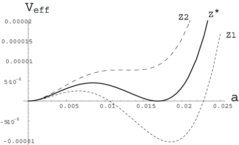
Figure 1: The behavior of the effective potential for the case (3) in the Table $4$. The critical temperature is given by $z^{*}=0.015345$ and $z1(z2)=0.01518(0.0155)$.

We list the numerical result in the Table 4. The critical temperature (measured in GeV) is obtained by

$$T_{c}\equiv{z^{*}\over R}=z^{*}\left({v\over a_{0}}\right)g_{4}\sim z^{*}\left({v\over a_{0}}\right)~{}~{}\mbox{for}~{}~{}g_{4}\sim O(1),$$ (3.21)

where $v\simeq 246$ GeV and $a_{0}$ is determined as the minimum of the zero temperature effective potential. The critical values of $a_{T_{c}}$ is obtained numerically and it yields

$${v(T_{c})\over T_{c}}={1\over T_{c}}{a_{T_{c}}\over{g_{4}R}}={1\over g_{4}}{{a_{T_{c}}}\over z^{*}}\sim{{a_{T_{c}}}\over z^{*}}~{}~{}\mbox{for}~{}~{}g_{4}\sim O(1).$$ (3.22)

We observe that the bulk mass actually weakens the first order phase transition. If we compare the cases $(2)$-$(6)$ with the case $(1)$, we see that the quantity $v(T_{c})/T_{c}$ for $(2)$-$(6)$ is smaller than that of the case $(1)$. This shows that massive fields tend to weaken the first order phase transition, which is consistent with the common belief.

The result of the case $(7)$ is somewhat exceptional case. All the field but the gauge field is essentially massive in this case, so that we do not expect the strong first order phase transition. Due to the slightly large bulk mass, however, the fields with such large bulk mass do not contribute to the effective potential because of the Boltzmann like suppression factor in the modified Bessel function, $K_{5/2}({M\over{T}}\sqrt{(nLT)^{2}+l^{2}})$. The five dimensional gauge fields dominates in the effective potential and gives the main contribution to the cubic term. That’s why we have the strong first order phase transition. As we have explained in the previous paper [13], the Higgs mass in this case is lighter because of the $z^{2}$-suppression in the logarithmic factor.

As for the results in Table 4, we can also see that the bulk mass weaken the first order phase transition by comparing the results (2)-(5) with that of (1). However, thanks to the scalar fields with periodic boundary conditions (specified by the flavor number $N_{fd}^{(+)s}$), the coefficients of the cubic term of the Higgs potential is enhanced. Thus, we can still obtain the strong first order phase transition although the bulk mass weakens the strength of the first order phase transition. This is the crucial difference between the case (A) and the case (B). In Figure 1, we depict the behavior of the effective potential at finite temperature for the case (3) in the Table 4. And this is a typical behavior for the first order phase transition obtained in the analyses.

We also find that there is an interesting behavior in this case. For the case (2), we have $m_{H}\simeq 118.58(\sim 118.6)$ GeV with $v(T_{c})/T_{c}\simeq 1.0949(\sim 1.10)$. On the other hand, for the case (3), we have $m_{H}\simeq 119.63(\sim 120)$ GeV with $v(T_{c})/T_{c}\simeq 1.0985(\sim 1.10)$. Even though it is a tiny difference, contrary to the common sense, the heavier Higgs really induces the stronger first order phase transition. This is also considered to be the effect of the bulk mass on the phase transition.

4 Conclusion

In this paper, we have investigated the bulk mass effects on the electroweak phase transition at finite temperature in the five dimensional SU(3) gauge-Higgs unification theory, in particular the compatibility of the Higgs mass satisfying the experimental lower bound and the strong first order phase transition necessary for a successful electroweak baryogenesis.

It is known that in general the massive matter and fermion tend to weaken the first order phase transition, so that we expect the bulk mass does not enhance the first order phase transition. This is actually the case in our numerical studies. If the model contains the zero mode for scalar field like in the case (B), we can still have the strong first order phase transition.

Our numerical results in this paper show that the matter content of the case (B) is favorable, where the Higgs mass is above the lower bound and the electroweak baryogenesis works well. This is the reason why the scalar fields with periodic boundary condition included only in the case (B) give the contributions for the cubic term in the effective potential and enhance the strength of the first order phase transition. From the experimental point of view, the case (B) is also interesting in that the Higgs mass is predicted to be close to the lower bound.

In the standard argument of the Higgs mass and the order of the phase transition, it is known that the lighter Higgs tends to give the stronger first order phase transition. This is also understood from Eqs. (3.18) and (3.19). In our examples studied in this paper, namely, the cases (2) and (3) in (B), we found an interesting behavior that the heavier Higgs gives the stronger first order phase transition. This behavior helps us to construct realistic models.

In this paper, we have not addressed another important issue in gauge-Higgs unification, namely the problem of too small top mass. In gauge-Higgs unification, Yukawa coupling is dictated by the gauge coupling. Therefore, it is nontrivial to generate the order one coupling, such as the top Yukawa coupling. Recent proposal on this issue were made by [7] in terms of large representation fermions and [8] in terms of an explicit violation of 5D Lorenz invariance. It would be very interesting to examine whether the top mass can be obtained without spoiling the good points obtained in our analysis. This is left for a future work.

References

• [1] N. S. Manton, Nucl. Phys. B 158, 141 (1979); D. B. Fairlie, Phys. Lett. B 82, 97 (1979).
• [2] N. V. Krasnikov, Phys. Lett. B 273 (1991) 246; N. Arkani-Hamed, A. G. Cohen and H. Georgi, Phys. Lett. B 513, 232 (2001); G. R. Dvali, S. Randjbar-Daemi and R. Tabbash, Phys. Rev. D 65, 064021 (2002);
• [3] H. Hatanaka, T. Inami and C. S. Lim, Mod. Phys. Lett. A 13, 2601 (1998);
• [4] I. Antoniadis, K. Benakli and M. Quiros, New J. Phys.  3, 20 (2001).
• [5] Y. Hosotani, Phys. Lett. B 126, 309 (1983), Annals Phys.  190, 233 (1989).
• [6] K. Takenaga, Phys. Rev. D 64, 066001 (2001); Phys. Rev. D 66, 085009 (2002); L. J. Hall, Y. Nomura and D. R. Smith, Nucl. Phys. B 639, 307 (2002); M. Kubo, C. S. Lim and H. Yamashita, Mod. Phys. Lett. A 17, 2249 (2002); C. Csaki, C. Grojean and H. Murayama, Phys. Rev. D 67, 085012 (2003); G. Burdman and Y. Nomura, Nucl. Phys. B 656, 3 (2003); N. Haba and Y. Shimizu, Phys. Rev. D 67, 095001 (2003) [Erratum-ibid. D 69, 059902 (2004)]; C. A. Scrucca, M. Serone and L. Silvestrini, Nucl. Phys. B 669, 128 (2003); K. W. Choi, N. Haba, K. S. Jeong, K. i. Okumura, Y. Shimizu and M. Yamaguchi, JHEP 0402, 037 (2004); N. Haba, Y. Hosotani, Y. Kawamura and T. Yamashita, Phys. Rev. D 70, 015010 (2004); N. Haba, K. Takenaga and T. Yamashita, Phys. Rev. D 71, 025006 (2005); G. Martinelli, M. Salvatori, C. A. Scrucca and L. Silvestrini, JHEP 0510, 037 (2005); I. Gogoladze, T. Li, Y. Mimura and S. Nandi, Phys. Rev. D 72, 055006 (2005); N. Haba, S. Matsumoto, N. Okada and T. Yamashita, JHEP 0602, 073 (2006).
• [7] G. Cacciapaglia, C. Csaki and S. C. Park, JHEP 0603, 099 (2006);
• [8] G. Panico, M. Serone and A. Wulzer, Nucl. Phys. B 739, 186 (2006);
• [9] R. Contino, Y. Nomura and A. Pomarol, Nucl. Phys. B 671, 148 (2003); K. Agashe, R. Contino and A. Pomarol, Nucl. Phys. B 719, 165 (2005); K. y. Oda and A. Weiler, Phys. Lett. B 606, 408 (2005); Y. Hosotani and M. Mabe, Phys. Lett. B 615, 257 (2005); Y. Hosotani, S. Noda, Y. Sakamura and S. Shimasaki, Phys. Rev. D 73, 096006 (2006).
• [10] K. Takenaga, Phys. Lett. B 570, 244 (2003); N. Haba, K. Takenaga and T. Yamashita, Phys. Lett. B 605, 355 (2005).
• [11] G. Panico and M. Serone, JHEP 0505, 024 (2005).
• [12] N. Maru and K. Takenaga, Phys. Rev. D 72, 046003 (2005).
• [13] N. Maru and K. Takenaga, Phys. Lett. B 637, 287 (2006).
• [14] N. Maru and T. Yamashita, arXiv:hep-ph/0603237.
• [15] C. S. Lim, N. Maru and K. Hasegawa, arXiv:hep-th/0605180.
• [16] G. von Gersdorff, N. Irges and M. Quiros, Nucl. Phys. B 635, 127 (2002).
• [17] Y. Hosotani, S. Noda and K. Takenaga, Phys. Lett. B 607, 276 (2005);
• [18] K. Hasegawa, C. S. Lim and N. Maru, Phys. Lett. B 604, 133 (2004).
• [19] C. Csaki, C. Grojean and H. Murayama; G. Burdman and Y. Nomura; C. A. Scrucca, M. Serone and L. Silvestrini in [6].
• [20] S. R. Coleman and E. Weinberg, Phys. Rev. D 7, 1888 (1973).
• [21] K. Funakubo, A. Kakuto and K. Takenaga, Prog. Theor. Phys.  91, 341 (1994).
• [22] L. Dolan and R. Jackiw, Phys. Rev. D 9, 2904 (1974).
• [23] A. G. Cohen, D. B. Kaplan and A. E. Nelson, Ann. Rev. Nucl. Part. Sci.  43, 27 (1993); K. Funakubo, Prog. Theor. Phys.  96, 475 (1996); V. A. Rubakov and M. E. Shaposhnikov, Usp. Fiz. Nauk 166, 493 (1996) [Phys. Usp.  39, 461 (1996)].