Abstract

Among the firm predictions of softly broken supersymmetry is the identity of gauge couplings and the corresponding Yukawa couplings between gauginos, sfermions and fermions. In the event that a SUSY-like spectrum of new particles is discovered at future colliders, a key follow-up will be to test these relations experimentally. In detailed studies it has been found that the SUSY-Yukawa couplings of the electroweak sector can be studied with great precision at the ILC, but a similar analysis for the Yukawa coupling of the SUSY-QCD sector is far more challenging. Here a first phenomenological study for determining this coupling is presented, using a method which combines information from LHC and ILC.

1 Introduction

With more than 1 fb^-1 of luminosity on tape at the Tevatron experiments, and with the LHC and ILC on the horizon, TeV scale physics is fast entering the realm of experimental study. Among the most interesting and comprehensively studied possibilities for observable new physics is supersymmetry (SUSY). Interesting in its own right by virtue of being the largest possible space-time symmetry [1], it was chiefly with a number of additional theoretical successes in the early eighties that supersymmetry gained widespread acceptance, among these successful gauge coupling unification, radiative breaking of electroweak symmetry, and a natural candidate for Dark Matter.

Stated briefly, supersymmetry promotes all the fields of the Standard Model (SM) to superfields, all its multiplets to supermultiplets. Each such multiplet contains one boson and one fermion, which are related to each other by supersymmetry. Hence not only should all the SM particles (including at least one more Higgs doublet) have ‘sparticle’ superpartners, with spins differing by 1/2, but also the interactions of these superpartners should be fixed by supersymmetry. Even when considering broken supersymmetry (the only phenomenologically viable option), many of these relations persist, or are only modified to a tractable degree. Hence, part of the effort of testing the hypothesis, should suitable particles be discovered, will be to check whether their interactions do obey the supersymmetric relations or not. It is the feasibility of a particular such study we shall address here.

Among the most intuitively clear relations is that the supersymmetric partner of a gauge boson, a gaugino, must couple with the same strength to gauge charge as its partner does. That is, the Yukawa coupling $\hat{g}$ between a gaugino interacting with a fermion and a sfermion must be identical to the corresponding SM gauge coupling $g$ between a gauge boson and two (s)fermions. More specifically, denoting an SM fermion (gauge boson) by $f$ ($V$), and its sfermion (gaugino) superpartner by $\tilde{f}$ ($\tilde{V}$),

$$g \equiv g(Vff)=g(V{\tilde{f}}{\tilde{f}}), \hat{g} \equiv g(\tilde{V}f{\tilde{f}})~{},$$ (1)

with

$$g=\hat{g}$$ (2)

required by supersymmetry. Indeed this relation is vital for the cancellation of quadratic divergencies in the radiative corrections to the Higgs mass.

In what follows, we now constrain our attention to the Minimal Supersymmetric Extension of the Standard Model (MSSM), with $CP$ and $R$-parity conserved. Hence the Lightest Supersymmetric Particle (LSP), usually the lightest neutralino, is stable, and supersymmetric particles can only be produced in pairs.

If the supersymmetric particles are light enough to be produced at the next generation of colliders, it has been shown [2] that the supersymmetric Yukawa couplings in the electroweak sector can be precisely tested at a high-energy $e^{+}e^{-}$ collider. The $t$-channel contributions to neutralino/chargino [3] and slepton production [2, 4, 5] in $e^{+}e^{-}$ and $e^{-}e^{-}$ collisions are directly dependent on the U(1) and SU(2) Yukawa couplings. From measurements of total and differential cross sections, these couplings can thus be extracted with a precision at the per-cent level [2, 4, 5].

However, the analysis of the supersymmetric Yukawa coupling $\hat{g}_{\rm s}$ in the SU(3) QCD sector is much more difficult. At the ILC this interaction can be studied in the process $e^{+}e^{-}\to q{\tilde{q}}^{*}\tilde{g}$, $\bar{q}{\tilde{q}}\tilde{g}$ [6]. While this approach is in principle straightforward, it suffers both from a very small cross section, at most about 1 fb for squark and gluino masses of a few hundred GeV [6], and also from the daunting challenge of selecting the signal from much larger $t\bar{t}$ and squark backgrounds. At the LHC on the other hand, squarks and gluinos with masses below 2–3 TeV are copiously produced, and their pair production cross sections depend directly on the supersymmetric Yukawa coupling $\hat{g}_{\rm s}$. However, measurements of total cross sections are exceedingly difficult in this environment, with typically only one or two specific decay channels of the squarks and gluinos experimentally accessible [7].

Here we consider a combination — the relevant branching ratios are to be determined at an $e^{+}e^{-}$ collider and combined with exclusive cross section measurements in selected channels at the LHC. Together, this information determines the total squark or gluino production cross section, from which a value for the SUSY-QCD Yukawa coupling $\hat{g}_{\rm s}$ can be extracted.

In this publication, a first analysis is presented to explore whether such a coherent LHC/ILC analysis can provide a useful determination of the SU(3) Yukawa coupling. Since it is not clear a priori that the goal is achievable at all, we constrain our attention to a rather optimistic scenario in this study, with reasonably low masses, large cross sections, and a fairly large squark-gluino mass splitting.

In the next section, the production of squarks at the LHC is studied and the basic phenomenology laid out. The relevant branching ratios of the squarks and how they could be determined from squark pair production at $e^{+}e^{-}$ colliders is the topic of section 3. We round off by presenting the combined result (in the particular scenario studied here) and give a few concluding remarks.

2 Squark production at the LHC

2.1 Phenomenology and Strategy – LHC

In $pp$ collisions, squark and gluino production occurs in a variety of combinations, often with both $s$- and $t$-channel diagrams as well as several different partonic initial states contributing to the same final state. Fig. 1 contains a condensed summary of these, with explicit illustration of which vertices go with the QCD gauge (dots) and Yukawa (squares) couplings, respectively.

  

           

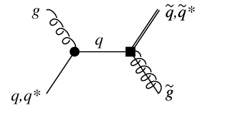
Figure 1: Some examples for Feynman diagrams for partonic squark and gluino production in hadron collisions. Dots indicate the gauge coupling $g_{\rm s}$, while squares stand for the Yukawa coupling $\hat{g}_{\rm s}$.

Naively, there are several processes from which one might attempt to extract the Yukawa coupling. However, final states which receive contributions from both gauge and Yukawa couplings make the analysis more complicated and model-dependent. To isolate the Yukawa coupling, we note that the production of same-sign squarks (e.g. ${\tilde{u}_{\rm L}}{\tilde{u}_{\rm L}}$, ${\tilde{u}_{\rm R}}{\tilde{u}_{\rm R}}$, …) proceeds only through the diagram shown in the lower left corner of Fig. 1, if one neglects the much smaller electroweak contributions. Hence, to excellent approximation, this process depends solely on the supersymmetric Yukawa coupling $\hat{g}_{\rm s}$, and to the extent it can be isolated from the background, a clean determination of $\hat{g}_{\rm s}$ should be possible. Note that, since the final state flavours are locked to the initial state ones, in $pp$ collisions this process dominantly produces ${\tilde{u}}$ and ${\tilde{d}}$ squarks, with smaller admixtures of sea-flavoured squarks, in direct proportion to the quark content of the proton at the relevant $x$ and $Q^{2}$ values.

Due to the flavour locking, only the first two generations of squarks are thus relevant, for which mixing effects are small and we can take mass and current eigenstates to be identical to good approximation. That is, the heavier ${\tilde{q}}$ mass eigenstate is pure ${\tilde{q}_{\rm L}}$ (weak isospin doublet), and the lighter one pure ${\tilde{q}_{\rm R}}$ (weak isospin singlet). Nominally, the lighter one would be the better target for a high-statistics study, simply due to phase space, but since it doesn’t couple to weak interactions, it decays almost exclusively via the hypercharge coupling to a same-flavour quark and the LSP. Since charge tagging for light-flavour jets is exceedingly difficult, this decay mode effectively obscures the fact that we had same-flavour squarks to begin with. Moreover, since it only contains a jet and missing energy, the mode would be extremely challenging to separate from the background. The only feasible avenue thus appears to be to use flavour/charge tagging modes of the heavier mass eigenstates, the ${\tilde{q}_{\rm L}}$.

For ${\tilde{q}_{\rm L}}$, the charge of the squark can be tagged through a chargino decay chain,

$${\tilde{u}_{\rm L}} \to d\,\tilde{\chi}^{+}_{1}\to d\,l^{+}\,\nu_{l}\,\tilde{\chi}^{0}_{1}, {\tilde{d}_{\rm L}} \to u\,\tilde{\chi}^{-}_{1}\to u\,l^{-}\,\bar{\nu}_{l}\,\tilde{\chi}^{0}_{1},$$ (3)

$${\tilde{u}_{\rm L}}^{*} \to\bar{d}\,\tilde{\chi}^{-}_{1}\to\bar{d}\,l^{-}\,\bar{\nu}_{l}\,\tilde{\chi}^{0}_{1}, {\tilde{d}_{\rm L}}^{*} \to\bar{u}\,\tilde{\chi}^{+}_{1}\to\bar{u}\,l^{+}\,\nu_{l}\,\tilde{\chi}^{0}_{1},$$ (4)

and similarly for ${\tilde{s}_{\rm L}}$ and ${\tilde{c}_{\rm L}}$. For a given squark flavor, the sign of the final-state lepton is related to the charge of the (anti-)squark. The production of same-sign squarks through the diagram in the lower left corner of Fig. 1 with this decay channel will therefore lead to same-sign leptons in the final state, while other direct squark production processes will tend to produce opposite-sign leptons in the final state. At this level, the signal is thus characterized by two same-sign leptons, two hard jets and missing transverse energy in the final state.

A very problematic background can come from gluino pair and mixed gluino-squark production if $m_{\tilde{g}}>m_{{\tilde{q}_{\rm L}}}$. In this case, gluinos can decay into quarks and squarks, $\tilde{g}\to q\,{\tilde{q}_{\rm L}}$, generating a component of two same-sign squarks plus additional jets which has a much more complicated (see Fig. 1) dependence on both the QCD gauge coupling and the Yukawa coupling we are interested in. This background becomes particularly challenging if the mass difference $m_{\tilde{g}}-m_{{\tilde{q}_{\rm L}}}$ is small, since then the additional jets from the gluino decay will be soft. Due to the large overall mass scale in the process, the bulk of the cross section will contain several extraneous QCD jets, e.g. from initial state radiation, which can be significantly harder than this [8], and hence the separation of squark production into direct and gluino-induced samples will be extremely non-trivial.

In the following we will only consider a scenario where the $m_{\tilde{g}}-m_{{\tilde{q}_{\rm L}}}$ mass difference is sufficiently large to allow a veto on additional jets for gluino background reduction. Although this will also reduce the signal somewhat, there are indications [8] that the particular signal process considered here, being dominated by valence quarks in the initial state, is associated with less extra radiation than other SUSY processes, which generally (in $pp$) have one or more gluons and/or sea quarks as initiators.

The most important backgrounds from Standard Model sources are $W^{\pm}W^{\pm}jj$ (same-sign $W$’s), where $j$ is a light-flavour jet, and semi-leptonic $t\bar{t}$, with the second lepton coming from the decay of a bottom quark. Due to the large total $t\bar{t}$ cross section, this can result in a sizable background. Below we include both these sources in our estimates, though the level of sophistication is obviously not anywhere near what would be required for a real experimental analysis.

2.2 Numerical Results – LHC

For the numerical analysis we use the scenario given in the appendix. This scenario is similar to the Snowmass point SPS1a [9], with the exception that the gluino mass is raised to 700 GeV. Since $\tan\beta=10$, the lightest scalar tau eigenstate has a sizeable left-handed component, and since the other left-handed sleptons are too heavy, the chargino mainly decays into scalar taus, which subsequently decay into taus. To trace the charge explicitly, we here restrict our attention only to the leptonic tau branching fraction. The decay chain for the signal process is then

$${\tilde{u}_{\rm L}} \stackrel{{\scriptstyle 65\%}}{{-\!\!\!-\!\!\!\longrightarrow}} d\,\tilde{\chi}^{+}_{1}\stackrel{{\scriptstyle 100\%}}{{-\!\!\!-\!\!\!\longrightarrow}}d\,\tau^{+}\,\nu_{\tau}\,\tilde{\chi}^{0}_{1}\stackrel{{\scriptstyle 35\%}}{{-\!\!\!-\!\!\!\longrightarrow}}d\,\ell^{+}+{\not{\!\!E}},$$

$${\tilde{d}_{\rm L}} \stackrel{{\scriptstyle 61\%}}{{-\!\!\!-\!\!\!\longrightarrow}} u\,\tilde{\chi}^{-}_{1}\stackrel{{\scriptstyle 100\%}}{{-\!\!\!-\!\!\!\longrightarrow}}u\,\tau^{-}\,\bar{\nu}_{\tau}\,\tilde{\chi}^{0}_{1}\stackrel{{\scriptstyle 35\%}}{{-\!\!\!-\!\!\!\longrightarrow}}u\,\ell^{-}+{\not{\!\!E}},\qquad\ell=e,\,\mu.$$ (5)

The numbers above the arrows indicate branching fractions and ${\not{\!\!E}}$ stands for missing energy.

Both signal and top and gluino backgrounds were simulated with Pythia 6.326 [10], i.e. with the hard $2\to 2$ scattering process calculated at leading order, dressed up with sequential resonance decays, parton showers (virtuality-ordered ‘power’ showers), underlying event (‘Tune A’ [11]), string hadronisation, and hadron decays (the $\pi^{0}$ was set stable to optimize efficiency). The $WWjj$ background was generated with MadEvent [12], i.e. at leading order with stable outgoing $W$ bosons and no fragmentation.

The cross sections for squark and gluino production were normalized by the $K$-factors obtained with Prospino 2.0 [13], which includes next-to-leading order QCD corrections. Top production was likewise normalized to a total inclusive LHC cross section of 800 pb, while for the $W^{\pm}W^{\pm}jj$ background only leading order results are available, translating to a comparatively larger theoretical uncertainty on this contribution. We further used Pythia to estimate the possible contamination from $VV$ ($ZZ$, $W^{\pm}Z$, and $W^{+}W^{-}$) production, and found it to be small.

Finally, a mock detector was set up, based on a toy calorimeter spanning the pseudorapidity range $|\eta|<5$ with a resolution of $0.1\times 0.1$ in $\eta\times\phi$ space and a primitive UA1-like cone jet algorithm, with a cone size of $\Delta R=0.4$. Muons and electrons were reconstructed inside $|\eta|<2.5$ and an isolation criterion was further imposed, requiring both less than 10 GeV of additional energy deposited in a cone of size $\Delta R=0.2$ around the lepton and also no reconstructed jets with $p_{\rm T,j}>25$ GeV closer than $\Delta R=0.4$ around the lepton. These criteria duplicate the default settings of the ATLFAST simulation package [14].

Based on the general characteristics of the squark signal, we chose a set of preselection cuts, to broadly define the signal region:

• at least 100 GeV of missing energy.

• at least 2 jets with $p_{\rm T,j}>100$ GeV.

• Exactly two isolated leptons $\ell=e,\mu$ with $p_{\rm T,\ell}>7$ GeV.

As evident from Tab 1, after preselection most backgrounds are still much larger than the same-sign squark signal. The backgrounds can be further reduced by making use of the following characteristics.

Cross Sections		Signal	Backgrounds
$\sum_{q=u,d,s,c}\sigma$ (fb)		${\tilde{q}_{\rm L}}{\tilde{q}_{\rm L}}$	Sum	$t\bar{t}$	$W^{\pm}W^{\pm}jj$	${\tilde{q}_{\rm L}}\tilde{g}$	${\tilde{q}_{\rm L}}{\tilde{q}_{\rm L}}^{*}$	$\tilde{g}\tilde{g}$
Total		2100	-	8$\times 10^{5}$	-	7000	1350	3200
Preselection		49.2	384.6	177.7	-	136.4	23.2	47.3
b-veto		17.1	31.4	13.0	-	10.3	7.1	1.0
${\not{\!\!E}}>150$ GeV		15.1	22.2	6.1	-	9.0	6.2	0.9
A)	$p_{T,j_{3}}<75$ GeV	10.1	9.5	3.6	N/A	2.3	3.5	0.1
	$p_{T,j_{1}}>200$ GeV	8.9	$<$7.6	1.7	$<$0.7	2.0	3.2	0.1
B)	$p_{T,j_{3}}<50$ GeV	7.8	5.9	2.4	N/A	1.0	2.5	0.03
	$p_{T,j_{1}}>200$ GeV	7.0	$<$4.9	1.0	$<$0.7	0.8	2.3	0.03
	($Q_{\ell}=+1$)	4.8	$<$3.0	0.6	$<$0.5	0.5	1.4	0.01

Table 1: Total and progressively reduced cross sections estimated from the cuts defined in the text, for the signal, summed background, and individual backgrounds, respectively. Two different sets of cuts have been considered, A and B, the latter incorporating a more severe 3rd jet veto. For illustration, the effect of including a further cut on the lepton sign is included for set B, though note that this last cut is not actually made in the analysis.

2.2.1 Cuts — Set A

The signal is flavour-locked to the initial state and hence contains almost no heavy-flavour squarks. On the other hand, both $t\bar{t}$ and $\tilde{g}\tilde{g}$ backgrounds contain large $b$ fractions (it is a general feature of models with universal high-scale squark masses that gluinos decay dominantly into third-generation squarks).

The number of $b$ jets (inside $|\eta|<5$ and with $p_{T}>25$ GeV) which would be identified with a perfect $b$ tagger is plotted in Fig. 2a. In reality, $b$ tagging is a trade-off between efficiency $\epsilon$ and mistagging rate $D$. Following the ATLAS Physics TDR [14] we investigated the performance of three different b taggers; one, Fig. 2b, with a large efficiency $\epsilon=90$% making it efficient against the background, but also high mistagging $D=25$% rate, making it expensive on the signal, a second, Fig. 2c, with $\epsilon=80$% and $D=10$%, and finally a third with $\epsilon=60$% and $D=2$%.

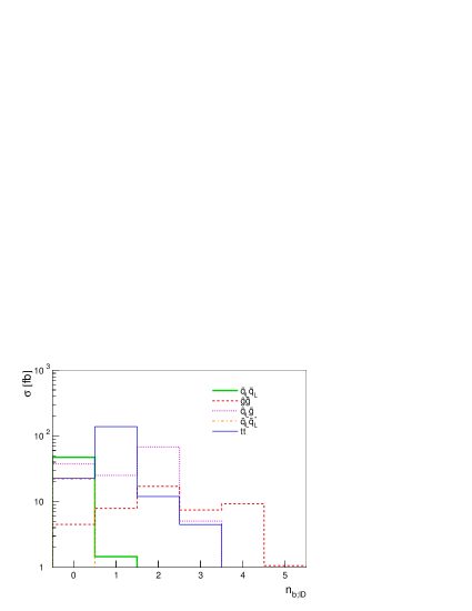
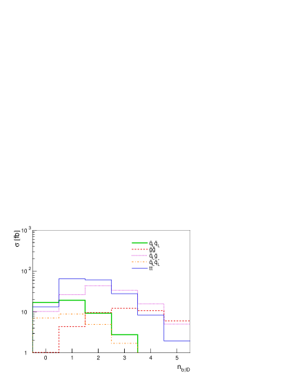
(a) $\epsilon=100$% ; $D=0$%	(b) $\epsilon=90$% ; $D=25$%
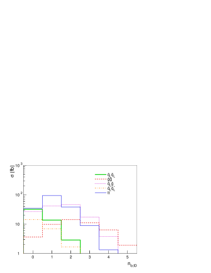
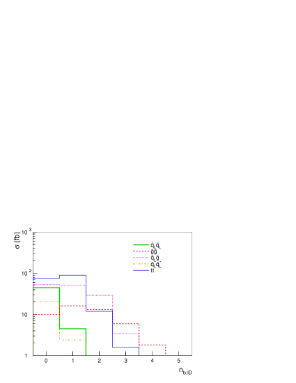
(c) $\epsilon=80$% ; $D=10$%	(d) $\epsilon=60$% ; $D=2$%

Figure 2: Distribution of number of $b$ tags for the 4 different taggers discussed in the text, (a) being an idealized tagger and (b)-(d) ATLAS-inspired ones.

For our purposes, the most important goal is to obtain as pure a signal as possible, and hence we choose the 0b bin of the highest efficiency tagger, Fig. 2b, for this analysis. For completeness, note that restricting the $b$ jet algorithm to the central detector region $|\eta|<2.5$ would not greatly affect our results; only a very small fraction of the true $b$ jets lie outside this region.

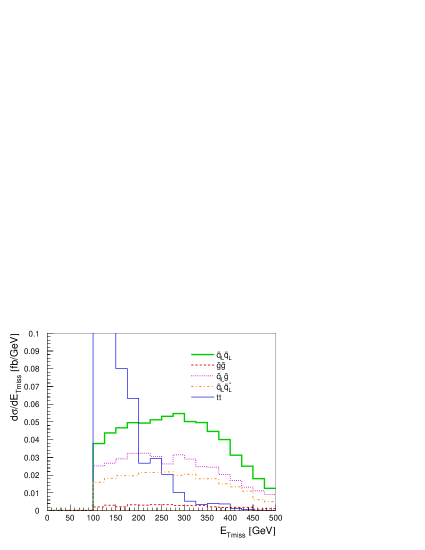
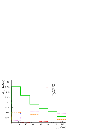
(a)	(b)

Figure 3: (a) Distribution of the missing transverse energy after cuts on b-tagging. The bins below 100 GeV are cut out by the preselection. (b) Distribution of the transverse momentum of the third jet after the cut on ${\not{\!\!E}}$.

Including now the $b$ jet veto, Fig. 3 shows the distribution of missing energy for the remaining events. While the contribution from top still dominates the background it can be effectively suppressed by increasing the ${\not{\!\!E}}$ cut. Here, we choose ${\not{\!\!E}}>150$ GeV.

At this point, the gluino-related backgrounds dominate. A veto on hard additional jets is essentially the only way of obtaining significant further rejection power against these. Fig. 3 (b) shows the distribution of the transverse momentum of the third-hardest jet for the events remaining in the analysis. By rejecting all events with $p_{\rm T,j3}>75$ GeV, the ratio of the signal to gluino background is markedly improved.

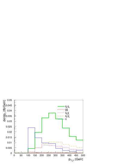
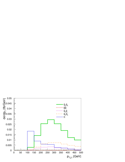
(a)	(b)

Figure 4: Distribution of the transverse momentum of the hardest jet after the third jet veto for (a) set A, and (b) set B. The bins below 100 GeV are cut out by the preselection.

The largest remaining background is now top production again (closely followed by ${\tilde{q}_{\rm L}}{\tilde{q}_{\rm L}}^{*}$), whose two hard jets tend to be softer than those of the signal, due to the large squark-chargino mass difference. This is illustrated in Fig. 4 (a), where the transverse momentum of the hardest jet in the remaining events is plotted.

Increasing the transverse momentum cut on the first jet to $p_{\rm T,j1}>200$ GeV we obtain a final signal cross section of 8.9 fb, over a background of less than 7.6 fb, with the effect of progressive cuts on signal and background normalisation and composition given in Tab. 1. The signal-to-background ratio is 1.2, sufficient to allow a meaningful measurement. With an integrated luminosity of 100 fb^-1, the statistical error on the same-sign squark cross section is 4.5%.

The reason we only quote an upper estimate of the background in Tab. 1 is that the $WWjj$ sample was not improved by parton showering, hence we have no way of estimating the effects of the 3rd jet veto on this component.

2.2.2 Harder Cuts — Set B

It is interesting to check if the situation can be improved by choosing stricter selection cuts. The gluino background can be further reduced by tightening the cuts on the third jet to $p_{\rm T,j3}<50$ GeV. In addition, the signal is dominated by up-squarks, since two out of three valence quarks of the proton are up-quarks. The $\tilde{q}\tilde{q}*$ background on the other hand needs at least one sea-quark in the initial state and therefore results in up- and down-squarks in more equal proportion. Thus the requirement of positively charged leptons in the final state will increase the ratio of same-sign squarks over opposite-sign squarks. With these stronger cuts the cross section values on the last line of Tab. 1 are obtained. Indeed the signal-to-background ratio is improved to 1.6, but at the cost of reduced overall statistics. We choose a compromise; omitting the final cut on lepton sign results in $S/B=1.45$, with acceptable statistics, yielding a signal cross section of 7 fb, over a total background of less than 4.9 fb. With a 100 fb^-1, the statistical error on the signal is 4.9%. This error is slighty larger than the result of the cuts Set A, but this is offset by lower background systematics (see section 4).

Noting that the two analyses are thus identical apart from the 3rd jet veto, one might ask why it is important to show the results of both. The reason, slightly touched on above and discussed in more detail in [8], is that 50 GeV jets are quite soft objects at the LHC, especially as compared to the signal scales we consider here, of order 600-700 GeV. Since we cannot be entirely sure that the parton shower resummation employed here is sufficiently accurate in this region, an explicit variation by a 25 GeV shift in the 3rd jet veto represents one way of verifying whether the analysis and thereby our conclusions are stable against variations of this cut.

3 Squark decays at an $e^{+}e^{-}$ collider

3.1 Phenomenology and Strategy – ILC

In order to interpret the measured rates at the LHC in terms of the total squark production cross section, the individual branching ratios in the decay chain eq. (5) need to be established. We now turn to a discussion of how each of these could be extracted from measurements at a high-energy $e^{+}e^{-}$ linear collider.

The chargino properties are the most straightforward to determine, being easily accessible via the chargino pair production process, $e^{+}e^{-}\to\tilde{\chi}_{1}^{+}\tilde{\chi}^{-}_{1}$. Due to the large rate for that process, the expected error on cross section measurements is about 1% at a 500 GeV collider [7]. Since the charginos $\tilde{\chi}^{\pm}_{1}$ are among the lightest supersymmetric particles, the only open decay channels are $\tilde{\chi}^{+}_{1}\to l^{+}\nu_{l}\,\tilde{\chi}^{0}_{1}$, $l=e,\mu,\tau$, which can all be easily separated from the background [7]. We therefore assume that the chargino branching ratios are known with 1% error: BR($\tilde{\chi}^{+}_{1}\to\tau^{+}\nu_{\tau}\tilde{\chi}^{0}_{1})=(100\pm 1)$%.

The squarks offer substantially more resistance. In the given scenario the left-squarks are in fact slightly too heavy to be accesible at a linear collider with 1 TeV center-of-mass energy. Rather than attempting to find a more amenable parameter point, we here consider the hypothetical case of an $e^{+}e^{-}$ collider with a center-of-mass energy of about 1.5 TeV. Obviously, we do not propose to address the technical challenges of such a machine, but justify our choice simply by the proof-of-concept nature of our study. We also assume that both beams can be polarized, with polarization degrees of 80% for electrons, and 50% for positrons.

Having kept the squarks heavy, we must now deal with the fact that they can decay into the whole spectrum of charginos and neutralinos. The heavier charginos and neutralinos have large branching ratios into gauge bosons, which distinguishes them from the lighter states. The following characteristic decay modes are chosen to distinguish the various charginos and neutralinos:

$$\tilde{\chi}^{+}_{1} \to\tau^{+}\nu_{\tau}\tilde{\chi}^{0}_{1},$$ BR=100% (6)

$$\tilde{\chi}^{+}_{2} \to Z\tilde{\chi}^{+}_{1}\to Z\,\tau^{+}\nu_{\tau}\,\tilde{\chi}^{0}_{1},$$ BR=24% (7)

$$\tilde{\chi}^{0}_{2} \to\tau\tau\,\tilde{\chi}^{0}_{1},$$ BR=100% (8)

$$\tilde{\chi}^{0}_{3,4} \to W^{\pm}\tilde{\chi}^{\mp}_{1}\to W^{\pm}\,\tau^{\mp}\nu_{\tau}\tilde{\chi}^{0}_{1}.$$ BR=59%,52% (9)

A distinction of the $\tilde{\chi}^{0}_{3}$ and $\tilde{\chi}^{0}_{4}$ states is not necessary since for the purpose of this study only the branching fraction into the lightest chargino needs to be known as an absolute number. The tau leptons in the final state can be identified in their hadronic decay mode with roughly 80% tagging efficiency. Since about 65% of tau decays are hadronic, this amounts to a total tau tagging efficiency of about 50%, consistent with the findings e.g. of LEP2 studies (see for instance Ref. [15]).

3.2 Numerical Results – ILC

For this work, Monte-Carlo samples for squark pair production in the different squark decay channels have been generated at the parton level with the tools of Ref. [5, 16]. Also the most relevant backgrounds have been simulated, stemming from double and triple gauge boson production as well as $t\bar{t}$ production. It is assumed that an integrated luminosity of 500 fb^-1 is spent for a polarization combination $P(e^{+})$/$P(e^{-})$ = +50%/$-$80%, which enhances the production cross section both for ${\tilde{u}_{\rm L}}$ and ${\tilde{d}_{\rm L}}$ production. Here $\mp$ indicates left/right-handed polarization. The branching fractions are obtained from measuring the cross sections of all accessible decay modes of the squarks and identifying the fraction of decays into one specific decay mode out of these.

Since the squarks are produced in charge-conjugated pairs, it is a priori difficult to distinguish up- and down-squarks in the final state. However, assuming universality between the first two generations, a separation between up- and down-type squarks can be obtained through charm tagging. According to Ref. [17], a $c$-tagging efficiency of 40% is achievable for a purity of 90%. By combining the different decay channels in eqs. (6–9), the following final state signatures are identified as interesting: $jj(n\tau){\not{\!\!E}}$ with $n\in\{1,2,3,4\}$, $cc(n\tau){\not{\!\!E}}$ with $n\in\{2,4\}$, $jj\tau\tau(Z/W){\not{\!\!E}}$, $cc\tau\tau Z{\not{\!\!E}}$, where $j$ indicates an untagged jet, $c$ a tagged charm jet, and $Z/W$ a hadronically decaying gauge boson where the invariant mass of the two jets combines to the given gauge boson mass. For charged current squark decays, charm tagging does not provide any additional information, since a $cs$+leptons final state can arise both from up- and down-type squarks. Therefore, only signatures with two tagged charm jets are included in the list above. Finally, since several squark decay channels can contribute to most of the final states above, one has to solve a linear equation system in order to derive the individual contributions.

Before presenting results for this procedure, there is an additional complication due to the subsequent decays of the neutralinos and charginos after the squark decays. The branching fractions for the light chargino $\tilde{\chi}^{\pm}_{1}$ and neutralino $\tilde{\chi}^{0}_{2}$ can be deduced from cross section measurements at a low-energy run with $\sqrt{s}=500$ GeV, as mentioned above. Only a few decay channels are kinematically open, and the environment is sufficiently clean so that all decay channels are easily visible with a small error.

The situation is more tedious for the heavier charginos and neutralino, which have many different decay channels open. Rather than attempting to measure individual cross sections for all these decay modes, here instead a different method is pursued. Near production threshold of two supersymmetric particles $\tilde{X}\tilde{Y}$, the energy of a particle from a two-body decay mode of e.g. $\tilde{X}$ is sharply defined. The signal of such a monoenergetic particle would clearly stand out over the background, which is smooth in the particle energy, and can thus be used to identify a particular production cross section irrespective of the decay mode of the other sparticle $\tilde{Y}$.

The branching ratios of the heavy neutralinos $\tilde{\chi}^{0}_{3,4}$ can be studied in associated production with $\tilde{\chi}^{0}_{2}$, $e^{+}e^{-}\to\tilde{\chi}^{0}_{2}\tilde{\chi}^{0}_{3,4}$. When approaching the production threshold, the decay of the $\tilde{\chi}^{0}_{2}$ is characterized by a monoenergetic $\tau$ lepton over a smooth background. The production threshold for $\tilde{\chi}^{0}_{2}\tilde{\chi}^{0}_{3}$ lies at $\sqrt{s}=m_{\tilde{\chi}^{0}_{2}}+m_{\tilde{\chi}^{0}_{3}}$, 535 GeV in the present case. A few GeV above this threshold, at $\sqrt{s}=540$ GeV, the production cross section is already sizeable, $\sigma_{23}(\sqrt{s}=540{\rm\ GeV})=15.8$ fb with polarized beams $P(e^{+})$/$P(e^{-})$ = +50%/$-$80%. The cross section for $\tilde{\chi}^{0}_{2}\tilde{\chi}^{0}_{4}$ is unfortunately too small to allow a meaningful measurement. An alternative is to obtain the branching fractions of $\tilde{\chi}^{0}_{4}$ at the $\tilde{\chi}^{0}_{3}\tilde{\chi}^{0}_{4}$ threshold, by tagging the $\tilde{\chi}^{0}_{3}$ decays into a monoenergetic $W$-boson. Of course for this purpose only hadronic $W$ modes can be used. A few GeV above the kinematical threshold $m_{\tilde{\chi}^{0}_{3}}+m_{\tilde{\chi}^{0}_{4}}=737$ GeV, the production cross section is relatively large, $\sigma_{34}(\sqrt{s}=745{\rm\ GeV})=29.3$ fb, assuming polarized beams as above.

For a full feasibility demonstration of this technique, a realistic detector simulation would be necessary. Here the achievable precision for the neutralino and chargino branching ratios is estimated by simulating the parton-level production near threshold. Assuming 50 fb^-1 luminosity for each of the threshold measurements, the following statistical errors are found:

$$\begin{gathered}{\rm BR}(\tilde{\chi}^{0}_{3}\to W^{\pm}\chi^{\mp}_{1})=(59\pm 6.5)\%,\qquad{\rm BR}(\tilde{\chi}^{0}_{4}\to W^{\pm}\chi^{\mp}_{1})=(52\pm 2.5)\%,\\ {\rm BR}(\tilde{\chi}^{\pm}_{2}\to Z\chi^{\pm}_{1})=(24\pm 1.3)\%.\end{gathered}$$ (10)

Together with this information, the squark cross section measurements at $\sqrt{s}=1.5$ TeV can be interpreted in terms of squark branching ratios. Solving the linear equations system that connects final state signatures with production processes with a $\chi^{2}$ scan, the estimated errors for the squark branching ratios are listed in Tab. 2.

${\tilde{u}_{\rm L}}\to u\tilde{\chi}^{0}_{1}$	$0.9\pm 0.5$ %	${\tilde{d}_{\rm L}}\to d\tilde{\chi}^{0}_{1}$	$1.9\pm 0.8$ %
$u\tilde{\chi}^{0}_{2}$	$29.0\pm 3.0$ %	$d\tilde{\chi}^{0}_{2}$	$28.3\pm 4.8$ %
$u\tilde{\chi}^{0}_{3}$	$<1$ %	$d\tilde{\chi}^{0}_{3}$	$<0.2$ %
$u\tilde{\chi}^{0}_{4}$	$<1$ %	$d\tilde{\chi}^{0}_{4}$	$1.9\pm 0.8$ %
$d\>\!\tilde{\chi}^{\mbox{\tiny+}\!}_{1}$	$67.7\pm 3.2$ %	$u\tilde{\chi}^{\mbox{\tiny$-$}\!}_{1}$	$63.9\pm 5.2$ %
$d\>\!\tilde{\chi}^{\mbox{\tiny+}\!}_{2}$	$1.4\pm 0.7$ %	$u\tilde{\chi}^{\mbox{\tiny$-$}\!}_{2}$	$4.0\pm 1.4$ %

Table 2: Estimated error for squark branching determination from measurements at an $e^{+}e^{-}$ collider with $\sqrt{s}=1.5$ TeV.

For the purpose of this work, the interesting information are the branching ratios of ${\tilde{u}_{\rm L}}$ and ${\tilde{d}_{\rm L}}$ into the light chargino $\tilde{\chi}^{\pm}_{1}$.

4 Combination – LHC and ILC

Based on the results from the simulations for squark production at the LHC and the ILC presented in the previous sections, one can now derive an estimate for the precision for the determination of the supersymmetric strong Yukawa coupling $\hat{g}_{\rm s}$. Since the production of same-sign squarks at the LHC with gluino $t$-channel exchange is proportional to $\sigma[{\tilde{q}_{\rm L}}{\tilde{q}_{\rm L}}]\propto\hat{g}_{\rm s}^{4}$, the error for the coupling constant $\hat{g}_{\rm s}$ is roughly one quarter of the error of the total same-sign squark production cross section at the LHC. The statistical uncertainty is combined with the most important systematic error sources in Tab. 3.

	$\sigma[{\tilde{q}_{\rm L}}{\tilde{q}_{\rm L}}]$	$\hat{g}_{\rm s}/g_{\rm s}$
LHC signal statistics	4.9%	1.3%
SUSY-QCD Yukawa coupling
in ${\tilde{q}_{\rm L}}\tilde{g}$ background	2.4%	0.6%
PDF uncertainty	10%	2.4%
NNLO corrections	8%	2.0%
Squark mass $\Delta m_{{\tilde{q}_{\rm L}}}=9$ GeV	6%	1.5%
BR$[{\tilde{q}_{\rm L}}\to q^{\prime}\,\tilde{\chi}^{\pm}_{1}]$	8.2%	2.0%
	17.3%	4.1%

Table 3: Combination of statistical and systematic errors for the determination of the absolute same-sign squark production cross section at the LHC and the derivation of the strong SUSY-Yukawa coupling. The cuts set B were used for the LHC.

The numbers are based on the choice (B) for the LHC signal selection in Tab. 1. We now turn to a discussion of the various unvertainties and caveats associated with these numbers.

The remaining background after selection cuts at the LHC introduces a systematic uncertainty since the supersymmetric background from gluino production also depends on $\hat{g}_{\rm s}$. Including the variation of $\hat{g}_{\rm s}$ in the dominant squark-gluino background introduces an uncertainty of 5% on the signal. The background from opposite-sign squark production is also sizeable, but depends in the same way on $\hat{g}_{\rm s}$ as the signal, $\sigma\propto\hat{g}_{\rm s}^{4}$ and thus does not introduce an additional systematic effect.

In order to determine absolute cross sections, the proton parton distribution functions (PDFs) in the relevant $x$ and $Q^{2}$ ranges must be known accurately. The production of same-sign squarks proceeds from same-sign quarks in the initial state and is therefore dominated by the contributions from valence quarks. The value of valence quark PDFs at high scattering energies can be computed reliably from perturbative parton evolution and can be checked against measurements of vector boson production. We tested this assumption by comparing results for different CTEQ PDFs releases (CTEQ6M, CTEQ6D, CTEQ5M1, CTEQ5L and CTEQ6L1) [18] and find a maximal variation of 7% in the signal and 4% in the background. Thus we assign a total error of 10% for the parton distributions.

Squark production receives large higher order QCD corrections. The next-to-leading order corrections are known [13] and can be included in the analysis. The uncertainty of the missing ${\cal O}(\alpha^{2}_{\rm s})$ contributions are estimated by varying the renormalization scale of the ${\cal O}(\alpha_{\rm s})$ corrected cross section between $m_{{\tilde{q}_{\rm L}}}/2<Q<2m_{{\tilde{q}_{\rm L}}}$, leading to an error of 8%. Furthermore the cross section depends on the values of the squark masses. According to Ref. [7], the left-chiral first generation squark masses can be determined with an error better than $\Delta m_{{\tilde{q}_{\rm L}}}=9$ GeV, leading to an uncertainty of about 6% for the production cross section. Finally, the expected error for the determination of the squark branching ratios at the linear collider must be included.

Combining all error sources in quadrature, it is found that the same-sign squark production cross section can be determined with an error of 17.3%, translating to an error of 4.1% for the supersymmetric QCD Yukawa coupling $\hat{g}_{\rm s}$. That is, assuming the steps outlined here can be carried out in more or less the fashion described, it should be possible to test the supersymmetry identity between gauge and Yukawa couplings to the level of a few percent.

It should be noted though that this result is highly scenario dependent. For different supersymmetric scenarios, with larger squark masses, smaller gluino masses or different squark decay modes, the analysis could be much more difficult or even impossible. It is also interesting to study gluino production not only as a background, but as a signal process for studying the SUSY-QCD Yukawa coupling, although this introduces additional complications since gluino production always depends both the the gauge and Yukawa couplings. Nevertheless we hope this study shows that the determination of the supersymmetric QCD Yukawa coupling with competetive precision is not out of reach, and that it is a tantalizing target for a complex all-embracing combination of LHC and lepton collider data.

5 Conclusion

We have described a phenomenological method for testing the identity between the QCD gauge coupling and the corresponding squark-gluino-quark Yukawa coupling that arises in supersymmetric theories. Noting that same-sign squark production at a hadron collider is both a very clean signal and also directly proportional to the fourth power of the QCD Yukawa coupling, we propose to measure the exclusive cross section for same-sign squark production at the LHC in a particular decay channel. To convert this to a measurement of the Yukawa coupling, branching fraction determinations at a future lepton collider are (de-)convoluted with the LHC measurement to yield a combined determination of the total inclusive cross section for same-sign squark production. We find that this cross section can be determined to roughly 20% precision, in the scenario studied here, translating to roughly 5% precision on the Yukawa coupling. This is certainly encouraging and, we hope, sufficient in itself to spark off more in-depth studies. Obviously, due to the complexity and breadth of the proposed analysis, we were forced to employ some shortcuts here, as described in detail in the text above. It would be highly interesting to establish how these estimates would compare to both a more detailed (in the sense of detector capabilities and systematic uncertainties) and comprehensive (in the sense of exploring a wider range of parameter space) analysis.

Appendix

Here the reference scenario is listed that is used in this analysis. It is coincides with the Snowmass point SPS1a [9], but has a larger gluino mass of 700 GeV. The scenario is defined at the weak scale through the supersymmetry breaking parameters. The parameters relevant for this work are

$$M_{1} =99{\rm\ GeV} \qquad\qquad m_{\rm L3} =197{\rm\ GeV} \qquad\qquad m_{\rm Q1} =540{\rm\ GeV}$$ (11)

$$M_{2} =193{\rm\ GeV} m_{\rm R3} =136{\rm\ GeV} m_{\rm U1} =522{\rm\ GeV}$$

$$M_{3} =700{\rm\ GeV} A_{\tau} =-254{\rm\ GeV} m_{\rm D1} =520{\rm\ GeV}$$

$$\mu =352{\rm\ GeV} \tan\beta =10.$$

The tree-level masses are computed from this to

$$m_{{\tilde{u}_{\rm L}}} =537{\rm\ GeV} \qquad\qquad m_{\tilde{\chi}^{0}_{1}} =96{\rm\ GeV}$$ (12)

$$m_{{\tilde{d}_{\rm L}}} =543{\rm\ GeV} m_{\tilde{\chi}^{0}_{2}} =177{\rm\ GeV}$$

$$m_{{\tilde{\tau}}_{1}} =133{\rm\ GeV} m_{\tilde{\chi}^{\pm}_{1}} =176{\rm\ GeV}$$

$$m_{\tilde{g}} =700{\rm\ GeV} m_{\tilde{\chi}^{0}_{3,4}} \sim 360{\rm\ GeV}.$$

References

- [1] R. Haag, J. T. Lopuszanski and M. Sohnius, Nucl. Phys. B 88, 257 (1975).
- [2] J. L. Feng, M. E. Peskin, H. Murayama and X. Tata, Phys. Rev. D 52, 1418 (1995).
-
[3]
S. Y. Choi, A. Djouadi, M. Guchait, J. Kalinowski, H. S. Song and P. M. Zerwas,
Eur. Phys. J. C 14, 535 (2000);
S. Y. Choi, J. Kalinowski, G. Moortgat-Pick and P. M. Zerwas, Eur. Phys. J. C 22, 563 (2001). -
[4]
M. M. Nojiri, K. Fujii and T. Tsukamoto,
Phys. Rev. D 54, 6756 (1996);
H. C. Cheng, J. L. Feng and N. Polonsky, Phys. Rev. D 57, 152 (1998). -
[5]
A. Freitas, A. von Manteuffel and P. M. Zerwas,
Eur. Phys. J. C 34, 487 (2004);
A. Freitas, A. von Manteuffel and P. M. Zerwas, Eur. Phys. J. C 40, 435 (2005). - [6] A. Brandenburg, M. Maniatis and M. M. Weber, in Proc. of the 10th International Conference on Supersymmetry and Unification of Fundamental Interactions (SUSY02), Hamburg, Germany (2002), hep-ph/0207278.
- [7] G. Weiglein et al. [LHC/LC Study Group], hep-ph/0410364.
-
[8]
T. Plehn, D. Rainwater and P. Skands,
hep-ph/0510144;
P. Skands, T. Plehn and D. Rainwater, hep-ph/0511306. - [9] B. C. Allanach et al., Eur. Phys. J. C 25 (2002) 113.
-
[10]
T. Sjöstrand, L. Lönnblad, S. Mrenna and P. Skands,
hep-ph/0308153;
T. Sjöstrand et al., Comput. Phys. Commun. 135, 238 (2001);
S. Mrenna, Comput. Phys. Commun. 101, 232 (1997). -
[11]
T. Sjöstrand and M. van Zijl,
Phys. Rev. D 36, 2019 (1987);
R. D. Field, CDF Note 6403, hep-ph-0201192; further recent talks available from webpage http://www.phys.ufl.edu/rfield/cdf . - [12] F. Maltoni and T. Stelzer, JHEP 0302, 027 (2003).
-
[13]
W. Beenakker, R. Höpker, M. Spira and P. M. Zerwas,
Nucl. Phys. B 492, 51 (1997);
T. Plehn, Prospino 2.0 [pheno.physics.wisc.edu/~plehn/prospino/prospino.html]. -
[14]
ALTAS Technical Design Report, Vol 1, CERN/LHCC-99-15, Chapt. 10;
E. Richter-Was, D. Froidevaux and L. Poggioli, ATL-PHYS-98-131 (1998). - [15] G. Abbiendi et al. [OPAL Collaboration], Phys. Lett. B 493, 249 (2000).
- [16] A. Freitas, D. J. Miller and P. M. Zerwas, Eur. Phys. J. C 21, 361 (2001).
- [17] S. M. Xella Hansen, M. Wing, D. J. Jackson, N. De Groot and C. J. S. Damerell, LC-PHSM-2003-061 [www-flc.desy.de/lcnotes/].
- [18] J. Pumplin, D. R. Stump, J. Huston, H. L. Lai, P. Nadolsky and W. K. Tung, JHEP 0207, 012 (2002).