Operator Product Expansion in the
Production and Decay of the $X(3872)$

Abstract

The $X(3872)$ seems to be a weakly-bound hadronic molecule whose constituents are two charm mesons. Its binding energy is much smaller than all the other energy scales in QCD. This separation of scales can be exploited through factorization formulas for production and decay rates of the $X$. In a low-energy effective field theory for the constituents of the $X$, the factorization formulas can be derived using the operator product expansion. The derivations are carried out explicitly for the simplest effective theory in which the constituents interact through a contact interaction that produces a large scattering length. The long-distance factors in the operator product expansions for various observables are calculated nonperturbatively in the interaction strength of the contact interaction. After renormalization of the coupling constant, all remaining ultraviolet divergences can be absorbed into the short-distance factors in the operator product expansions.

I Introduction

The $X(3872)$ is a narrow resonance near $3872$ MeV discovered by the Belle collaboration in 2003 through its decay into $J/\psi\,\pi^{+}\pi^{-}$ Choi:2003ue . Its existence was subsequently confirmed by the CDF, Babar, and D0 collaborations Acosta:2003zx ; Abazov:2004kp ; Aubert:2004ns . Its mass $M_{X}$ is extremely close to the threshold for the charm mesons $D^{0}$ and $\bar{D}^{*0}$ Olsen:2004fp :

$$M_{X}-(M_{D^{0}}+M_{D^{*0}})=+0.7\pm 1.1\;{\rm MeV}.$$ (1)

The $X(3872)$ is narrower than most of the known charmonium states Choi:2003ue :

$$\Gamma_{X}<2.3\;{\rm MeV}\hskip 28.45274pt(90\%\ {\rm C.L.}).$$ (2)

The observation of the decay $X\to J/\psi\,\gamma$ implies that the $X$ has charge conjugation quantum number $C=+$ Abe:2005ix . Analyses of the discovery decay mode $X\to J/\psi\,\pi^{+}\pi^{-}$, including the angular correlations between the $J/\psi$ and the pions and the $\pi^{+}\pi^{-}$ invariant mass distribution, strongly favor the spin and parity quantum numbers $J^{P}=1^{+}$ Abe:2005iy . These properties are compatible with the identification of $X$ as a weakly-bound molecule whose constituents are a superposition of charm meson pairs Tornqvist:2003na ; Close:2003sg ; Pakvasa:2003ea ; Voloshin:2003nt ; Wong:2003xk ; Braaten:2003he ; Swanson:2003tb ; Braaten:2004rw ; Tornqvist:2004qy ; Braaten:2004fk ; Swanson:2004pp ; Voloshin:2004mh ; Braaten:2004ai ; Braaten:2005jj ; AlFiky:2005jd ; Braaten:2005ai ; Suzuki:2005ha :

$$X=\frac{1}{\sqrt{2}}\left(D^{*0}\bar{D}^{0}+D^{0}\bar{D}^{*0}\right).$$ (3)

If this identification is confirmed, the $X(3872)$ would be the first unambiguously identified member of a new class of hadrons: mesonic molecules Bander:1975fb ; Voloshin:ap ; DeRujula:1976qd ; Nussinov:1976fg ; Tornqvist:1993ng .

If the $X(3872)$ is a weakly-bound mesonic molecule, it shares an important feature with the simplest baryonic molecule, the deuteron. Their binding energies are both small compared to the natural energy scale associated with the exchange of the lightest meson, the pion. That natural energy scale is $m_{\pi}^{2}/(2M_{12})$, where $M_{12}$ is the reduced mass of the two constituents. The binding energy 2.2 MeV of the deuteron is small compared to the natural scale of about 20 MeV. The measurement of the mass of the $X$ in Eq. (1) implies that its binding energy $(M_{D^{0}}+M_{D^{*0}})-M_{X}$ is between $-2.4$ MeV and $1.2$ MeV at the 90% confidence level. The small width in Eq. (2) further suggests that the mass of the $X$ must be below the threshold for the charm mesons: $M_{X}<M_{D^{0}}+M_{D^{*0}}$. Thus the binding energy of the $X$ is small compared to the natural scale of about 10 MeV. The deuteron has an S-wave coupling to its constituents, the proton and the neutron. The quantum numbers $J^{PC}=1^{++}$ of the $X$ implies that it also has an S-wave coupling to its constituents. The combination of the small binding energy compared to the natural energy scale and the S-wave coupling to the constituents implies that the deuteron and the $X(3872)$ have universal properties that are determined by the large scattering length $a$ of their constituents Braaten:2003he . The simplest example of a universal result is a simple formula for the binding energy of the molecule: $E_{X}=1/(2M_{12}a^{2})$. The universality of few-body systems with a large scattering length has many applications in atomic, nuclear, and particle physics Braaten:2004rn . The universal features of the $X(3872)$ were first exploited by Voloshin to describe its decays into $D^{0}\bar{D}^{0}\pi^{0}$ and $D^{0}\bar{D}^{0}\gamma$, which can proceed through decay of the constituent $D^{*0}$ or $\bar{D}^{*0}$ Voloshin:2003nt . Universality has also been applied to the production process $\Upsilon(4S)\to\pi^{+}\pi^{-}+X$ Braaten:2004rw , to the production process $B\to K+X$ Braaten:2004fk ; Braaten:2004ai , to the line shape of the $X$ Braaten:2005jj , and to decays of $X$ into $J/\psi$ and pions Braaten:2005ai .

The tiny binding energy of the $X(3872)$ provides a new energy scale that is much smaller than the other scales in QCD, including the pion mass $m_{\pi}$ and the scale $\Lambda_{QCD}$ associated with nonperturbative effects. In Ref. Braaten:2005jj , this separation of scales was exploited by using factorization formulas to separate certain observables into long-distance factors that involve only energy scales comparable to the binding energy and short-distance factors that involve all the higher energy scales of QCD. The long-distance factors can be calculated using an effective field theory for the constituents of the $X$ that describes the lowest energy scale.

In this paper, we show how the factorization formulas can be derived using the operator product expansion for the effective field theory that describes the constituents of the $X$. The effective field theory that describes the $X(3872)$ is complicated by the spin 1 of the constituent $D^{*0}$ and by its charge conjugation quantum number $C=+$, which implies that it is the superposition of $D^{*0}\bar{D}^{0}$ and $D^{0}\bar{D}^{*0}$ given in Eq. (3). Another complication is that the $D^{0}\bar{D}^{0}\pi^{0}$ threshold is only about 8 MeV below the $D^{*0}\bar{D}^{0}$ threshold Suzuki:2005ha . We will therefore illustrate the operator product expansion formalism using a simpler model in which these complications are absent. The simplest such model is a scalar meson model in which the constituents are spin-0 mesons with a contact interaction that gives a large positive scattering length $a$. The generalization to a realistic model with charm mesons is then straightforward.

In Sec. II, we define the minimal charm meson model that can describe the $X(3872)$ and the simpler scalar meson model. In Sec. III, we explain how the operator product expansion can be used to separate scales in short-distance production and decay rates. In Sec. IV, we give exact nonperturbative results for long-distance observables in the scalar meson model. In Sec. V, we apply the operator product expansion to short-distance production and decay rates in the scalar meson model and we calculate the long-distance factors in the operator product expansion. We show that after renormalization of the coupling constant, all remaining dependence on the ultraviolet cutoff can be eliminated by renormalization of Wilson coefficients in the operator product expansion. In Sec. VI, we show how the factorization formulas can be simplified by expanding in inverse powers of the large scattering length. In Sec. VII, we extend the results of Secs. IV, V, and VI to the charm meson model. We summarize our results in Sect. VIII.

II Effective field theories

In this section, we define the scalar meson model and the minimal charm meson model. Both of these effective field theories have an S-wave bound state. We introduce interpolating fields for the S-wave bound states.

II.1 Scalar Meson Model

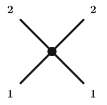
Figure 1: Vertex for the $D_{1}D_{2}$ contact interaction.

We will illustrate the derivation of factorization formulas using the operator product expansion in a simpler model that we call the scalar meson model. This model has an S-wave bound state which we will refer to as $X$. The constituents of the bound state are scalar mesons $D_{1}$ and $D_{2}$ with masses $M_{1}$ and $M_{2}$ satisfying $M_{1}<M_{2}$. The scalar meson model is a nonrelativistic quantum field theory with two complex scalar fields $D_{1}(\vec{r},t)$ and $D_{2}(\vec{r},t)$. The free terms in the lagrangian are

$${\cal L}_{\rm free}=D_{1}^{\dagger}\left(i\frac{\partial}{\partial t}-M_{1}+\frac{1}{2M_{1}}\nabla^{2}\right)D_{1}+D_{2}^{\dagger}\left(i\frac{\partial}{\partial t}-M_{2}+\frac{1}{2M_{2}}\nabla^{2}\right)D_{2}~{}.$$ (4)

A superscript $\dagger$ on a field represents its complex conjugate. The interaction term in the lagrangian for the scalar meson model is

$${\cal L}_{\rm int}=-\lambda_{0}D_{1}^{\dagger}D_{2}^{\dagger}D_{1}D_{2}~{}.$$ (5)

The coupling constant $\lambda_{0}$ has mass dimension $-2$. The subscript on $\lambda_{0}$ emphasizes that it is a bare coupling constant that depends on the ultraviolet cutoff on the momenta of the particles in loop diagrams. If the $D_{1}^{\dagger}D_{2}^{\dagger}D_{1}D_{2}$ interaction is treated nonperturbatively, there is an S-wave bound state.

It is convenient to introduce concise notations for the reduced mass of the $D_{1}$ and $D_{2}$ and for the sum of their masses:

$$M_{12} = \frac{M_{1}M_{2}}{M_{1}+M_{2}},$$ (6a)

$$M_{1+2} = M_{1}+M_{2}.$$ (6b)

If the scalar meson model is an effective field theory for a more fundamental theory in which the mesons $D_{1}$ and $D_{2}$ interact by the exchange of other mesons, the natural momentum scale for low-energy processes is the mass $m$ of the lightest meson that can be exchanged. If $m\ll M_{12}$, the natural energy and momentum scales associated with the exchange of that meson are $m^{2}/M_{12}$ and $m$, respectively. We assume that the binding energy of the molecule $X$ is small compared to the natural energy scale:

$$M_{1+2}-M_{X}\ll m^{2}/M_{12}~{}.$$ (7)

The scalar meson model describes the threshold region where the invariant mass $M$ of $D_{1}$ and $D_{2}$ is very close to $M_{1+2}$:

$$|M-M_{1+2}|\ll m^{2}/M_{12}.$$ (8)

This constraint restricts the possible scattering states to $D_{1}D_{2}$.

The bare coupling constant $\lambda_{0}$ of the scalar meson model must depend on the ultraviolet cutoff $\Lambda$ in such a way that low-energy observables are independent of $\Lambda$. There are many alternative renormalization prescriptions that can be used to eliminate the explicit dependence on $\Lambda$ and $\lambda_{0}$. One renormalization prescription is to eliminate $\lambda_{0}$ in favor of a renormalized coupling constant $\lambda$. Another renormalization prescription is to eliminate $\lambda_{0}$ in favor of the scattering length $a$ of the two heavy mesons. The scattering length can be defined in terms of the T-matrix element for elastic $D_{1}D_{2}$ scattering with zero relative momentum:

$${\cal T}_{12\to 12}(p=0)\equiv-8\pi M_{1+2}\,a.$$ (9)

This is the T-matrix element for relativistically normalized particles in the initial and final states. If either $D_{1}$ or $D_{2}$ is an unstable particle, there is an inelastic scattering channel for $D_{1}D_{2}$. This implies that the scattering length $a$ has a negative imaginary part. The most convenient renormalization prescription for our purposes is to eliminate $\lambda_{0}$ in favor of the energy $E_{\rm pole}$ at which the Green’s function for $D_{1}D_{2}\to D_{1}D_{2}$ has a pole Braaten:2005jj . That energy can be expressed in the form

$$E_{\rm pole}=M_{1+2}-\gamma^{2}/(2M_{12}),$$ (10)

where $\gamma$ is the complex binding momentum:

$$\gamma=\gamma_{\rm re}+i\gamma_{\rm im}.$$ (11)

Unitarity requires $\gamma_{\rm im}$ to be positive. We assume that $\gamma_{\rm re}$ is also positive, in which case the energy $E_{\rm pole}$ is the complex energy of the unstable bound state we denote by $X$. The real part of $E_{\rm pole}$ defines the pole mass of the molecule:

$$M_{X}=M_{1+2}-(\gamma_{\rm re}^{2}-\gamma_{\rm im}^{2})/(2M_{12}).$$ (12)

The imaginary part of $E_{\rm pole}$ multiplied by $-2$ can be interpreted as the width of the molecule:

$$\Gamma_{X}=2\gamma_{\rm re}\gamma_{\rm im}/M_{12}.$$ (13)

The magnitude of the complex parameter $\gamma$ is assumed to be small compared to the natural momentum scale: $|\gamma|\ll m$. This implies the condition on the binding energy in Eq. (7).

II.2 Minimal Charm Meson Model

The charm mesons $D^{0}$ and $D^{*0}$ with nonrelativistic energies and momenta can be described by a nonrelativistic quantum field theory with a complex spin-0 field $D(\vec{r},t)$ and a 3-component complex spin-1 field $\vec{D}(\vec{r},t)$. Their antiparticles $\bar{D}^{0}$ and $\bar{D}^{*0}$ can be described by corresponding fields $\bar{D}(\vec{r},t)$ and $\vec{\bar{D}}(\vec{r},t)$. The free terms in the lagrangian density for these particles are

$$\mathcal{L}_{\text{free}} = D^{\dagger}\left(i\frac{\partial}{\partial t}-M_{D^{0}}+\frac{1}{2M_{D^{0}}}\nabla^{2}\right)D+\bar{D}^{\dagger}\left(i\frac{\partial}{\partial t}-M_{D^{0}}+\frac{1}{2M_{D^{0}}}\nabla^{2}\right)\bar{D}$$ (14)

$$+{\vec{D}}^{\dagger}\cdot\left(i\frac{\partial}{\partial t}-M_{D^{*0}}+\frac{1}{2M_{D^{*0}}}\nabla^{2}\right)\vec{D}+\vec{\bar{D}}^{\dagger}\cdot\left(i\frac{\partial}{\partial t}-M_{D^{*0}}+\frac{1}{2M_{D^{*0}}}\nabla^{2}\right)\vec{\bar{D}}~{}.$$

The simplest interaction term that can produce an S-wave bound state in the $C=+$ channel is

$$\mathcal{L}_{\text{int}}=-\lambda_{0}\left(\bar{D}\vec{D}+D\vec{\bar{D}}\right)^{\dagger}\cdot\left(\bar{D}\vec{D}+D\vec{\bar{D}}\right).$$ (15)

We will refer to the effective field theory with lagrangian given by Eqs. (14) and (15) as the minimal charm meson model. If the interaction in Eq. (15) is treated nonperturbatively, there is a S-wave bound state with spin 1 that can be identified with the $X(3872)$. The effects of decays of the $X$ can be taken into account by allowing the coupling constant $\lambda_{0}$ in Eq. (15) to have an imaginary part.

An ultraviolet cutoff $\Lambda$ is required to regularize ultraviolet divergences generated by the interaction term in Eq. (15). The natural scale for the ultraviolet cutoff is the pion mass $m_{\pi}$. The bare coupling constant $\lambda_{0}$ must depend on $\Lambda$ in such a way that low-energy observables are independent of the cutoff. There are many alternative renormalization prescriptions that can be used to eliminate the explicit dependence on $\Lambda$ and $\lambda_{0}$. For example, the complex parameter $\lambda_{0}$ can be eliminated in favor of a renormalized coupling constant $\lambda$ or in favor of the complex scattering length of the charm mesons. The most convenient renormalization prescription for our purposes is to eliminate $\lambda_{0}$ in favor of the mass and width of the $X(3872)$ or equivalently the complex binding momentum $\gamma$. An alternative statement of this renormalization prescription is that the Green’s function for $D^{*0}\bar{D}^{0}\it D^{*0}\bar{D}^{0}$ has a pole at the energy $E_{\rm pole}$ given by Eq. (10).

II.3 Interpolating fields for $X$

In the scalar meson model, the local composite operator $D_{1}^{\dagger}D_{2}^{\dagger}(x)$ has a nonzero amplitude to create $X$ from the vacuum. Thus $D_{1}D_{2}(x)$ can be used as an interpolating field for $X$. The resulting propagator for $X$ is

$$i\Delta_{X}(E,P)=\int d^{4}x\,e^{iP\cdot x}\langle\emptyset|D_{1}D_{2}(x)D_{1}^{\dagger}D_{2}^{\dagger}(0)|\emptyset\rangle,$$ (16)

where $P\cdot x=P^{\mu}x_{\mu}$ and $P^{\mu}=(E,\vec{P}\,)$ is the 4-momentum of the $X$. The propagator is a function of $E$ and $P=|\vec{P}|$. The Galilean invariance of the scalar meson model implies that it depends only on the combination $E-P^{2}/(2M_{12})$. Our renormalization prescription implies that this propagator at $\vec{P}\,=0$ has a pole in $E$ at the complex energy $E_{\rm pole}$ given in Eq. (10). The behavior of the propagator near the pole defines a wavefunction normalization constant $Z_{X}$:

$$i\Delta_{X}(E,0)\longrightarrow\frac{iZ_{X}}{E-E_{\rm pole}+i\varepsilon}.$$ (17)

Because the composite operator $D_{1}D_{2}$ has mass dimension 3, the propagator $i\Delta_{X}(E,P)$ has mass dimension 2 and $Z_{X}$ has mass dimension 3.

T-matrix elements involving $X$ in the final state can be obtained from connected Green’s functions involving the operator $D_{1}D_{2}$ by using the LSZ formalism Peskin-Schroeder . The connected Green’s function in momentum space with an external line associated with a $D_{1}D_{2}$ operator is amputated by multiplying by the inverse propagator for $X$, evaluated on the energy shell $E=E_{\rm pole}$, and then multiplied by $Z_{X}^{1/2}$ to obtain the T-matrix element. T-matrix elements involving $X$ in the initial state can be obtained in a similar way from connected Green’s functions involving the operator $D_{1}^{\dagger}D_{2}^{\dagger}$.

In the charm meson model, $X(3872)$ is identified as a bound state whose constituents are the $C=+$ superposition of charm mesons in Eq. (3). A convenient interpolating field for the $X$ is the local composite operator $D^{i}\bar{D}(x)+D\bar{D}^{i}(x)$. The resulting propagator for the $X$ is

$$i\Delta^{ij}_{X}(E,P)=\int d^{4}x\,e^{iP\cdot x}\langle\emptyset|\left(D^{i}\bar{D}(x)+D\bar{D}^{i}(x)\right)\left(D^{j}\bar{D}(0)+D\bar{D}^{j}(0)\right)^{\dagger}|\emptyset\rangle.$$ (18)

If $\vec{P}\,=0$, the propagator has a pole at $E=E_{\rm pole}$. Its behavior near the pole defines a normalization factor $Z_{X}$:

$$i\Delta^{ij}_{X}(E,0)\longrightarrow\frac{iZ_{X}}{E-E_{\rm pole}+i\varepsilon}\,\delta^{ij}~{}.$$ (19)

III Operator product expansion

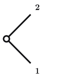
Figure 2: Vertices for the $D_{1}D_{2}$ and $D_{1}^{\dagger}D_{2}^{\dagger}$ operators.

The scalar meson model defined by the lagrangian in Eqs. (4) and (5) can be a low-energy approximation to a more fundamental Lorentz-invariant quantum field theory. If the fundamental quantum field theory includes a high-energy process that can create $D_{1}D_{2}$ with invariant mass near $M_{1+2}$, that process will involve momenta ranging from the highest energy scale to momenta smaller than $m$. If long-distance effects involving momenta much smaller than $m$ can be separated from short-distance effects involving momenta of order $m$ and larger, we can use the scalar meson model to calculate the long-distance effects. Expressions for physical quantities in which short-distance effects and long-distance effects are separated into multiplicative factors are called factorization formulas. The tool required to separate long-distance effects from short-distance effects is the operator product expansion.

III.1 Short-distance production processes

The general production process for $D_{1}D_{2}$ has the form $A\to B+D_{1}D_{2}$, where $A$ and $B$ each represent one or more particles. There can be analogous production processes for $X$. We consider the production of $D_{1}D_{2}$ near their threshold, so that their invariant mass $M$ satisfies the inequality in Eq. (8). We also assume that the relative momentum $\vec{p}\,$ of the $D_{1}$ and $D_{2}$ is small compared to $m$. We call $A\to B+D_{1}D_{2}$ a short-distance production process if all the particles in $A$ and $B$ have momenta in the $D_{1}D_{2}$ rest frame that are of order $m$ or larger. This condition implies that the amplitude for $A\to B+D_{1}D_{2}$ can be expanded in powers of the small energy difference $M-M_{1+2}$ divided by $m^{2}/M_{12}$ and larger energy scales and in powers of the small relative momentum $\vec{p}\,$ divided by $m$ and larger momentum scales. The operator product expansion can be used to express the T-matrix elements in the forms

$${\cal T}[A\to B+D_{1}D_{2}] = \sqrt{4M_{1}M_{2}}\sum_{n}{\cal C}_{A}^{B,n}\,\langle D_{1}D_{2}|{\cal O}_{n}(x=0)|\emptyset\rangle,$$ (20a)

$${\cal T}[A\to B+X] = \sqrt{2M_{X}}\sum_{n}{\cal C}_{A}^{B,n}\,\langle X|{\cal O}_{n}(x=0)|\emptyset\rangle.$$ (20b)

The sums are over local operators ${\cal O}_{n}$ in the effective field theory. They can be restricted to operators with a nonzero matrix element between $\langle D_{1}D_{2}|$ and the vacuum state $|\emptyset\rangle$. The arguments of the operator are the origin $x=0$ of space and time. The operator matrix elements are evaluated in the rest frame of $D_{1}D_{2}$ or $X$. We use the standard nonrelativistic normalizations for the states $\langle D_{1}D_{2}|$ or $\langle X|$ in the operator matrix elements. We use the standard relativistic normalizations for the initial and final states in the T-matrix elements. The factors of $\sqrt{4M_{1}M_{2}}$ and $\sqrt{2M_{X}}$ account for the differences between the normalizations of the states in the operator matrix elements and the T-matrix elements. The Wilson coefficients ${\cal C}_{A}^{B,n}$ in Eq. (20) are functions of the 4-momenta and polarization 4-vectors of the particles in $A$ and $B$ and of the total 4-momentum $P^{\mu}$ of a $D_{1}D_{2}$ pair that is produced exactly at threshold with invariant mass $M_{1+2}$. They also depend on energy scales of order $m^{2}/M_{12}$ and higher and on momentum scales of order $m$ and higher. The only dependence on whether the final state includes $D_{1}D_{2}$ or $X$ is in the operator matrix elements. The leading terms in the expansions of the T-matrix elements in powers of $M-M_{1+2}$ and $\vec{p}\,$ are the terms with the lowest dimension operator $D_{1}^{\dagger}D_{2}^{\dagger}(0)$. In Feynman diagrams, the local operator $D_{1}^{\dagger}D_{2}^{\dagger}$ is represented by an open dot from which a $D_{1}$ line and a $D_{2}$ line emerge, as illustrated in Fig. 2. The Feynman rule for this vertex is 1.

The operator product expansions in Eqs. (20) provide the desired separation of long-distance effects and short-distance effects only if the local operators ${\cal O}_{n}$ are chosen to be renormalized operators that have ultraviolet-finite matrix elements. The simplest local composite operators, such as $D_{1}D_{2}$, generally have matrix elements that are ultraviolet divergent. However the multiplicative renormalizability of local composite operators implies that the relation between the simple local operators ${\cal O}_{n}$ and their renormalized counterparts ${\cal O}^{(R)}_{n}$ can be expressed as

$${\cal O}_{n}(x)=\sum_{m}\left(Z^{-1}\right)_{nm}{\cal O}^{(R)}_{m}(x),$$ (21)

where $Z$ is an infinite-dimensional matrix of renormalization constants. The separation of short-distance effects and long-distance effects in the T-matrix elements in Eqs. (20) is accomplished by making the substitutions in Eq. (21) for the operators ${\cal O}_{n}$. The long-distance factors are matrix elements of the renormalized local operators ${\cal O}^{(R)}_{m}(x=0)$. The short-distance factors are the coefficients of these matrix elements, which are sums of products of Wilson coefficients ${\cal C}_{A}^{B,n}$ and renormalization constants $(Z^{-1})_{nm}$. We will find it more convenient to work with simple composite operators rather than renormalized operators. The combination of the operator product expansion and the multiplicative renormalizability of these operators will be used to separate short-distance effects from long-distance effects.

III.2 Short-distance decay processes

The fundamental theory may also allow transitions $D_{1}D_{2}\to C$ from $D_{1}D_{2}$ with invariant mass $M_{C}$ satisfying $|M_{C}-M_{1+2}|\ll m^{2}/M_{12}$ to a final state $C$ that includes particles other than $D_{1}$ and $D_{2}$. If $M_{C}=M_{X}$, there can be analogous transitions $X\to C$. If the sum of the masses of the particles in $C$ is substantially smaller than $M_{1+2}$, some of the particles in $C$ must emerge with large momenta. We define a short-distance transition to be one for which all the particles in $C$ have momenta in the center-of-momentum frame that are of order $m$ or larger. The T-matrix element for such a process can be expanded in powers of the small energy difference $M_{C}-M_{1+2}$ divided by $m^{2}/M_{12}$ and larger energy scales and in powers of the small relative momentum $\vec{p}\,$ of the $D_{1}$ and $D_{2}$ divided by $m$ and larger momentum scales. The operator product expansion can be used to express the T-matrix elements in the forms

$${\cal T}[D_{1}D_{2}\to C] = \sqrt{4M_{1}M_{2}}\sum_{n}{\cal C}_{n}^{C}\,\langle\emptyset|{\cal O}_{n}(x=0)|D_{1}D_{2}\rangle,$$ (22a)

$${\cal T}[X\to C] = \sqrt{2M_{X}}\sum_{n}{\cal C}_{n}^{C}\,\langle\emptyset|{\cal O}_{n}(x=0)|X\rangle.$$ (22b)

The sums over local operators ${\cal O}_{n}$ of the $D_{1}D_{2}$ model can be restricted to those with a nonzero matrix element between the vacuum $\langle\emptyset|$ and $|D_{1}D_{2}\rangle$. The only dependence on the initial states is in the operator matrix elements. The leading terms in the expansions of the T-matrix elements in powers of $M_{C}-M_{1+2}$ and $\vec{p}\,$ are the terms with the lowest dimension operator $D_{1}D_{2}(0)$. The complete separation of short-distance and long-distance effects is accomplished by using Eq. (21) to eliminate the operators ${\cal O}_{n}$ in favor of renormalized operators.

III.3 Line shape

If the fundamental theory includes short-distance processes that allow the production of $X$ via $A\to B+X$ and the decay of $X$ via $X\to C$, it also allows the process $A\to B+C$, where $C$ represents the same particles but with a variable invariant mass $M_{C}$ instead of $M_{X}$. This process has a resonant enhancement when $M_{C}$ is near the $D_{1}D_{2}$ threshold as specified by Eq. (8). If each of the particles in $A$ and $B$ is well-separated in momentum space from each of the particles in $C$, the T-matrix element for this process can be described within the effective field theory by a double operator product expansion:

$${\cal T}[A\to B+C] = {\cal C}_{A}^{B,C}+\sum_{m,n}{\cal C}_{A}^{B,n}{\cal C}_{m}^{C}\int d^{4}x\,e^{iP\cdot x}\langle\emptyset|{\cal O}_{m}(x){\cal O}_{n}(0)|\emptyset\rangle.$$ (23)

The sum over operators ${\cal O}_{m}$ can be restricted to those with a nonzero matrix element between $\langle D_{1}D_{2}|$ and the vacuum state $|\emptyset\rangle$. The sum over operators ${\cal O}_{n}$ can be restricted to those with a nonzero matrix element between the vacuum $\langle\emptyset|$ and $|D_{1}D_{2}\rangle$. The Wilson coefficients ${\cal C}_{A}^{B,n}$ and ${\cal C}_{m}^{C}$ are the same ones that appear in the operator product expansions in Eqs. (20) and (22). In the Fourier transform of the vacuum–to–vacuum matrix element in Eq. (23), the 4-vector is $P^{\mu}=(M_{C},\vec{0}\,)$. The leading term in the expansion of the T-matrix element in powers of $M_{C}-M_{1+2}$ divided by $m^{2}/M_{12}$ and larger energy scales is the term with the lowest dimension operators $D_{1}D_{2}(x)$ and $D_{1}^{\dagger}D_{2}^{\dagger}(0)$. The first term ${\cal C}_{A}^{B,C}$ on the right side of Eq. (23) takes into account the direct production of $C$ at short distances. This term can be expanded in powers of the small energy difference $M_{C}-M_{1+2}$ divided by $m^{2}/M_{12}$ and larger energy scales. The leading term in the expansion is a constant independent of $M_{C}$. The complete separation of short-distance and long-distance effects is accomplished by using Eq. (21) to eliminate the operators ${\cal O}_{n}$ in favor of renormalized operators.

IV Long-distance processes

In this Section, we give the results for several quantities in the scalar meson model that depend only on long distances: the Green’s function for $D_{1}D_{2}\to D_{1}D_{2}$, the cross section for elastic $D_{1}D_{2}$ scattering, and the propagator for the bound state $X$.

IV.1 Green’s function for $D_{1}D_{2}\to D_{1}D_{2}$

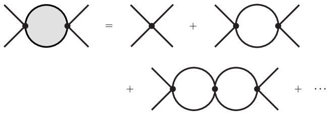
Figure 3: The amputated connected Green’s function $i{\cal A}_{0}(E)$ for $D_{1}D_{2}\to D_{1}D_{2}$ at $0^{\textrm{th}}$ order in $g$. It can be obtained by summing a geometric series of diagrams.

In the scalar meson model, all the observables for processes near the $D_{1}D_{2}$ threshold are related in a simple way to the Green’s function for $D_{1}D_{2}\to D_{1}D_{2}$. We denote the amputated connected Green’s function for $D_{1}D_{2}\to D_{1}D_{2}$ by $i{\cal A}_{0}(E)$, because it depends only on the total energy $E$ in the $D_{1}D_{2}$ rest frame. It can be calculated nonperturbatively by summing the geometric series represented by Fig. 3 to all orders in $\lambda_{0}$:

$$i{\cal A}_{0}(E)=\frac{-i}{1/\lambda_{0}-L_{0}(E)},$$ (24)

where $iL_{0}(E)$ is the amplitude for the propagation of the $D_{1}D_{2}$ pair between successive contact interactions. The function $L_{0}(E)$ has an ultraviolet divergence that can be isolated into an additive term that is independent of $E$. It can be expressed as

$$L_{0}(E)=L_{0}(M_{1+2})+\frac{M_{12}}{2\pi}\sqrt{-2M_{12}E_{12}-i\varepsilon},$$ (25)

where $E_{12}$ is the energy relative to the $D_{1}D_{2}$ threshold:

$$E_{12} = E-M_{1+2}.$$ (26)

The ultraviolet divergence is contained in the term $L_{0}(M_{1+2})$. If we use an ultraviolet momentum cutoff $\Lambda\gg|M_{12}E_{12}|^{1/2}$, this term has a linear ultraviolet divergence: $L_{0}(M_{1+2})=-(M_{12}/\pi^{2})\Lambda$. If we use dimensional regularization, this term is $L_{0}(M_{1+2})=0$, because dimensional regularization sets power ultraviolet divergences equal to 0.

One can identify the combination $1/\lambda_{0}-L_{0}(M_{1+2})$ on the right side of Eq. (24) as a renormalized inverse coupling constant $1/\lambda$. One possible renormalization prescription is to eliminate $1/\lambda_{0}$ in favor of $1/\lambda$. Another possible renormalization prescription is to eliminate $\lambda_{0}$ in favor of the scattering length $a$ defined in Eq. (9). The most convenient renormalization prescription for our purposes is to demand that the pole in the amplitude ${\cal A}_{0}(E)$ be at the energy $E_{\rm pole}$ given in Eq. (10). Inserting the expression for $L_{0}(E)$ in Eq. (25) into the amplitude in Eq. (24) and eliminating $\lambda_{0}$ in favor of $\gamma$, the amplitude reduces to

$${\cal A}_{0}(E)=\frac{2\pi/M_{12}}{-\gamma+\sqrt{-2M_{12}E_{12}-i\varepsilon}}.$$ (27)

The renormalized expression for the amplitude ${\cal A}_{0}(E)$ in Eq. (27) follows from the renormalization prescription in Eq. (10) and is independent of the regularization scheme. The expression for the bare coupling constant is

$$\lambda_{0}=\frac{1}{L_{0}(M_{1+2})+M_{12}(\gamma_{\rm re}+i\gamma_{\rm im})/(2\pi)}.$$ (28)

With dimensional regularization, $L_{0}(M_{1+2})=0$, so Eq. (28) gives a finite relation between $\lambda_{0}$ and the binding momentum $\gamma$: $\lambda_{0}=2\pi/(M_{12}\gamma)$. We will see later that that the naive use of dimensional regularization can be misleading.

IV.2 Elastic $D_{1}D_{2}$ Scattering

We can use the amplitude in Eq. (27) to determine the T-matrix element for the elastic scattering of $D_{1}$ and $D_{2}$ with relative momentum $p$. In the $D_{1}D_{2}$ center-of-momentum frame, the total energy of the $D_{1}$ and $D_{2}$ is

$$E_{\rm cm}(p)=M_{1+2}+p^{2}/(2M_{12}).$$ (29)

The energy variable $E_{12}$ defined in Eq. (26) reduces to $E_{12}=p^{2}/(2M_{12})$. The T-matrix element is obtained by evaluating the amplitude ${\cal A}_{0}(E)$ in Eq. (27) at the energy $E_{\rm cm}(p)$ in Eq. (29) and multiplying by the factor $4M_{1}M_{2}$ to account for the relativistic normalization of states:

$${\cal T}_{12\to 12}(p)=-\frac{8\pi M_{1+2}}{\gamma+ip}.$$ (30)

The complex $D_{1}D_{2}$ scattering length defined by Eq. (9) is therefore simply

$$a=1/(\gamma_{\rm re}+i\gamma_{\rm im}).$$ (31)

We obtain the cross section for elastic $D_{1}D_{2}$ scattering by squaring the T-matrix element, integrating over the phase space of the $D_{1}$ and $D_{2}$ in the final state, and multiplying by a flux factor. The energy $E_{\rm cm}(p)$ in the $D_{1}D_{2}$ rest frame is assumed to be close to $M_{1+2}$, as specified by the condition in Eq. (8). The product of the phase space factor $\lambda^{1/2}(E_{\rm cm}(p),M_{1},M_{2})/(8\pi M_{1+2}^{2})$ and the flux factor $1/(4M_{1+2}p)$ can therefore be approximated by $1/(16\pi M_{1+2}^{2})$. The cross section is

$$\sigma[D_{1}D_{2}(\vec{p}\,)\to D_{1}D_{2}]=\frac{4\pi}{|\gamma_{\rm re}+i(\gamma_{\rm im}+p)|^{2}}.$$ (32)

The argument $(\vec{p}\,)$ of $D_{1}D_{2}$ in the initial state implies that the $D_{1}$ and $D_{2}$ have momenta $-\vec{p}\,$ and $+\vec{p}\,$, respectively. The momenta of the $D_{1}$ and $D_{2}$ in the final state are not specified because they have been integrated over.

IV.3 Propagator for $X$

If the local composite operator $D_{1}D_{2}(x)$ is used as an interpolating field for $X$, the propagator for $X$ is given in Eq. (16). The diagrams for the propagator of $X$ are shown in Fig. 5. In the rest frame $P=0$, these diagrams form a geometric series whose sum is

$$i\Delta_{X}(E,0)=\frac{iL_{0}(E)}{1-\lambda_{0}L_{0}(E)}.$$ (33)

This propagator has a pole in $E$ at the same energy $E_{\rm pole}$ given in Eq. (10) as the amplitude ${\cal A}_{0}(E)$ in Eq. (24). Near the pole, the behavior of the propagator at $P=0$ is given in Eq. (17). Using $L_{0}(E_{\rm pole})=1/\lambda_{0}$, we determine the wavefunction normalization factor to be

$$Z_{X}=\frac{2\pi\gamma}{M_{12}^{2}\lambda_{0}^{2}}.$$ (34)

Using the expression for ${\cal A}_{0}(E)$ in Eq. (24), the propagator for $X$ in Eq. (33) can be expressed as

$$\Delta_{X}(E,0)=-{\cal A}_{0}(E)\frac{L_{0}(E)}{\lambda_{0}}.$$ (35)

The alternative expression for ${\cal A}_{0}(E)$ in Eq. (27) shows that, after renormalization of the coupling constant, it does not depend on the ultraviolet cutoff $\Lambda$. Thus the propagator in Eq. (35) depends on $\Lambda$ only through the factor $L_{0}(E)/\lambda_{0}$. That there is some dependence on $\Lambda$ is not a surprise, because we have used the simple composite operator $D_{1}D_{2}(x)$ as the interpolating field for $X$ rather than a renormalized operator. As we shall see in Sec. V, $\lambda_{0}D_{1}D_{2}(x)$ is a renormalized operator whose matrix elements between the vacuum $\langle\emptyset|$ and $|D_{1}D_{2}\rangle$ or $|X\rangle$ do not depend on the ultraviolet cutoff. The propagator for the renormalized operator $\lambda_{0}D_{1}D_{2}(x)$ is obtained by multiplying the expression in Eq. (35) by $\lambda_{0}^{2}$. But this propagator depends on $\Lambda$ through the factor $\lambda_{0}L_{0}(E)$. To obtain a renormalized propagator that does not depend on $\Lambda$, one must add the $\Lambda$-dependent constant $i\lambda_{0}$ to the propagator for the renormalized operator $\lambda_{0}D_{1}D_{2}(x)$:

$$i\lambda_{0}^{2}\,\Delta_{X}(E,0)+i\lambda_{0}=-i{\cal A}_{0}(E)~{}.$$ (36)

Thus the renormalized propagator is essentially just the amplitude ${\cal A}_{0}(E)$ in Eq. (27). The need for adding the constant term in Eq. (36) is related to the fact that if an external source coupled to a composite operator is added to the lagrangian, renormalization sometimes requires the addition of terms with higher powers of the source Zinn-Justin . For example, the addition of the term $J^{\dagger}D_{1}D_{2}+{\rm h.c.}$ creates new ultraviolet divergences that can only be cancelled by a $J^{\dagger}J$ term. Such a term is required even in the absence of any interactions. To implement the LSZ prescription for T-matrix elements for processes with $X$ in the initial or final state, it is not necessary to use a renormalized propagator. We will use the unrenormalized propagator for $X$ in Eq. (35) for this purpose.

V Short-distance processes

In this Section, we consider processes in the scalar meson model that involve both short-distance and long-distance effects: short-distance production rates, short-distance decay rates, and the line shape of the bound state in a short-distance decay mode. We use the operator product expansion to derive factorization formulas in which those short-distance effects and long-distance effects are separated. After renormalization of the coupling constant, all remaining depedence on the ultraviolet cutoff can be removed by renormalization of the Wilson coefficients in the operator product expansion.

V.1 Short-distance Production of $X$ and $D_{1}D_{2}$

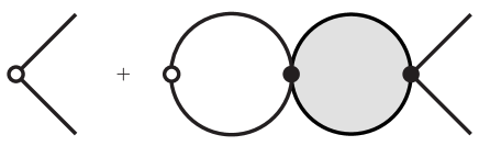
Figure 4: Diagrams at 0^th order in $g$ for the vacuum–to–$D_{1}D_{2}$ matrix element of the operator $D_{1}^{\dagger}D_{2}^{\dagger}$.

We consider the short-distance production processes $A\to B+D_{1}D_{2}$ and $A\to B+X$, where $A$ and $B$ both represent one or more particles whose momenta in the $D_{1}D_{2}$ or $X$ rest frame are all of order $m$ or larger. The operator product expansions of the T-matrix element for such short-distance processes are given in Eqs. (20). The leading terms in the expansions are the ones with the local operator $D_{1}^{\dagger}D_{2}^{\dagger}(0)$. If we keep only these leading terms, the Lorentz-invariant T-matrix elements reduce to

$${\cal T}[A\to B+D_{1}D_{2}] = \sqrt{4M_{1}M_{2}}\,{\cal C}_{A}^{B,12}\,\langle D_{1}D_{2}|D_{1}^{\dagger}D_{2}^{\dagger}(0)|\emptyset\rangle,$$ (37a)

$${\cal T}[A\to B+X] = \sqrt{2M_{X}}\,{\cal C}_{A}^{B,12}\,\langle X|D_{1}^{\dagger}D_{2}^{\dagger}(0)|\emptyset\rangle.$$ (37b)

We first consider the T-matrix element for the production of $D_{2}D_{2}$ via the short-distance process $A\to B+D_{1}D_{2}$. We take the $D_{1}$ and $D_{2}$ in Eq. (37a) to have relative momentum $\vec{p}\,$ in the $D_{1}D_{2}$ rest frame and unspecified total momentum. Their invariant mass is $M=E_{\rm cm}(p)$, where $E_{\rm cm}(p)$ is given in Eq. (29). This invariant mass is assumed to be close to $M_{1+2}$, as specified by the inequality in Eq. (8). The Feynman diagrams for the vacuum–to–$D_{1}D_{2}$ matrix element, which are shown in Fig. 4, form a geometric series. The matrix element in Eq. (37a) is therefore

$$\langle D_{1}D_{2}(\vec{p}\,)|D_{1}^{\dagger}D_{2}^{\dagger}(0)|\emptyset\rangle=\frac{1}{1-\lambda_{0}L_{0}(E_{\rm cm}(p))}.$$ (38)

The argument $(\vec{p}\,)$ of the $D_{1}D_{2}$ state implies that the $D_{1}$ and $D_{2}$ have momenta $-\vec{p}\,$ and $+\vec{p}\,$, respectively. The sum of the diagrams in Fig. 4 differs from the geometric series of diagrams for $i{\cal A}_{0}(E)$ in Fig. 3 only by the multiplicative factor $1/(-i\lambda_{0})$. Since ${\cal A}_{0}(E)$, which after renormalization of the coupling constant is given by Eq. (27), does not depend on the ultraviolet cutoff, the operator $\lambda_{0}D_{1}^{\dagger}D_{2}^{\dagger}(x)$ is a renormalized operator whose matrix elements do not depend on the ultraviolet cutoff. The T-matrix element in Eq. (37a) can be separated into a short-distance factor and a long-distance factor by taking the long-distance factor to be the matrix element of the renormalized operator:

$${\cal T}[A\to B+D_{1}D_{2}(\vec{p}\,)]=-\sqrt{4M_{1}M_{2}}\,\big{(}{\cal C}_{A}^{B,12}/\lambda_{0}\big{)}\,{\cal A}_{0}(E_{\rm cm}(p)).$$ (39)

After renormalization of the coupling constant, ${\cal A}_{0}(E_{\rm cm}(p))$ is given by the expression in Eq. (27), which does not depend on the ultraviolet cutoff $\Lambda$. The T-matrix element in Eq. (39) will not depend on $\Lambda$ if the short-distance factor ${\cal C}_{A}^{B,12}/\lambda_{0}$ does not depend on $\Lambda$. Equivalently, the dependence on $\Lambda$ can be removed by a multiplicative renormalization of the Wilson coefficient ${\cal C}_{A}^{B,12}$.

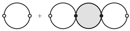
Figure 5: Feynman diagrams for the $X$ propagator at 0^th order in $g$. The interpolating field for the $X$ is $D_{1}D_{2}(x)$.

We next consider the T-matrix element for the production of $X$ via the short-distance process $A\to B+X$. The operator product expansion of the T-matrix element for this process is given in Eq. (37b). The vacuum–to–$X$ matrix element can be obtained via the LSZ formalism from the connected Green’s function for the operator $D_{1}^{\dagger}D_{2}^{\dagger}$ that acts on the vacuum and an operator $D_{1}D_{2}$ associated with the $X$ in the final state. This connected Green’s function is identical to the propagator $i\Delta_{X}(E,0)$ given in Eq. (33). The matrix element in Eq. (37b) is the normalized on-shell amputated connected Green’s function. The Green’s function is amputated by multiplying by the inverse propagator $[i\Delta_{X}(E,0)]^{-1}$, which simply gives 1. In the rest frame of $X$ where its momentum is $\vec{P}\,=0$, the Green’s function is put on shell by setting the energy $E$ equal to the energy $E_{\rm pole}$ in Eq. (10), although the absence of any dependence on $E$ makes this condition moot. Finally the Green’s function is normalized by multiplying by the factor $Z_{X}^{1/2}$, where $Z_{X}$ is given in Eq. (34). Thus the vacuum–to–$X$ matrix element is simply

$$\langle X|D_{1}^{\dagger}D_{2}^{\dagger}(0)|\emptyset\rangle=\frac{(2\pi\gamma)^{1/2}}{M_{12}\lambda_{0}}.$$ (40)

The only factors in the T-matrix element in Eq. (37b) that are sensitive to short distances are the Wilson coefficient ${\cal C}_{A}^{B,12}$ and the factor of $1/\lambda_{0}$ from the matrix element. The T-matrix element in Eq. (37b) can be expressed as the product of a short-distance factor and a long-distance factor:

$${\cal T}[A\to B+X]=\sqrt{2M_{X}}\,\big{(}{\cal C}_{A}^{B,12}/\lambda_{0}\big{)}\,\frac{(2\pi\gamma)^{1/2}}{M_{12}}.$$ (41)

The short-distance factor ${\cal C}_{A}^{B,12}/\lambda_{0}$ is the same one that appears in Eq. (39).

The factored expressions for the T-matrix elements in Eqs. (39) and (41) lead to factored expressions for the production rates. The rates for producing $X$ and $D_{1}D_{2}$ are obtained by squaring the amplitudes and integrating over the appropriate phase space. If $A$ consists of a single particle, the decay rate into $B+X$ can be expressed in the factored form

$$\Gamma[A\to B+X]=\Gamma_{A}^{B}\,\frac{2\pi}{M_{12}}\left|\gamma_{\rm re}^{2}+\gamma_{\rm im}^{2}\right|^{1/2},$$ (42)

where $\Gamma_{A}^{B}$ is a short-distance factor with dimensions of mass:

$$\Gamma_{A}^{B} = \frac{M_{1+2}}{M_{A}M_{12}}\int\frac{d^{3}P_{1+2}}{(2\pi)^{3}2E_{1+2}}\int\prod_{i\in B}\frac{d^{3}p_{i}}{(2\pi)^{3}2E_{i}}\left|{\cal C}_{A}^{B,12}/\lambda_{0}\right|^{2}(2\pi)^{4}\delta^{(4)}(P_{A}^{\mu}-P_{1+2}^{\mu}-\mbox{$\sum\limits_{i\in B}$}\,p_{i}^{\mu}).$$

The 4-momentum $P_{1+2}^{\mu}$ is that of a $D_{1}D_{2}$ pair exactly at threshold with invariant mass $M_{1+2}$. We have chosen the long-distance factor in Eq. (42) to be the square of the long-distance factor in the T-matrix element in Eq. (41) multiplied by $M_{12}$ to make it dimensionless. All factors from integrating over the phase space of the particles in the final state are included in the short-distance factor. The differential rate for producing $D_{1}D_{2}$ with invariant mass $M=E_{\rm cm}(p)$ given by Eq. (29) can be expressed in the factored form

$$\frac{d\Gamma}{dM}[A\to B+D_{1}D_{2}(\vec{p}\,)]=\Gamma_{A}^{B}\,\frac{2p}{|\gamma_{\rm re}+i(\gamma_{\rm im}+p)|^{2}}.$$ (44)

The short-distance factor $\Gamma_{A}^{B}$ is the same as in Eq. (42). The long-distance factor is the product of $4M_{1}M_{2}|{\cal A}_{0}(E_{\rm cm}(p))|^{2}$ from the T-matrix element in Eq. (39), the phase space factor $\lambda^{1/2}(E_{\rm cm}(p),M_{1},M_{2})/(8\pi E_{\rm cm}(p)^{2})$, the kinematic factor $E_{\rm cm}(p)/\pi$ associated with the differential $dM$, and a factor $M_{12}/(2M_{1+2})$ to compensate for the choice of prefactor in Eq. (LABEL:GamADDB-scalar). Using the expression for the invariant mass $E_{\rm cm}(p)$ in Eq. (29) and replacing $E_{\rm cm}(p)$ by $M_{1+2}$ in every factor that is insensitive to $p$, the product of the phase space and kinematic factors can be reduced to $p/(4\pi^{2})$.

V.2 Short-distance Decay of $X$

The fundamental theory may have short-distance processes though which $X$ can decay. We consider the short-distance decay process $X\to C$, where $C$ represents two or more particles whose momenta in the $X$ rest frame are of order $m$ or larger. The operator product expansion for this decay process is given in Eq. (22b). The leading term in the expansion is the one with the operator $D_{1}D_{2}(x)$. If we keep only this term, the T-matrix element reduces to

$${\cal T}[X\to C]=\sqrt{2M_{X}}\,{\cal C}_{12}^{C}\,\langle\emptyset|D_{1}D_{2}(0)|X\rangle.$$ (45)

The $X$–to–vacuum matrix element can be calculated in a similar way to the vacuum–to–$X$ matrix element in Eq. (40):

$$\langle\emptyset|D_{1}D_{2}(0)|X\rangle=\frac{(2\pi\gamma)^{1/2}}{M_{12}\lambda_{0}}.$$ (46)

This matrix element depends on the ultraviolet cutoff only through the factor $1/\lambda_{0}$. In the T-matrix element in Eq. (45), the separation of short-distance and long-distance effects can be accomplished by taking the long-distance factor to be the matrix element of the renormalized operator $\lambda_{0}D_{1}D_{2}(0)$:

$${\cal T}[X\to C]=\sqrt{2M_{X}}\,\big{(}{\cal C}_{12}^{C}/\lambda_{0}\big{)}\,\frac{(2\pi\gamma)^{1/2}}{M_{12}}.$$ (47)

This T-matrix element will not depend on the ultraviolet cutoff $\Lambda$ if the short-distance factor ${\cal C}_{12}^{C}/\lambda_{0}$ does not depend on $\Lambda$. Equivalently, the dependence on $\Lambda$ can be removed by a multiplicative renormalization of the Wilson coefficient ${\cal C}_{12}^{C}$.

The decay rate of $X$ into the particles represented by $C$ is obtained by squaring the T-matrix element and integrating over the phase space of those particles. It can be expressed in the factored form

$$\Gamma[X\to C]=\Gamma^{C}\;\frac{2\pi}{M_{12}}\left|\gamma_{\rm re}^{2}+\gamma_{\rm im}^{2}\right|^{1/2},$$ (48)

where $\Gamma^{C}$ is a short-distance factor with dimensions of mass:

$$\Gamma_{C}=\frac{1}{M_{12}}\int\prod_{j\in C}\frac{d^{3}p_{j}}{(2\pi)^{3}2E_{j}}\left|{\cal C}^{C}_{12}/\lambda_{0}\right|^{2}(2\pi)^{4}\delta^{(4)}\!(P_{1+2}^{\mu}-\mbox{$\sum\limits_{j\in C}$}p_{j}^{\mu}).$$ (49)

We have chosen the long-distance factor to be the square of the long-distance factor in the T-matrix element in Eq. (47) multiplied by $M_{12}$ to make it dimensionless.

The separation of short-distance and long-distance effects for the transition $D_{1}(-\vec{p}\,)D_{2}(\vec{p}\,)\to C$ can be accomplished in a similar way. The operator product expansion for the T-matrix element is given in Eq. (22a). The T-matrix element can be expressed as the product of the same short-distance factor as in Eq. (47) and a long-distance factor that includes a factor of ${\cal A}_{0}(E_{\rm cm}(p))$, where $E_{\rm cm}(p)$ is the energy in Eq. (29).

V.3 Line shape of $X$ in a Short-distance Decay Mode

If the fundamental theory includes short-distance processes that allow the production of $X$ via $A\to B+X$ and the decay of $X$ via $X\to C$, it also allows the process $A\to B+C$, where $C$ represents the same particles but with a variable invariant mass $M_{C}$ instead of $M_{X}$. We assume that $M_{C}$ is near the $D_{1}D_{2}$ threshold as specified by Eq. (8). If every particle in $A$ and $B$ has momentum in the rest frame of $C$ of order $m$ or larger, the T-matrix element for this process can be expressed as the double operator product expansion in Eq. (23). The Wilson coefficient $C_{A}^{B,C}$ can be expanded in powers of $M_{C}-M_{1+2}$ divided by $m^{2}/M_{12}$ and higher energy scales. The leading term in this expansion is simply a constant independent of $M_{C}$. The leading terms in the double sum come from the operators ${\cal O}_{n}(0)=D_{1}^{\dagger}D_{2}^{\dagger}(0)$ and ${\cal O}_{m}(x)=D_{1}D_{2}(x)$. According to Eq. (16), the Fourier transform of the matrix element of these operators in the $C$ rest frame is just the $X$ propagator, which is given in Eq. (33) or (35), evaluated at $E=M_{C}$. Thus the T-matrix element reduces to

$${\cal T}[A\to B+C] = {\cal C}_{A}^{B,C}+{\cal C}_{A}^{B,12}{\cal C}_{12}^{C}\frac{iL_{0}(M_{C})}{1-\lambda_{0}L_{0}(M_{C})}.$$ (50)

The Wilson coefficients and the factor $L_{0}(E)/\lambda_{0}$ in the $X$ propagator depend on the ultraviolet cutoff $\Lambda$. All the dependence on the energy can be isolated in a term that does not depend on $\Lambda$ by using the fact that the combination in Eq. (36) does not depend on $\Lambda$. By subtracting and adding $i{\cal C}_{A}^{B,12}{\cal C}_{12}^{C}/\lambda_{0}$ to the two terms on the right side of Eq. (50), the T-matrix element can be expressed as

$${\cal T}[A\to B+C] = \big{(}{\cal C}_{A}^{B,C}-i{\cal C}_{A}^{B,12}{\cal C}_{12}^{C}/\lambda_{0}\big{)}-i\big{(}{\cal C}_{A}^{B,12}/\lambda_{0}\big{)}\big{(}{\cal C}_{12}^{C}/\lambda_{0}\big{)}\,{\cal A}_{0}(M_{C}).$$ (51)

After renormalization of the coupling constant, ${\cal A}_{0}(E)$ is given in Eq. (27). The short-distance factors ${\cal C}_{A}^{B,12}/\lambda_{0}$ and ${\cal C}_{12}^{C}/\lambda_{0}$ in Eq. (51) cannot depend on $\Lambda$, because otherwise the T-matrix elements in Eqs. (39), (41), and (47) would depend on $\Lambda$. Thus the T-matrix element in Eq. (51) will not depend on $\Lambda$ if the constant term ${\cal C}_{A}^{B,C}-i{\cal C}_{A}^{B,12}{\cal C}_{12}^{C}/\lambda_{0}$ does not depend on $\Lambda$. Equivalently, the dependence on $\Lambda$ can be removed by an additive renormalization of the Wilson coefficient ${\cal C}_{A}^{B,C}$. It is convenient to express the T-matrix element in Eq. (51) in the form

$${\cal T}[A\to B+C] = -i\big{(}{\cal C}_{A}^{B,12}/\lambda_{0}\big{)}\big{(}{\cal C}_{12}^{C}/\lambda_{0}\big{)}\left[{\cal A}_{0}(M_{C})-(2\pi/M_{12})c_{A}^{B,C}\right],$$ (52)

where $c_{A}^{B,C}$ is a complex constant with dimension of length that is completely determined by short-distance factors. The natural scale for $c_{A}^{B,C}$ is $1/m$, where $m$ is the mass of the lightest meson that can be exchanged between $D_{1}$ and $D_{2}$.

The factored expression for the T-matrix element in Eq. (52) leads to a factored expression for the rate for $A\to B+C$. The invariant mass distribution of the particles in $C$ is obtained by squaring the T-matrix element and integrating over the momenta of all the particles in the final state. It is convenient to express the phase space integral in an iterated form corresponding to the production of the particles in $B$ and an effective particle of mass $M_{C}$ followed by the decay of that effective particle into the particles in $C$. If $A$ is a single particle, the decay rate is

$$\Gamma[A\to B+C] = \frac{1}{2M_{A}}\int\frac{dM_{C}^{2}}{2\pi}\int\frac{d^{3}P_{C}}{(2\pi)^{3}2E_{C}}\int\prod_{i\in B}\frac{d^{3}p_{i}}{(2\pi)^{3}2E_{i}}(2\pi)^{4}\delta^{(4)}(P_{A}^{\mu}-P_{C}^{\mu}-\mbox{$\sum\limits_{i\in B}$}p_{i}^{\mu})$$ (53)

$$\times\int\prod_{j\in C}\!\frac{d^{3}p_{j}}{(2\pi)^{3}2E_{j}}(2\pi)^{4}\delta^{(4)}(P_{C}^{\mu}-\mbox{$\sum\limits_{j\in C}$}p_{j}^{\mu})\left|{\cal T}[A\to B+C]\right|^{2}.$$

The invariant mass $M_{C}$ of the particles in $C$ can be replaced by $M_{1+2}$ everywhere except in the long-distance factor of the T-matrix element. In that long-distance factor, it can be expressed as

$$M_{C}=M_{1+2}+p_{C}^{2}/(2M_{12}),$$ (54)

where $p_{C}^{2}$ can be positive or negative. The variable $p_{C}$ is pure imaginary if $M_{C}<M_{1+2}$ and real and positive if $M_{C}>M_{1+2}$. The differential decay rate of the particle $A$ for $M_{C}$ near $M_{1+2}$ reduces to

$$\frac{d\Gamma}{dM_{C}}[A\to B+C] = \big{(}\Gamma_{A}^{B}\Gamma^{C}\big{)}\,2\pi\left|\frac{1}{(\gamma_{\rm re}-|p_{C}|)+i\gamma_{\rm im}}+c_{A}^{B,C}\right|^{2}\hskip 19.91684ptM_{C}<M_{1+2},$$ (55a)

$$= \big{(}\Gamma_{A}^{B}\Gamma^{C}\big{)}\,2\pi\left|\frac{1}{\gamma_{\rm re}+i(\gamma_{\rm im}+p_{C})}+c_{A}^{B,C}\right|^{2}\hskip 28.45274ptM_{C}>M_{1+2}.$$ (55b)

The short-distance factors $\Gamma_{A}^{B}$ and $\Gamma^{C}$ are the same as in Eqs. (42), (44), and (48). All other short-distance effects are contained in the complex constant $c_{A}^{B,C}$. The invariant mass distribution in Eq. (55) is continuous at $M_{C}=M_{1+2}$.

The separation of scales represented by the renormalized operator product expansions for the T-matrix elements in Eqs. (39), (41), (47), and (51) can be obscured by using dimensional regularization. In a generic regularization scheme with ultraviolet cutoff $\Lambda$, the short-distance quantities $\lambda_{0}$, ${\cal C}_{A}^{B,12}$, ${\cal C}_{12}^{C}$, and ${\cal C}_{A}^{B,C}$ are insensitive to $\gamma$. They depend on $\Lambda$ in such a way that the combinations ${\cal C}_{A}^{B,12}/\lambda_{0}$, ${\cal C}_{12}^{C}/\lambda_{0}$, and ${\cal C}_{A}^{B,C}-i{\cal C}_{A}^{B,12}{\cal C}_{12}^{C}/\lambda_{0}$ do not depend on $\Lambda$. Dimensional regularization sets power ultraviolet divergences to zero. In particular, it sets $L_{0}(M_{1+2})=0$, so the expression for the bare coupling constant in Eq. (28) reduces to $\lambda_{0}=2\pi/(M_{12}\gamma)$. The Wilson coefficients ${\cal C}_{A}^{B,12}$, ${\cal C}_{12}^{C}$, and ${\cal C}_{A}^{B,C}$ do not depend on the ultraviolet cutoff of dimensional regularization. Compatibility with other regularization schemes requires however that they depend on $\gamma$ in such a way that the combinations ${\cal C}_{A}^{B,12}/\lambda_{0}$, ${\cal C}_{12}^{C}/\lambda_{0}$, and ${\cal C}_{A}^{B,C}-i{\cal C}_{A}^{B,12}{\cal C}_{12}^{C}/\lambda_{0}$ are insensitive to $\gamma$. This requires that ${\cal C}_{A}^{B,12}$ and ${\cal C}_{12}^{C}$ have multiplicative factors of $\gamma^{-1}$ and that ${\cal C}_{A}^{B,C}$ have an additive term with a factor $\gamma^{-1}$. Thus the Wilson coefficients in dimensional regularization are not short-distance factors. Their dependence on $\gamma$ is similar to the dependence of the Wilson coefficients on $\Lambda$ in other regularization schemes. That dependence cancels in the combinations of Wilson coefficients and $\lambda_{0}$ that appear in the renormalized operator product expansions for the T-matrix elements.

VI Large scattering length expansion

Effective field theories can exploit a large separation of momentum scales by providing a simpler description of the lowest momentum scale. Another important feature of effective field theories is that they provide a systematic framework for improving the accuracy of the description to any desired order in the ratio of the small momentum scale and higher momentum scales. In this Section, we discuss how the accuracy of the results for the scalar meson model in Secs. IV and V can be systematically improved using an expansion in the large scattering length. We also explain how that expansion can be exploited to simplify some of the results in Sec. V.

In the scalar meson model, the smallest momentum scale is the scale $|\gamma|$ associated with the large scattering length. In a more fundamental theory, there may be many larger momentum scales, but the most important at low energies is the mass $m$ of the lightest meson that can be exchanged between $D_{1}$ and $D_{2}$. The model defined by the lagrangian in Eqs. (4) and (5) reproduces all effects that are not suppressed by powers of $|\gamma|/m$. The model can be systematically improved so that it reproduces all corrections to any desired order in $|\gamma|/m$. We will discuss only the improvements required to reproduce corrections through first order in $|\gamma|/m$.

The only improvement in the effective theory that is required to decrease the errors to second order in $|\gamma|/m$ is to take into account the effective range $r_{s}$ for S-wave scattering. This parameter can be defined by the low-momentum expansion for the inverse of the T-matrix element:

$$\frac{1}{{\cal T}(p)} = -\frac{1}{8\pi M_{1+2}}\left(\frac{1}{a}+ip-\frac{1}{2}r_{s}p^{2}+\cdots\right)~{}.$$ (56)

If we impose the renormalization condition that the Green’s function for $D_{1}D_{2}\longrightarrow D_{1}D_{2}$ has a pole at the energy $E_{\rm pole}$ given in Eq. (10), one expression that will give the correct effective range is

$${\cal A}(E) = \frac{-2\pi/M_{12}}{(\gamma+ip)[1-r_{s}(\gamma-ip)/2]}~{},$$ (57)

where $p=i\sqrt{-2M_{12}E_{12}-i\varepsilon}$. The corresponding T-matrix element for elastic $D_{1}D_{2}$ scattering is then

$${\cal T}_{12\to 12}(p)=\frac{-8\pi M_{1+2}}{(\gamma+ip)[1-r_{s}(\gamma-ip)/2]}.$$ (58)

In short-distance observables, there are additional terms in the expansions in $|\gamma|/m$ coming from higher dimension operators in the operator product expansion. For each additional gradient in the operator, the operator matrix element will have an additional factor of order $\gamma$. The dimensions from these additional factors of $\gamma$ must be compensated by factors of $1/m$ in the short-distance coefficients. Only operators with a single gradient can give contributions that are suppressed by one power of $|\gamma|/m$. The matrix element of the operator $\nabla^{i}(D_{1}D_{2})$ between $|D_{1}D_{2}(\vec{p}\,)\rangle$ or $|X\rangle$ and the vacuum $\langle\emptyset|$ vanishes in the center-of-momentum frame. The other independent operator with a single gradient is $\nabla^{i}D_{1}D_{2}-D_{1}\nabla^{i}D_{2}$. The matrix element $\langle\emptyset|\nabla^{i}D_{1}D_{2}-D_{1}\nabla^{i}D_{2}|X\rangle$ must vanish because the operator is a vector and there are no vectors associated with the state $|X\rangle$ in its center-of-mass frame. The matrix element $\langle\emptyset|\nabla^{i}D_{1}D_{2}-D_{1}\nabla^{i}D_{2}|D_{1}D_{2}(\vec{p}\,)\rangle$ is nonzero and proportional to $p^{i}$. This operator gives a term in the T-matrix element for $A\to B+D_{1}D_{2}(\vec{p}\,)$ in Eq. (39) that is linear in the momentum $\vec{p}\,$ but has a suppression factor of $1/m$ in the short-distance coefficient. Higher dimension operators in the operator product expansion will contribute to the T-matrix elements for $A\to B+X$ in Eq. (41), for $X\to C$ in Eq. (47), and for $A\to B+C$ in Eq. (52) only at second and higher orders in $|\gamma|/m$.

The systematic expansion in powers of $|\gamma|/m$ can be used to simplify the leading order results for short-distance observables. The T-matrix element for $A\to B+C$ in Eq. (52) has a resonant term ${\cal A}_{0}(M_{C})$ and a nonresonant term $c_{A}^{B,C}$. The resonant term ${\cal A}_{0}(M_{C})$ includes a factor that is of order $1/|\gamma|$ when $p_{C}$ is of order $|\gamma|$. The nonresonant term $c_{A}^{B,C}$ is completely determined by short-distance effects, so the natural scale for $c_{A}^{B,C}$ is $1/m$. For $p_{C}$ of order $|\gamma|$, this amplitude is suppressed by $|\gamma|/m$ compared to the resonant term in Eq. (52). One can therefore set $c_{A}^{B,C}=0$ by truncating the expansion at leading order in $|\gamma|/m$. The invariant mass distribution in Eq. (55) then reduces to

$$\frac{d\Gamma}{dM_{C}}[A\to B+C] = \big{(}\Gamma_{A}^{B}\Gamma^{C}\big{)}\,\frac{2\pi}{(\gamma_{\rm re}-|p_{C}|)^{2}+\gamma_{\rm im}^{2}}\hskip 19.91684ptM_{C}<M_{1+2},$$ (59a)

$$= \big{(}\Gamma_{A}^{B}\Gamma^{C}\big{)}\,\frac{2\pi}{\gamma_{\rm re}^{2}+(\gamma_{\rm im}+p_{C})^{2}}\hskip 28.45274ptM_{C}>M_{1+2}.$$ (59b)

This simple factorization formula was first derived in Ref. Braaten:2005jj . If the nonresonant amplitude $c_{A}^{B,C}$ in Eq. (55) is included, the systematic expansion in powers of $|\gamma|/m$ requires that all other terms that are first order in $|\gamma|/m$ also be included. This requires that the effective field theory be improved so that it takes into account the effective range.

The above derivation of the simple factorization formula in Eq. (59) is much cleaner than the derivation in Ref. Braaten:2005jj . In Ref. Braaten:2005jj , the authors used an ultraviolet momentum cutoff $\Lambda$. They obtained results that did not depend on $\Lambda$ by taking the limit $\Lambda\to\infty$. The expression for the bare coupling constant $\lambda_{0}$ in Eq. (28) has a term $L_{0}(M_{1+2})$ in the denominator. Since $L_{0}(M_{C})$ and $L_{0}(M_{1+2})$ are both linear in $\Lambda$, the product $\lambda_{0}L_{0}(M_{C})$ approaches $1$ in the limit $\Lambda\to\infty$. In this limit, the last factor in the second term on the right side of Eq. (50) reduces to

$$\frac{iL_{0}(M_{C})}{1-\lambda_{0}L_{0}(M_{C})}\longrightarrow-\frac{i}{\lambda_{0}^{2}}\,{\cal A}_{0}(M_{C}).$$ (60)

The factors of $1/\lambda_{0}$ can be combined with the Wilson coefficients ${\cal C}_{A}^{B,12}$ and ${\cal C}_{12}^{C}$ to obtain short-distance factors with finite limits as $\Lambda\to\infty$. In Ref. Braaten:2005jj , the authors omitted the ${\cal C}_{A}^{B,C}$ term in Eq. (50). This gave the simple factorization formula in Eq. (59). In retrospect, omitting the ${\cal C}_{A}^{B,C}$ term in Eq. (50) can be justified by the observation that the natural scale for the coefficient $c_{A}^{B,C}$ in Eq. (52) is $1/m_{\pi}$. If $m_{\pi}$ is identified with the ultraviolet cutoff $\Lambda$, then $c_{A}^{B,C}\to 0$ in the limit $\Lambda\to\infty$. The derivation in Ref. Braaten:2005jj blurred the distinction between the arbitary unphysical ultraviolet cutoff $\Lambda$, which can be taken to $\infty$, and the physical short-distance scale $m_{\pi}$, which is fixed. By maintaining the distinction between $\Lambda$ and $m_{\pi}$, we were able to separate the renormalization of the operator product expansion from the expansion in inverse powers of the large scattering length and give a much cleaner derivation of the factorization formula.

VII Minimal Charm meson model

In this section, we generalize the results of Secs. IV, V, and VI for the scalar meson model to the minimal charm meson model defined by the lagrangian in Eqs. (14) and (15). The bound state in this model is identified as the $X(3872)$. For simplicity of notation, we denote the masses of $D^{0}$ and $D^{*0}$ by $M_{1}=M_{D^{0}}$ and $M_{2}=M_{D^{*0}}$. Thus $M_{12}$ is the reduced mass of $D^{0}$ and $D^{*0}$ and $M_{1+2}$ is the sum of their masses.

VII.1 Long-distance processes

The amplitude $L_{0}(E)$ in the charm meson model for the propagation of $D^{*0}\bar{D}^{0}$ or $D^{0}\bar{D}^{*0}$ between contact interactions is given by the same expression in Eq. (25) as in the scalar meson model. The Green’s function for $D^{*0}\bar{D}^{0}\to D^{*0}\bar{D}^{0}$ is diagonal in the vector indices of the spin-1 mesons. The diagonal entries are

$$i{\cal A}(E)=\frac{-i}{1/\lambda_{0}-2L_{0}(E)}.$$ (61)

This differs from the expression for $i{\cal A}_{0}(E)$ in Eq. (24) only in the factor of 2 multiplying $L_{0}(E)$, which accounts for the fact that the particles in each of the loops in Fig. 3 can be either $D^{*0}\bar{D}^{0}$ or $D^{0}\bar{D}^{*0}$. The Green’s functions for $D^{*0}\bar{D}^{0}\to D^{0}\bar{D}^{*0}$, $D^{0}\bar{D}^{*0}\to D^{*0}\bar{D}^{0}$, and $D^{0}\bar{D}^{*0}\to D^{0}\bar{D}^{*0}$ are also given by this same expression. If we use the renormalization prescription that the Green’s function in Eq. (61) has a pole in $E$ at the energy $E_{\rm pole}$ given in Eq. (10), the expression for the diagonal entries of the Green’s function can be reduced to

$${\cal A}(E)=\frac{\pi/M_{12}}{-\gamma+\sqrt{-2M_{12}E_{12}-i\varepsilon}}.$$ (62)

The complex parameter $\gamma$ determines the mass and width of a bound state with spin 1 that we identify as the $X(3872)$.

The Green’s function ${\cal A}(E)$ in Eq. (62) differs from ${\cal A}_{0}(E)$ in Eq. (27) by a factor of $1/2$. The T-matrix element for $D^{*0}\bar{D}^{0}\to D^{*0}\bar{D}^{0}$ therefore differs from the expression in Eq. (30) by a factor of 1/2. The resulting expression for the cross section for elastic $D^{*0}\bar{D}^{0}$ scattering therefore differs by a factor of $1/4$ from the cross section in Eq. (32) for the charm meson model:

$$\sigma[D^{*0}\bar{D}^{0}(\vec{p}\,)\to D^{*0}\bar{D}^{0}]=\frac{\pi}{|\gamma_{\rm re}+i(\gamma_{\rm im}+p)|^{2}}.$$ (63)

The argument $(\vec{p}\,)$ of $D^{*0}\bar{D}^{0}$ in the initial state implies that the $D^{*0}$ and $\bar{D}^{0}$ have momenta $+\vec{p}\,$ and $-\vec{p}\,$, respectively. In the final state, the relative momentum of the $D^{*0}$ and $\bar{D}^{0}$ have been integrated over. The cross section for elastic $D^{0}\bar{D}^{*0}$ scattering and the cross sections for $D^{*0}\bar{D}^{0}\to D^{0}\bar{D}^{*0}$ and $D^{0}\bar{D}^{*0}\to D^{*0}\bar{D}^{0}$ are also given by the expression on the right side of Eq. (63).

If the local composite operator $D^{i}\bar{D}(x)+D\bar{D}^{i}(x)$ is used as the interpolating field for the $X$, the propagator for $X$ is given in Eq. (18). The Feynman diagrams for the propagator $i\Delta^{ij}_{X}(E,0)$ in the charm meson model differ from those in Fig. 5 for the scalar meson model only in that each loop receives contributions from two pairs of particles, $D^{*0}\bar{D}^{0}$ and $D^{0}\bar{D}^{*0}$. Thus the diagonal entries of the $X$ propagator can be obtained from the propagator in Eq. (33) by replacing $L_{0}(E)$ by $2L_{0}(E)$:

$$i\Delta^{ij}_{X}(E,0)=\frac{i\,2L_{0}(E)}{1-2\lambda_{0}L_{0}(E)}\,\delta^{ij}.$$ (64)

The normalization factor defined by Eq. (19) is

$$Z_{X}=\frac{\pi\gamma}{M_{12}^{2}\lambda_{0}^{2}}.$$ (65)

This differs by a factor of 2 from the normalization factor $Z_{X}$ in Eq. (34) for the scalar meson model.

The minimal charm meson model is an effective field theory that exploits the small ratio between the scale $|\gamma|$ associated with a large scattering length and all the larger momentum scales of QCD. At very low energy, the most important of these larger momentum scales is the mass $m_{\pi}$ of the pion. The minimal charm meson model takes into account all effects that are not suppressed by powers of $|\gamma|/m_{\pi}$. The model can be systematically improved so that it incorporates corrections to any desired order in $|\gamma|/m_{\pi}$. We will discuss only the improvements required to take into account corrections that are first order in $|\gamma|/m_{\pi}$.

At first order $|\gamma|/m_{\pi}$, it is necessary to take into account not only the large scattering length $a_{+}$ in the $C=+$ channel but also the effective range $r_{+}$. It is also necessary to take into account the scattering length $a_{-}$ in the $C=-$ channel. These parameters can be defined by low-momentum expansions of the T-matrix elements analogous to Eq. (56). Since $r_{+}$ and $a_{-}$ both have dimensions of length, the natural scales for these parameters are order $1/m_{\pi}$. If we impose the renormalization condition that the $C=+$ channel amplitude has a pole in the energy at $E_{\rm pole}$ given in Eq. (10), the Green’s functions in the two channels can be written as

$${\cal A}_{+}(E) = \frac{-2\pi/M_{12}}{(\gamma+ip)[1-r_{+}(\gamma-ip)/2]}~{},$$ (66a)

$${\cal A}_{-}(E) = -\left(2\pi/M_{12}\right)a_{-}~{},$$ (66b)

where $p=i\sqrt{-2M_{12}E_{12}-i\varepsilon}$ in Eq. (66a). The expression for the cross section for elastic $D^{*0}\bar{D}^{0}$ scattering that replaces Eq. (63) is

$$\sigma[D^{*0}\bar{D}^{0}(\vec{p}\,)\to D^{*0}\bar{D}^{0}]=\pi\left|\frac{1}{(\gamma+ip)[1-r_{+}(\gamma-ip)/2]}+a_{-}\right|^{2}~{},$$ (67)

The cross section for elastic $D^{0}\bar{D}^{*0}$ scattering is given by the same expression. The cross sections for $D^{*0}\bar{D}^{0}\to D^{0}\bar{D}^{*0}$ and $D^{0}\bar{D}^{*0}\to D^{*0}\bar{D}^{0}$ are given by the same expression except that $a_{-}$ is replaced by $-a_{-}$.

VII.2 Short-distance production of $X$, $D^{*0}\bar{D}^{0}$, and $D^{0}\bar{D}^{*0}$

The operator product expansion for the charm meson model can be used to separate the rates for short-distance production and decay processes into short-distance factors and long-distance factors. We first consider the short-distance production process $A\to B+X$ and the corresponding production processes for $D^{*0}\bar{D}^{0}$ and $D^{0}\bar{D}^{*0}$. A specific example of such a process is the discovery production process $B^{+}\to K^{+}+X$. The leading terms in the operator product expansions for these processes are those with the operators $D^{i\dagger}\bar{D}^{\dagger}(0)$ and $D^{\dagger}\bar{D}^{i\dagger}(0)$. The expressions for the T-matrix elements analogous to Eqs. (37) are

$${\cal T}[A\to B+D^{*0}\bar{D}^{0}] = \sqrt{4M_{1}M_{2}}\left({\cal C}_{A}^{B,i}\,\langle D^{*0}\bar{D}^{0}|D^{i\dagger}\bar{D}^{\dagger}(0)|\emptyset\rangle\right.$$ (68a)

$$\hskip 71.13188pt\left.+\,\bar{\cal C}_{A}^{B,i}\,\langle D^{*0}\bar{D}^{0}|D^{\dagger}\bar{D}^{i\dagger}(0)|\emptyset\rangle\right),$$

$${\cal T}[A\to B+D^{0}\bar{D}^{*0}] = \sqrt{4M_{1}M_{2}}\left({\cal C}_{A}^{B,i}\,\langle D^{0}\bar{D}^{*0}|D^{i\dagger}\bar{D}^{\dagger}(0)|\emptyset\rangle\right.$$ (68b)

$$\hskip 71.13188pt\left.+\,\bar{\cal C}_{A}^{B,i}\,\langle D^{0}\bar{D}^{*0}|D^{\dagger}\bar{D}^{i\dagger}(0)|\emptyset\rangle\right),$$

$${\cal T}[A\to B+X] = \sqrt{2M_{X}}\left({\cal C}_{A}^{B,i}\,\langle X|D^{i\dagger}\bar{D}^{\dagger}(0)|\emptyset\rangle+\,\bar{\cal C}_{A}^{B,i}\,\langle X|D^{\dagger}\bar{D}^{i\dagger}(0)|\emptyset\rangle\right).$$ (68c)

The matrix elements between the vacuum and the charm meson states are

$$\langle D^{*0}\bar{D}^{0}(\vec{p}\,,m)|D^{i\dagger}\bar{D}^{\dagger}(0)|\emptyset\rangle = \left(1+\frac{\lambda_{0}L_{0}(E_{\rm cm}(p))}{1-2\lambda_{0}L_{0}(E_{\rm cm}(p))}\right)\varepsilon^{*i}(m),$$ (69a)

$$\langle D^{*0}\bar{D}^{0}(\vec{p}\,,m)|D^{\dagger}\bar{D}^{i\dagger}(0)|\emptyset\rangle = \frac{\lambda_{0}L_{0}(E_{\rm cm}(p))}{1-2\lambda_{0}L_{0}(E_{\rm cm}(p))}\,\varepsilon^{*i}(m),$$ (69b)

$$\langle D^{0}\bar{D}^{*0}(\vec{p}\,,m)|D^{i\dagger}\bar{D}^{\dagger}(0)|\emptyset\rangle = \frac{\lambda_{0}L_{0}(E_{\rm cm}(p))}{1-2\lambda_{0}L_{0}(E_{\rm cm}(p))}\,\varepsilon^{*i}(m),$$ (69c)

$$\langle D^{0}\bar{D}^{*0}(\vec{p}\,,m)|D^{\dagger}\bar{D}^{i\dagger}(0)|\emptyset\rangle = \left(1+\frac{\lambda_{0}L_{0}(E_{\rm cm}(p))}{1-2\lambda_{0}L_{0}(E_{\rm cm}(p))}\right)\varepsilon^{*i}(m),$$ (69d)

where $\varepsilon^{i}(m)$ is the polarization vector for the spin-1 meson. The arguments $(\vec{p}\,,m)$ of the $D^{*0}\bar{D}^{0}$ and $D^{0}\bar{D}^{*0}$ states imply that the spin 1 and spin 0 mesons have momenta $+\vec{p}\,$ and $-\vec{p}\,$, respectively, and that the spin 1 meson has spin quantum number $m$. The matrix elements between the vacuum and the $X$ are

$$\langle X(m)|D^{i\dagger}\bar{D}^{\dagger}(0)|\emptyset\rangle = \mbox{$\frac{1}{2}$}Z_{X}^{1/2}\,\varepsilon^{*i}(m),$$ (70a)

$$\langle X(m)|D^{\dagger}\bar{D}^{i\dagger}(0)|\emptyset\rangle = \mbox{$\frac{1}{2}$}Z_{X}^{1/2}\,\varepsilon^{*i}(m),$$ (70b)

where $\varepsilon^{i}(m)$ is the polarization vector for the $X$ and the normalization constant $Z_{X}$ is given in Eq. (65). The factors of $1/2$ in Eqs. (70) come from the fact that the Green’s function for the operators $D^{i}\bar{D}(x)+D\bar{D}^{i}(x)$ and $D^{i\dagger}\bar{D}^{\dagger}(0)$ or $D^{\dagger}\bar{D}^{i\dagger}(0)$ are equal to the propagator for the $X$ given in Eq. (64) multiplied by $1/2$. The T-matrix elements in Eqs. (69) can be expressed in a form in which short-distance and long-distance effects are separated:

$${\cal T}[A\to B+D^{*0}\bar{D}^{0}(\vec{p}\,,m)] = \sqrt{4M_{1}M_{2}}\left[-\frac{{\cal C}_{A}^{B,i}+\bar{\cal C}_{A}^{B,i}}{2\lambda_{0}}\,{\cal A}(E_{\rm cm}(p))+\frac{{\cal C}_{A}^{B,i}-\bar{\cal C}_{A}^{B,i}}{2}\right]\varepsilon^{*i}(m),$$

$${\cal T}[A\to B+D^{0}\bar{D}^{*0}(\vec{p}\,,m)] = \sqrt{4M_{1}M_{2}}\left[-\frac{{\cal C}_{A}^{B,i}+\bar{\cal C}_{A}^{B,i}}{2\lambda_{0}}\,{\cal A}(E_{\rm cm}(p))-\frac{{\cal C}_{A}^{B,i}-\bar{\cal C}_{A}^{B,i}}{2}\right]\varepsilon^{*i}(m),$$

$${\cal T}[A\to B+X(m)] = \sqrt{2M_{X}}\,\left[\frac{{\cal C}_{A}^{B,i}+\bar{\cal C}_{A}^{B,i}}{2\lambda_{0}}\,\frac{(\pi\gamma)^{1/2}}{M_{12}}\right]\varepsilon^{*i}(m).$$ (71c)

These T-matrix elements do not depend on the ultraviolet cutoff if $({\cal C}_{A}^{B,i}+\bar{\cal C}_{A}^{B,i})/\lambda_{0}$ and ${\cal C}_{A}^{B,i}-\bar{\cal C}_{A}^{B,i}$ do not depend on $\Lambda$. Equivalently, their dependence on $\Lambda$ can be eliminated by renormalizations of the Wilson coefficients ${\cal C}_{A}^{B,i}$ and $\bar{\cal C}_{A}^{B,i}$.

Since the T-matrix element for $A\to B+X$ in Eq. (71c) is the product of a short-distance factor and a long-distance factor proportional to $\gamma^{1/2}$, the rate can be expressed as the product of a short-distance factor and a long-distance factor proportional to $|\gamma|$. If $A$ consists of a single particle, the decay rate is

$$\Gamma[A\to B+X]=\Gamma^{B}_{A}\frac{2\pi}{M_{12}}|\gamma_{\text{re}}^{2}+\gamma_{\text{im}}^{2}|^{1/2}~{}.$$ (72)

We have chosen the long-distance factor to be the same as in Eq. (42).

The expressions for the invariant mass distributions for $D^{*0}\bar{D}^{0}$ and $D^{0}\bar{D}^{*0}$ that follow from the T-matrix elements in Eqs. (71) and (71) are much more complicated and depend on the types of particles in $B$. However these expressions simplify if we keep only the leading terms in the expansions in $|\gamma|/m$. For $p$ of order $|\gamma|$, the resonant amplitude ${\cal A}(E_{\rm cm}(p))$ in Eqs. (71) and (71) has a factor of order $1/|\gamma|$. The nonresonant terms in Eqs. (71) and (71) involve only short-distance factors and are insensitive to the scale $|\gamma|$. They are therefore suppressed relative to the resonant terms by $|\gamma|/m$. If we take $p$ to be of order $|\gamma|$ and keep only the leading terms in $|\gamma|/m$, the invariant mass distributions reduce to

$$\frac{d\Gamma}{dM}[A\to B+D^{*0}\bar{D}^{0}(\vec{p}\,)] = \Gamma^{B}_{A}\,\frac{p}{\gamma_{\rm re}^{2}+(\gamma_{\rm im}+p)^{2}},$$ (73a)

$$\frac{d\Gamma}{dM}[A\to B+D^{0}\bar{D}^{*0}(\vec{p}\,)] = \Gamma^{B}_{A}\,\frac{p}{\gamma_{\rm re}^{2}+(\gamma_{\rm im}+p)^{2}}.$$ (73b)

We have replaced $E_{\rm cm}(p)$ by $M_{1+2}$ everywhere except in the long-distance factor. The short-distance factors $\Gamma_{A}^{B}$ are the same as in Eq. (72). They cancel out of the ratio between Eq. (73a) or Eq. (73b) and Eq. (72). This ratio differs from the ratio between Eq. (44) and Eq. (42) in the scalar meson model by the probability $\frac{1}{2}$ for the $D^{*0}\bar{D}^{0}$ and $D^{0}\bar{D}^{*0}$ to be in the $C=+$ channel.

The factorization formulas in Eqs. (72) and (73) were first derived in Refs. Braaten:2004fk and Braaten:2004ai for the case $\gamma_{\rm im}=0$. They were applied to the decays of $B$ mesons to $K+X$, $K+D^{*0}\bar{D}^{0}$, and $K+D^{0}\bar{D}^{*0}$. The factorization formulas were generalized to the case $\gamma_{\rm im}>0$ in Ref. Braaten:2005jj . The short-distance coefficient $\Gamma^{B}_{A}$ in Eqs. (72) can be eliminated in favor of the decay rate $\Gamma[A\to B+X]$ using Eq. (73):

$$\frac{d\Gamma}{dM}[A\to B+D^{*0}\bar{D}^{0}(\vec{p}\,)] = \Gamma[A\to B+X]\,\frac{M_{12}p}{2\pi\,|\gamma|\,|\gamma+ip|^{2}}.$$ (74)

The coefficient of $\Gamma[A\to B+X]$ agrees with Ref. Braaten:2005jj . The corresponding coefficient in Refs. Braaten:2004fk and Braaten:2004ai is larger by a factor of 2. The origin of this discrepancy is an error by a factor of $\sqrt{2}$ in the coalescence amplitude ${\cal A}[D^{*0}\bar{D}^{0}\to X]$ in Refs. Braaten:2004fk and Braaten:2004ai . They used the universal prediction for this amplitude that was derived in Ref. Braaten:2004rw . The coalescence amplitude is determined by the residue of the pole in the energy for the amplitude for $D^{*0}\bar{D}^{0}\to D^{*0}\bar{D}^{0}$:

$${\cal A}[D^{*0}\bar{D}^{0}\to D^{*0}\bar{D}^{0}] = \frac{-|{\cal A}[D^{*0}\bar{D}^{0}\to X]|^{2}}{2M_{X}[E_{12}+1/(2M_{12}a^{2})]}\qquad{\rm as\ }E_{12}\longrightarrow-1/(2M_{12}a^{2}).$$ (75)

The universal prediction for this amplitude was first derived in Ref. Braaten:2004rw and that result was used in Refs. Braaten:2004fk and Braaten:2004ai . The error in ${\cal A}[D^{*0}\bar{D}^{0}\to X]$ in Ref. Braaten:2004rw came from an error in the amplitude ${\cal A}[D^{*0}\bar{D}^{0}\to D^{*0}\bar{D}^{0}]$, which was larger by a factor of 2 than the correct expression in Eq. (62). The same error in the amplitude ${\cal A}[D^{*0}\bar{D}^{0}\to D^{*0}\bar{D}^{0}]$ appears in Ref. Braaten:2004fk .

We can exploit the fact that the minimal charm meson model is an effective field theory for a more fundamental Lorentz-invariant field theory, namely the Standard Model. This implies that ${\cal C}_{A}^{B,i}\varepsilon^{*i}(m)$ and $\bar{\cal C}_{A}^{B,i}\varepsilon^{*i}(m)$ must have Lorentz-invariant expressions in terms of the 4-momenta and polarization 4-vectors of the particles in $A$ and $B$, the 4-vector $P_{1+2}^{\mu}$, and the polarization 4-vector $\varepsilon^{\mu}$ whose 3-vector part reduces to $\varepsilon^{i}(m)$ in the frame where $P_{1+2}^{\mu}=(M_{1+2},\vec{0}\,)$.

We proceed to deduce the constraints of Lorentz invariance on the discovery production process $B^{+}\to K^{+}+X$ and the corresponding production processes for $D^{*0}\bar{D}^{0}$ and $D^{0}\bar{D}^{*0}$. The Lorentz invariance of the fundamental theory is a particularly powerful constraint in this case. The only 4-vectors that the short-distance factors can depend on are the 4-momenta $P_{B}^{\mu}$, $P_{K}^{\mu}$, and $P_{1+2}^{\mu}$, which satisfy $P_{B}^{\mu}=P_{K}^{\mu}+P_{1+2}^{\mu}$, and the polarization 4-vector $\varepsilon^{\mu}$, which satisfies $P_{1+2}\cdot\varepsilon=0$. The only independent Lorentz scalar that is linear in $\varepsilon^{*}$ is $P_{B}\cdot\varepsilon^{*}$. Inner products of the 4-momenta can be expressed in terms of the masses $M_{B}$, $M_{K}$, and $M_{1+2}$. Thus Lorentz invariance implies that the T-matrix elements in (71) are determined by two complex constants $C_{+}$ and $C_{-}$ defined by

$$\frac{{\cal C}_{B^{+}}^{K^{+},i}+\bar{\cal C}_{B^{+}}^{K^{+},i}}{2\lambda_{0}}\varepsilon^{*i}(m) = C_{+}P_{B}\cdot\varepsilon^{*}(m),$$ (76a)

$$\frac{{\cal C}_{B^{+}}^{K^{+},i}-\bar{\cal C}_{B^{+}}^{K^{+},i}}{2}\varepsilon^{*i}(m) = C_{-}P_{B}\cdot\varepsilon^{*}(m).$$ (76b)

The T-matrix elements in Eqs. (71) reduce to

$${\cal T}[B^{+}\to K^{+}+D^{*0}\bar{D}^{0}(\vec{p}\,,m)] = \sqrt{4M_{1}M_{2}}\left[-C_{+}\,{\cal A}(E_{\rm cm}(p))+C_{-}\right]P_{B}\cdot\varepsilon^{*}(m),$$ (77a)

$${\cal T}[B^{+}\to K^{+}+D^{0}\bar{D}^{*0}(\vec{p}\,,m)] = \sqrt{4M_{1}M_{2}}\left[-C_{+}\,{\cal A}(E_{\rm cm}(p))-C_{-}\right]P_{B}\cdot\varepsilon^{*}(m),$$ (77b)

$${\cal T}[B^{+}\to K^{+}+X(m)] = \sqrt{2M_{X}}\,C_{+}\frac{(\pi\gamma)^{1/2}}{M_{12}}P_{B}\cdot\varepsilon^{*}(m).$$ (77c)

The decay rate for $B^{+}\to K^{+}+X$ can be expressed in the factored form in Eq. (72) with the short-distance factor

$$\Gamma^{K^{+}}_{B^{+}}=\frac{\lambda^{3/2}(M_{B},M_{K},M_{1+2})}{64\pi M_{B}^{3}M_{1}M_{2}}|C_{+}|^{2}.$$ (78)

The invariant mass distributions for the charm mesons in the decays of $B^{+}$ into $K^{+}+D^{*0}\bar{D}^{0}$ and $K^{+}+D^{0}\bar{D}^{*0}$ can be expressed in factored forms analogous to Eq. (44):

$$\frac{d\Gamma}{dM}[B^{+}\to K^{+}+D^{*0}\bar{D}^{0}(\vec{p}\,)] = \Gamma^{K^{+}}_{B^{+}}\,p\left|\frac{1}{\gamma_{\rm re}+i(\gamma_{\rm im}+p)}+c^{K^{+}}_{B^{+}}\right|^{2},$$ (79a)

$$\frac{d\Gamma}{dM}[B^{+}\to K^{+}+D^{0}\bar{D}^{*0}(\vec{p}\,)] = \Gamma^{K^{+}}_{B^{+}}\,p\left|\frac{1}{\gamma_{\rm re}+i(\gamma_{\rm im}+p)}-c^{K^{+}}_{B^{+}}\right|^{2},$$ (79b)

where $c^{K^{+}}_{B^{+}}=(M_{12}/2\pi)C_{-}/C_{+}$ is a complex constant. The nonresonant amplitude $c^{K^{+}}_{B^{+}}$ is required by the renormalization of the operator product expansion. It is completely determined by the short-distance coefficients $C_{-}$ and $C_{+}$ which are insensitive to the small momentum scale $|\gamma|$. The smallest momentum scale to which they are sensitive is the pion mass $m_{\pi}$. Since $c_{B^{+}}^{K^{+}}$ has dimensions of length, the natural order of magnitude of $c_{B^{+}}^{K^{+}}$ is $1/m_{\pi}$. Thus if $p$ is of order $|\gamma|$, the nonresonant terms $\pm\,c_{B^{+}}^{K^{+}}$ in Eqs. (79) are suppressed by a factor of $|\gamma|/m_{\pi}$ compared to the resonant terms. If we keep only the leading terms in the expansion in $|\gamma|/m$, we can set $c_{B^{+}}^{K^{+}}=0$. Thus Eqs. (79) reduce to Eqs. (73). In a systematic expansion in powers of $|\gamma|/m_{\pi}$, the nonresonant amplitudes $\pm\,c_{B^{+}}^{K^{+}}$ in Eqs. (79) would be retained only if all other effects of the same order in $|\gamma|/m_{\pi}$ were also included. The effective field theory should be improved to take into account the effective range $r_{+}$ in the $C=+$ channel and the scattering length $a_{-}$ in the $C=-$ channel. One should also include terms in the operator product expansion with the operators $\nabla^{i}D^{j}\bar{D}-D^{j}\nabla^{i}\bar{D}$ and $\nabla^{i}D\bar{D}^{j}-D\nabla^{i}\bar{D}^{j}$. These terms will have operator matrix elements with factors of $p^{i}\epsilon^{j}$ and Wilson coefficients suppressed by $1/m_{\pi}$.

We now apply the factorization formulas to the production process $B^{+}\to K^{*+}+X$ and the corresponding production processes for $D^{*0}\bar{D}^{0}$ and $D^{0}\bar{D}^{*0}$. The only 4-vectors that the short-distance factors can depend on are the 4-momenta $P_{B}^{\mu}$, $P_{K^{*}}^{\mu}$, and $P_{1+2}^{\mu}$ and the polarization 4-vector $\varepsilon_{K^{*}}^{\mu}$ of the $K^{*}$. Inner products of the 4-momenta can be expressed in terms of the masses $M_{B}$, $M_{K^{*}}$, and $M_{1+2}$. The independent Lorentz scalars that are linear in in $\varepsilon_{K}^{*\mu}\varepsilon^{\nu}$ are $(P_{B}\cdot\varepsilon_{K}^{*})(P_{B}\cdot\varepsilon^{*})$, $M_{B}^{2}\,(\varepsilon_{K^{*}}^{*}\cdot\varepsilon^{*})$, and $\epsilon_{\mu\nu\alpha\beta}P_{B}^{\alpha}P_{1+2}^{\beta}\varepsilon_{K}^{*\mu}\varepsilon^{\nu}$. Thus the constraint of Lorentz invariance reduces the T-matrix elements in Eq. (71) to six complex constants $D_{\pm}$, $E_{\pm}$, and $F_{\pm}$ defined by

$$\frac{{\cal C}_{B^{+}}^{K^{*+},i}+\bar{\cal C}_{B^{+}}^{K^{*+},i}}{2\lambda_{0}}\,\varepsilon^{*i}(m) = \left(D_{+}M_{B}^{2}g_{\mu\nu}+E_{+}P_{B\mu}P_{B\nu}+F_{+}\epsilon_{\mu\nu\alpha\beta}P_{B}^{\alpha}P_{1+2}^{\beta}\right)\varepsilon_{K}^{*\mu}\varepsilon^{*\nu}(m),$$ (80a)

$$\frac{{\cal C}_{B^{+}}^{K^{*+},i}-\bar{\cal C}_{B^{+}}^{K^{*+},i}}{2}\,\varepsilon^{*i}(m) = \left(D_{-}M_{B}^{2}g_{\mu\nu}+E_{-}P_{B\mu}P_{B\nu}+F_{-}\epsilon_{\mu\nu\alpha\beta}P_{B}^{\alpha}P_{1+2}^{\beta}\right)\varepsilon_{K}^{*\mu}\varepsilon^{*\nu}(m).$$ (80b)

The decay rate for $B^{+}\to K^{*+}+X$ can be expressed in the factored form in Eq. (72) with short-distance factor $\Gamma^{K^{*+}}_{B^{+}}$. The invariant mass distributions for the charm mesons in the decays of $B^{+}$ into $K^{*+}+D^{*0}\bar{D}^{0}$ and $K^{*+}+D^{0}\bar{D}^{*0}$ can be expressed in factored forms analogous to Eqs. (79) but considerably more complicated. If we keep only the leading terms in the expansions in $|\gamma|/m$, these expressions reduce to Eqs. (73).

VII.3 Short-distance decay of $X$

We now consider the decay of $X$ into a short-distance decay mode $C$. Examples of such decay modes are the discovery mode $J/\psi\,\pi^{+}\pi^{-}$ and $J/\psi\,\gamma$. The expression for the T-matrix element analogous to Eq. (45) is

$${\cal T}[X\to C] = \sqrt{2M_{X}}\left({\cal C}^{C,i}\,\langle\emptyset|D^{i}\bar{D}(0)|X\rangle+\,\bar{\cal C}^{C,i}\,\langle\emptyset|D\bar{D}^{i}(0)|X\rangle\right).$$ (81)

The operator matrix elements are given by expressions analogous to those on the right sides of Eqs. (70) except that $\varepsilon^{*i}(m)$ is replaced by $\varepsilon^{i}(m)$. The factored expression for the T-matrix element is

$${\cal T}[X(m)\to C] = \sqrt{2M_{X}}\,\frac{{\cal C}^{C,i}+\bar{\cal C}^{C,i}}{2\lambda_{0}}\frac{(\pi\gamma)^{1/2}}{M_{12}}\,\varepsilon^{i}(m).$$ (82)

The T-matrix element does not depend on the ultraviolet cutoff if $({\cal C}^{C,i}+\bar{\cal C}^{C,i})/\lambda_{0}$ does not depend on $\Lambda$. If we were to consider the process $D^{*0}\bar{D}^{0}\to C$, we would find that ${\cal C}^{C,i}-\bar{\cal C}^{C,i}$ must also be independent of $\Lambda$. Thus the ultraviolet divergences can be removed by renormalizations of the Wilson coefficients ${\cal C}^{C,i}$ and $\bar{\cal C}^{C,i}$. The decay rate for $X\to C$ can be expressed in a factored form analogous to Eq. (48):

$$\Gamma[X\to C]=\Gamma^{C}\;\frac{2\pi}{M_{12}}\left|\gamma_{\rm re}^{2}+\gamma_{\rm im}^{2}\right|^{1/2},$$ (83)

where $\Gamma^{C}$ is a short-distance factor with dimension of mass. We have chosen the long-distance factor to be the same as in Eq. (48). The factorization formula in Eq. (83) was first derived in Ref. Braaten:2005jj .

In Ref. Braaten:2005ai , the decay rates of $X(3872)$ into $J/\psi\,\pi^{+}\pi^{-}$, $J/\psi\,\pi^{+}\pi^{-}\pi^{0}$, $J/\psi\,\gamma$, and $J/\psi\,\pi^{0}\gamma$ were calculated under the assumption that the decays are dominated by a direct coupling of $X$ to $J/\psi$ and the vector mesons $\rho$ and $\omega$ followed by the decay of the virtual vector mesons into pions and photons. The decay rates were calculated in terms of coupling constants $G_{X\psi\rho}$ and $G_{X\psi\omega}$ and other parameters that were determined by vector meson decays. The long-distance scale $|\gamma|$ enters the decay rates only through a factor of $\gamma^{1/2}$ in the coupling constants $G_{X\psi\rho}$ and $G_{X\psi\omega}$. Thus the decay rates in Ref. Braaten:2005ai satisfy the factorization formula in Eq. (83).

The Lorentz invariance of the more fundamental theory provides constraints on the T-matrix elements for specific short-distance decay processes. For the decay $X\to J/\psi\gamma$, the only 4-vectors the short-distance factors can depend on are the 4-momenta $P_{1+2}^{\mu}$ and $P_{\psi}^{\mu}$ or $P_{\gamma}^{\mu}$ and the polarization 4-vectors $\varepsilon_{\psi}^{\mu}$ and $\varepsilon_{\gamma}^{\mu}$ of the $J/\psi$ and the photon. The coefficient of $\varepsilon_{\psi}^{*\mu}\varepsilon_{\gamma}^{*\nu}\varepsilon^{\sigma}$ must be a 3-index Lorentz tensor. There are 6 independent tensors that can be constructed from the 4-momenta, the metric, and the Levi-Civita tensor. Thus Lorentz invariance constrains the T-matrix element to be a linear combination of these 6 terms with constant coefficients. In the model of Ref. Braaten:2005ai , the assumptions of the direct coupling of $X$ to $J/\psi\,\rho$ and $J/\psi\,\omega$ and the vector-meson dominance of the coupling of the photon to hadrons were used to reduce the T-matrix to a single term proportional to $\epsilon_{\alpha\mu\nu\rho}P_{\gamma}^{\alpha}\epsilon_{\psi}^{*\mu}\epsilon_{\gamma}^{*\nu}\epsilon^{\sigma}$. For the process $X\to J/\psi\,\pi^{+}\pi^{-}$, the only 4-vectors the short-distance factors can depend on are the 4-momenta $P^{\mu}_{1+2}$, $P^{\mu}_{\psi}$, and $Q_{\pi}^{\mu}=P_{\pi^{+}}^{\mu}-P_{\pi^{-}}^{\mu}$ and the polarization 4-vector $\varepsilon_{\psi}^{\mu}$ of the $J/\psi$. The coefficient of $\varepsilon_{\psi}^{*\mu}\varepsilon^{\nu}$ must be a 2-index Lorentz tensor. There are 8 independent tensors that can be constructed from the 4-momenta, the metric, and the Levi-Civita tensor. Thus Lorentz invariance constrains the T-matrix element to be a linear combination of these 8 terms with coefficients that are functions of the two independent Lorentz scalars $Q_{\pi}\cdot P_{\psi}$ and $P_{1+2}\cdot P_{\psi}$. In the model of Ref. Braaten:2005ai , the assumption of a direct coupling of the $X$ to $J/\psi\,\rho$ was used to reduce the T-matrix element to a single term proportional to $\epsilon_{\alpha\beta\mu\nu}(P_{1+2}-P_{\psi})^{\alpha}Q_{\pi}^{\beta}\varepsilon_{\psi}^{*\mu}\varepsilon^{\nu}$.

VII.4 Line shape of $X$ in a short-distance decay mode

We now consider the line shape of $X$ in the process $A\to B+C$, where $C$ is a short-distance decay mode of $X$. An example of such a process is the discovery process for the $X$: $B^{+}\to K^{+}+J/\psi\,\pi^{+}\pi^{-}$. The expression for the T-matrix element analogous to Eq. (50) is

$${\cal T}[A\to B+C] = {\cal C}_{A}^{B,C}+\big{(}{\cal C}_{A}^{B,i}{\cal C}^{C,i}+\bar{\cal C}_{A}^{B,i}\bar{\cal C}^{C,i}\big{)}iL_{0}(M_{C})$$ (84)

$$+\,\big{(}{\cal C}_{A}^{B,i}+\bar{\cal C}_{A}^{B,i}\big{)}\,\big{(}{\cal C}^{C,i}+\bar{\cal C}^{C,i}\big{)}\frac{i\lambda_{0}L_{0}(M_{C})^{2}}{1-2\lambda_{0}L_{0}(M_{C})}~{}.$$

The factorized expression for the T-matrix element analogous to Eq. (51) is

$${\cal T}[A\to B+C] = -i\,\frac{{\cal C}_{A}^{B,i}+\bar{\cal C}_{A}^{B,i}}{2\lambda_{0}}\,\frac{{\cal C}^{C,i}+\bar{\cal C}^{C,i}}{2\lambda_{0}}{\cal A}(M_{C})+\big{(}{\cal C}_{A}^{B,C}+\Delta{\cal C}_{A}^{B,C}\big{)}$$ (85)

$$+\frac{i}{2}\big{(}{\cal C}_{A}^{B,i}-\bar{\cal C}_{A}^{B,i}\big{)}\,\big{(}{\cal C}^{C,i}-\bar{\cal C}^{C,i}\big{)}\,[L_{0}(M_{C})-L_{0}(M_{1+2})],$$

where $\Delta{\cal C}_{A}^{B,C}$ is

$$\Delta{\cal C}_{A}^{B,C}= - i\lambda_{0}\,\frac{{\cal C}_{A}^{B,i}+\bar{\cal C}_{A}^{B,i}}{2\lambda_{0}}\frac{{\cal C}^{C,i}+\bar{\cal C}^{C,i}}{2\lambda_{0}}+\frac{i}{2}\left({\cal C}_{A}^{B,i}-\bar{\cal C}_{A}^{B,i}\right)\left({\cal C}^{C,i}-\bar{\cal C}^{C,i}\right)L_{0}(M_{1+2}).$$ (86)

After renormalization of the coupling constant, ${\cal A}(M_{C})$ is given by the expression in (62), which does not depend on the ultraviolet cutoff $\Lambda$. The term $L_{0}(M_{C})-L_{0}(M_{1+2})$, which is given in Eq. (25), also does not depend on $\Lambda$. The combinations $({\cal C}_{A}^{B,i}+\bar{\cal C}_{A}^{B,i})\lambda_{0}$, $({\cal C}^{C,i}+\bar{\cal C}^{C,i})/\lambda_{0}$, ${\cal C}_{A}^{B,i}-\bar{\cal C}_{A}^{B,i}$, and ${\cal C}^{C,i}-\bar{\cal C}^{C,i}$ cannot depend on $\Lambda$, because they appear as short-distance factors in other T-matrix elements such as those in Eqs. (71) and (82). Thus the T-matrix element in Eq. (85) will not depend on $\Lambda$ if ${\cal C}_{A}^{B,C}+\Delta{\cal C}_{A}^{B,C}$ does not depend on $\Lambda$. Equivalently, the dependence on $\Lambda$ can be removed by an additive renormalization of the Wilson coefficient ${\cal C}_{A}^{B,C}$.

The expression for the rate that follows from the T-matrix element in Eq. (85) is very complicated and depends on the types of particles in $B$. The expression simplifies if we keep only the leading term in the expansion in $|\gamma|/m_{\pi}$. If $|p_{C}|$ is of order $|\gamma|$, the resonant amplitude ${\cal A}(M_{C})$ has a factor of order $1/|\gamma|$ while the term $L_{0}(M_{C})-L_{0}(M_{1+2})$ has a factor of order $|\gamma|$. Additional factors of $|\gamma|$ must be accompanied by additional factors of $m_{\pi}$ in the short-distance factors. Thus the second and third terms on the right side of Eq. (85) are suppressed by one and two powers of $|\gamma|/m_{\pi}$, respectively. If we keep only the leading term in $|\gamma|/m_{\pi}$, the invariant mass distribution for $C$ in the decay of a single particle $A$ into $B+C$ can be expressed in the simple factored form

$$\frac{d\Gamma}{dM_{C}}\,[A\to B+C] = \Gamma_{A}^{B,C}\,\frac{2\pi}{(\gamma_{\rm re}-|p_{C}|)^{2}+\gamma_{\rm im}^{2}}\hskip 19.91684ptM_{C}<M_{1+2},$$ (87a)

$$= \Gamma_{A}^{B,C}\,\frac{2\pi}{\gamma_{\rm re}^{2}+(\gamma_{\rm im}+p_{C})^{2}}\hskip 28.45274ptM_{C}>M_{1+2}.$$ (87b)

The invariant mass distribution is continuous at $M_{C}=M_{1+2}=M_{D^{0}}+M_{D^{*0}}$. The factorization formula in Eq. (87) was first derived in Ref. Braaten:2005jj . In contrast to the corresponding factorization formula in the scalar meson model which is given in Eq. (59), the short-distance factor $\Gamma_{A}^{B,C}$ is not simply the product of the short-distance factors $\Gamma_{A}^{B}$ and $\Gamma^{C}$ in Eqs. (83), (73), and (83). The reason for this is that the short-distance factors associated with the initial and final states in the T-matrix element in (85) are connected by the vector index $i$.

VIII Summary

The $X(3872)$ seems to be a hadronic molecule consisting of a $C=+$ superposition of $D^{*0}\bar{D}^{0}$ and $D^{0}\bar{D}^{*0}$ that are weakly bound in the S-wave channel. The binding energy and the width of the $X$ can be conveniently expressed in terms of the complex binding momentum $\gamma$ defined in Eq. (10). The smallness of $\gamma$ compared to the natural scale $m_{\pi}$ together with the S-wave nature of the bound state imply that the $X$ has universal properties that are completely determined by $\gamma$. The separation of scales between $|\gamma|$ and $m_{\pi}$ can be exploited through factorization formulas for the production and short-distance decay rates of $X$. The factorization formulas express these rates as the sum of products of short-distance factors that are insensitive to $\gamma$ and long-distance factors that are completely determined by $\gamma$.

We have shown how the factorization formulas can be derived using the operator product expansion for a low-energy effective field theory for the charm mesons, such as the minimal charm meson model. Using the operator product expansion, the rates are expressed as sums of products of Wilson coefficients and matrix elements of operators in the effective field theory. In the minimal charm meson model, the matrix elements can be calculated nonperturbatively and they depend on the ultraviolet cutoff $\Lambda$. Some of the dependence on $\Lambda$ can be removed by the renormalization of the coupling constant. This can be accomplished conveniently by eliminating the bare coupling constant in favor of $\gamma$. The remaining dependence on $\Lambda$ can be removed by renormalization of the Wilson coefficients in the operator product expansion. After eliminating all dependence on $\Lambda$, the rate can be expanded in powers of $|\gamma|/m_{\pi}$. The leading terms in the expansions are very simple. The leading terms in the rates for the production processes $A\to B+X$, $A\to B+D^{*0}\bar{D}^{0}$, and $A\to B+D^{0}\bar{D}^{*0}$ are given in Eqs. (72) and (73). The leading term in the rate for the short distance decay process $X\to C$ is given in Eq. (83). The leading term for the line shape of $X$ in the short-distance decay mode $C$ is given in Eq. (87).

Our derivation of the factorization formulas using the operator product expansion makes it clear how these leading order results can be extended systematically to higher orders in $|\gamma|/m_{\pi}$. This requires improving the effective field theory and including higher dimension operators in the operator product expansion. If accuracy to $n^{\rm th}$ order in $|\gamma|/m_{\pi}$ is desired, the effective field theory must describe the scattering of charm mesons to that accuracy and the operator product expansion must include operators with up to $n$ gradients. As the order in $|\gamma|/m_{\pi}$ increases, there are an increasing number of parameters in the effective field theory and an increasing number of Wilson coefficients in the relevant terms of the operator product expansion. The difficulty of determining all these parameters phenomenologically may limit the utility of the expansion to low orders in $\gamma/m_{\pi}$.

Our derivation of the simple factorization formulas in Eqs. (72), (73), (83), and (87) is conceptually cleaner than the previous derivations in Refs. Braaten:2004fk , Braaten:2004ai , and Braaten:2005jj . Those previous derivations were awkward in that they required taking the limit $\Lambda\to\infty$ while also exploiting the fact that the natural scale of the ultraviolet cutoff is $m_{\pi}$. In the present derivation, all dependence on $\Lambda$ is removed analytically through renormalization of the coupling constants and through renormalization of the Wilson coefficients in the operator product expansion without taking the limit $\Lambda\to\infty$. In a subsequent conceptually independent step, the rates are expanded in powers of $|\gamma|/m_{\pi}$. The leading terms in this expansion give the simple factorization formulas.

- (1) S. K. Choi et al. [Belle Collaboration], Phys. Rev. Lett. 91, 262001 (2003) [arXiv:hep-ex/0309032].
- (2) D. Acosta et al. [CDF II Collaboration], Phys. Rev. Lett. 93, 072001 (2004) [arXiv:hep-ex/0312021].
- (3) V. M. Abazov et al. [D0 Collaboration], Phys. Rev. Lett. 93, 162002 (2004) [arXiv:hep-ex/0405004].
- (4) B. Aubert et al. [BABAR Collaboration], Phys. Rev. D 71, 071103 (2005) [arXiv:hep-ex/0406022].
- (5) S. L. Olsen [Belle Collaboration], Int. J. Mod. Phys. A 20, 240 (2005) [arXiv:hep-ex/0407033].
- (6) K. Abe, arXiv:hep-ex/0505037.
- (7) K. Abe, arXiv:hep-ex/0505038.
- (8) E. Braaten and H. W. Hammer, Phys. Rep. 428, 259 (2006). [arXiv:cond-mat/0410417].
- (9) N.A. Tornqvist, arXiv:hep-ph/0308277.
- (10) F. E. Close and P. R. Page, Phys. Lett. B 578, 119 (2004) [arXiv:hep-ph/0309253].
- (11) S. Pakvasa and M. Suzuki, Phys. Lett. B 579, 67 (2004) [arXiv:hep-ph/0309294].
- (12) M. B. Voloshin, Phys. Lett. B 579, 316 (2004) [arXiv:hep-ph/0309307].
- (13) C. Y. Wong, Phys. Rev. C 69, 055202 (2004) [arXiv:hep-ph/0311088].
- (14) E. Braaten and M. Kusunoki, Phys. Rev. D 69, 074005 (2004) [arXiv:hep-ph/0311147].
- (15) E. S. Swanson, Phys. Lett. B 588, 189 (2004) [arXiv:hep-ph/0311229].
- (16) E. Braaten and M. Kusunoki, Phys. Rev. D 69, 114012 (2004) [arXiv:hep-ph/0402177].
- (17) N. A. Tornqvist, Phys. Lett. B 590, 209 (2004) [arXiv:hep-ph/0402237].
- (18) E. Braaten, M. Kusunoki and S. Nussinov, Phys. Rev. Lett. 93, 162001 (2004) [arXiv:hep-ph/0404161].
- (19) E. S. Swanson, Phys. Lett. B 598, 197 (2004) [arXiv:hep-ph/0406080].
- (20) M. B. Voloshin, Phys. Lett. B 604, 69 (2004) [arXiv:hep-ph/0408321].
- (21) E. Braaten and M. Kusunoki, Phys. Rev. D 71, 074005 (2005) [arXiv:hep-ph/0412268].
- (22) E. Braaten and M. Kusunoki, Phys. Rev. D 72, 014012 (2005) [arXiv:hep-ph/0506087].
- (23) M. T. AlFiky, F. Gabbiani and A. A. Petrov, arXiv:hep-ph/0506141.
- (24) E. Braaten and M. Kusunoki, Phys. Rev. D 72, 054022 (2005) [arXiv:hep-ph/0507163].
- (25) M. Suzuki, arXiv:hep-ph/0508258.
- (26) M. Bander, G. L. Shaw, P. Thomas and S. Meshkov, Phys. Rev. Lett. 36, 695 (1976).
- (27) M. B. Voloshin and L. B. Okun, JETP Lett. 23, 333 (1976).
- (28) A. De Rujula, H. Georgi and S. L. Glashow, Phys. Rev. Lett. 38, 317 (1977).
- (29) S. Nussinov and D. P. Sidhu, Nuovo Cim. A 44, 230 (1978).
- (30) N. A. Tornqvist, Z. Phys. C 61, 525 (1994) [arXiv:hep-ph/9310247].
- (31) M.E. Peskin and D.V. Schroeder, An Introduction to Quantum Field Theory, Addison Wesley (Reading, 1995), chapter 7.
- (32) J. Zinn-Justin, Quantum Field Theory and Critical Phenomena, Clarendon Press (Oxford, 2002), chapter 12.