Isocurvature bounds on axions revisited

Abstract

The axion is one of the best motivated candidates for particle dark matter. We study and update the constraints imposed by the recent CMB and LSS experiments on the mass of axions produced by the misalignment mechanism, as a function of both the inflationary scale and the reheating temperature. Under some particular although not unconventional assumptions, the axionic field induces too large isocurvature perturbations. Specifically, for inflation taking place at intermediate energy scales, we derive some restrictive limits which can only be evaded by assuming an efficient reheating mechanism, with $T_{\rm rh}>10^{11}$ GeV. Chaotic inflation with a quadratic potential is still compatible with the axion scenario, provided that the Peccei-Quinn scale $f_{a}$ is close to $10^{10}$ or $10^{11}$ GeV. Isocurvature bounds eliminate the possibility of a larger $f_{a}$ and a small misalignment angle. We find that isocurvature constraints on the axion scenario must be taken into account whenever the scale of inflation is above $10^{12}$ GeV; below this scale, axionic isocurvature modes are too small to be probed by current observations.

I Introduction

The fact that the strong sector of the Standard Model conserves the discrete symmetries P and CP while the electroweak sector doesn’t, also known as the strong CP problem, is considered a serious puzzle for modern particle physics reviews . The most elegant and compelling solution to this problem was proposed in 1977 by Peccei and Quinn PQ with the introduction of a new $U(1)_{\rm{PQ}}$ global symmetry at high energies. The Peccei-Quinn (PQ) scalar field $\psi=\rho/\sqrt{2}\,e^{i\Theta}$ has a potential of the form

$$V(\psi)={\lambda\over 4}\left(\rho^{2}-{f_{a}^{2}\over N^{2}}\right)^{2}=V_{\rm PQ}-{1\over 2}m_{\psi}^{2}\rho^{2}+{\lambda\over 4}\rho^{4}\,,$$ (1)

where $N$ is the number of degenerate QCD vacua associated with the color anomaly of the PQ symmetry. Spontaneous symmetry breaking (SSB) occurs when the energy density of the universe falls below $V_{\rm PQ}$ and the field acquires a vacuum expectation value (VEV) $\rho=f_{a}/N$. The axion axion is then the Goldstone boson of the broken PQ symmetry,

$$a(\vec{x})=\frac{f_{a}}{N}\Theta(\vec{x})\,.$$ (2)

Note, however, that SSB is effective only when the typical fluctuations on $\delta\rho$ are smaller than $f_{a}/N$. If either $T$ or $H_{\rm inf}$ are of order $f_{a}/N$ at reheating or during inflation, thermal Harari or quantum LythStewart2 fluctuations (respectively) will modify the effective potential and restore the PQ symmetry, with a coherence length comparable to the Hubble scale at that time.

As the universe expands, its energy decreases to about $\Lambda_{\rm QCD}\sim 200$ MeV, and non-perturbative instanton effects tilt the previously flat axion potential, explicitly breaking the residual symmetry witten :

$$V(a)\simeq m_{a}^{2}{f_{a}^{2}\over N^{2}}(1-\cos\Theta)~{}.$$ (3)

The axion field acquires a mass about the minimum of the potential that depends on the temperature in the vicinity of $T\sim\Lambda_{\rm QCD}$ as Gross:1980br ; Fox:2004kb

$$m_{a}(T)\simeq m_{a}(0)C\left(\frac{\Lambda_{\rm QCD}}{200\rm{MeV}}\right)^{\frac{1}{2}}\left(\frac{\Lambda_{\rm{QCD}}}{T}\right)^{4}\,,$$ (4)

where $C$ is a model-dependent factor calculated in Refs. Gross:1980br ; Fox:2004kb to be of the order of $C\simeq 0.018$. The mass finally reaches its asymptotic zero-temperature value $m_{a}\equiv m_{a}(0)$:

$$m_{a}={\sqrt{z}\over 1+z}\,{f_{\pi}m_{\pi}\over f_{a}}=6.2\,\mu{\rm eV}\,\left({10^{12}\ {\rm GeV}\over f_{a}}\right)\,.$$ (5)

Here $z=m_{u}/m_{d}\simeq 0.56$ is the mass ratio of up to down quarks, while $m_{\pi}$ and $f_{\pi}$ are respectively the pion mass and decay constant. The field equation of motion is

$$\ddot{a}+3H\dot{a}+V^{\prime}(a)+{1\over R^{2}}\nabla^{2}a=0\,,$$ (6)

where $V^{\prime}(a)=\partial V/\partial a$, $\nabla^{2}$ is the comoving laplacian, and $R$ is the scale factor of the universe. If the axion field is initially displaced from the minimum of the potential when it acquires a mass, it starts oscillating in the potential described by Eqs. (3), (4), (5).

The axion coupling to the rest of matter is inversely proportional to the symmetry breaking scale curr ; PDG :

$${\cal L}_{\rm int}=g_{\gamma}\,{\alpha\over\pi}\,{a(x)\over f_{a}}\,\vec{E}\cdot\vec{B}+i\,g_{f}\,m_{f}\,{a(x)\over f_{a}}\,\bar{f}\,\gamma_{5}\,f\,,$$ (7)

where $\alpha$ is the electromagnetic coupling constant, $\vec{E}$ and $\vec{B}$ are the electric and magnetic fields, $f$ is a generic fermion and for each species $g_{i}$ is a model-dependent coefficient of order one. The main distinction between the various axion models comes from their coupling with electrons; for the “hadronic” models, such as the KSVZ model KSVZ , one has $g_{e}=0$, while the tree-level coupling does not vanish for the non-hadronic DFSZ models DFSZ . The other couplings are of the same order. For example, $g_{\gamma}=-0.36$ in the DFSZ model, while $g_{\gamma}=0.97$ in the KSVZ model.

In the currently accepted invisible axion model, the scale $f_{a}$ is in principle arbitrary, well above the electroweak scale so that the axion coupling to matter is weak enough to pass undetected, for the moment. There are at present several experiments searching for the axion in the laboratory, like ADMX ADMX and CAST CAST , which have recently reported bounds on the axion coupling to matter bounds .

Since in the large $f_{a}$ limit the axion remains effectively decoupled from other species, its fluctuations during inflation could induce isocurvature perturbations in the CMB anisotropy spectrum which would in principle be observable today Axenides:1983hj ; Lindeaxion ; SeckelTurner ; hybrid ; TurnerWilczek ; LindeLyth ; Lyth:1991ub ; Shellard:1997mf . In this paper, we review the consequences of up-to-date bounds on the allowed isocurvature fraction and CDM density for the axion mass.

The paper is organized as follows: in Section II we review the different ways in which axions could be produced, with a particular emphasis on the misalignment angle mechanism. In Section III we study the induced isocurvature perturbations. In Section IV we present the various constraints bounding the axionic window. Finally, our results are summarized and discussed in Section V.

II Production mechanisms

Axions are produced in the early Universe by various mechanisms. Any combination of them could be the one responsible for the present axion abundance. We will briefly describe here the different production channels. For detailed reviews see Refs. reviews ; PDG .

II.1 Thermal production

If the coupling of axions to other species is strong enough (i.e. $f_{a}$ low enough), axions may be produced thermally in the early universe and could significantly contribute to the current dark matter component of the universe with a relic density KT :

$$\Omega_{\rm a}^{\rm ther}h^{2}=\frac{m_{a}}{130\,\rm{eV}}\left(\frac{10}{g_{*,F}}\right)\,,$$ (8)

with $\Omega_{\rm a}\equiv\rho_{a}/\rho_{c}=8\pi G\rho_{a}/3H_{0}^{2}$ and $g_{*,F}$ is the number of degrees of freedom at the temperature at which the axions decouple from the plasma. The current WMAP bound on the dark matter density WMAPIII

$$\Omega_{\rm cdm}h^{2}=0.112^{+0.003}_{-0.006}\,,$$ (9)

together with Eq. (8), imposes a bound on the axion mass $m_{a}<14.5$ eV. As we will see in Section IV.2, this bound is overseeded by astrophysical data which forbid a mass range of $0.01\,\rm{eV}<m_{a}<200$ keV for the DFSZ axion reviews ; PDG , implying that the relic density of thermally produced DFSZ axions is completely negligible.

Hadronic axions are not so tigthly constrained by astrophysical data because they do not take part (at tree level) in the processes that cause the anomalous energy loses in stars such as $\gamma+e^{-}\rightarrow e^{-}+a$ or the Primakoff effect reviews . However, using the fact that thermally produced axions behave as warm dark matter, the authors of Ref. Hannestad:2005df derived a model-independent bound $m_{a}<1.05$ eV showing that in any case $\Omega_{\rm a}^{\rm ther}\ll\Omega_{\rm cdm}$. We will therefore ignore from now on the thermal axion contribution to dark matter, and work in the limit in which axions are completely decoupled from the rest of matter.

II.2 Production via cosmic strings

We already mentioned that the PQ symmetry could be restored at high energy. After each symmetry restoration phase, a SSB can produce a population of axionic cosmic strings at the following epochs:

• after inflation: if the scale $f_{a}/N$ is below the reheating temperature of the universe, the PQ symmetry is restored at reheating by thermal fluctuations. Axionic cosmic strings are produced later, when the temperature drops below $f_{a}/N$ Harari . These strings typically decay into axion particles before dominating the energy density of the universe. The axions produced this way are relativistic until the QCD transition, where they acquire a mass and become non-relativistic. Eventually these axions may come to dominate the energy density after equality, in the form of cold dark matter. Estimates of their present energy density vary depending on the fraction of axions radiated by long strings versus string loops. Three groups have studied this issue and found agreement within an order of magnitude Shellard ; Harari ; Yamaguchi ,

  $$\Omega_{\rm a}^{\rm str}h^{2}\simeq 4\Delta_{\rm QCD}\,\left({1\mu{\rm eV}\over m_{a}}\right)^{1.18}\,,$$ (10)

  where $\Delta_{\rm QCD}=3^{\pm 1}$ is a “fudge factor” which takes into account all the uncertainties in the QCD phase transition. Similar bounds were found in Khlopov:1999tm following a very different approach.

• at the end of inflation: the PQ symmetry is restored during inflation whenever the typical amplitude of quantum fluctuations $H_{\rm inf}/2\pi$ exceeds the symmetry breaking scale $f_{a}/N$ LythStewart2 . If the inequality

  $$\frac{H_{\rm inf}}{2\pi}>\frac{f_{a}}{N}$$ (11)

  holds throughout inflation, comic strings will be produced at the very end of this stage. The mechanism by which cosmic strings are produced at the end of inflation is very different from that of a thermal phase transition and could affect the number of infinite strings, and thus the approach to the scaling limit and the relic density of axions. A detailed analysis of the axionic string production after inflation and the corresponding estimate of the relic density of axions lies somewhat out of the scope of this paper and is left for future work. In the next sections and in Figs. 2, 3, we will tentatively assume that the scaling limit is approached and that the corresponding relic density of axion is still given by Eq. (10), but the actual density could be significantly smaller. In any case, we will see that this bound is overseeded by the one derived from isocurvature modes.

• during inflation: the PQ SSB could occur during inflation, when $H_{\rm inf}/2\pi$ falls below $f_{a}/N$. In this case, one expects axionic strings to be diluted during the remaining inflationary stage, and the relic density will be suppressed by an additional factor, $\exp(N_{\rm SSB})$, where $N_{\rm SSB}$ is the number of e-folds between PQ symmetry breaking and the end of inflation. As a consequence, this density should be negligible today, unless $N_{\rm SSB}$ is fine-tuned to small values by assuming that $f_{a}/N$ is very close to the Hubble rate at the end of inflation.

• before inflation: if, for instance, the PQ symmetry is restored at very high energy and breaks before inflation is turned on e.g. at low scales, the axionic strings produced in that way, as well as the possible axions into which they may have decayed, will be diluted by inflation and can be safely neglected.

In addition, if $N>1$, axionic domain walls could be generated during the explicit symmetry breaking occurring around the QCD scale. Their energy density would end up as the dominant component of the universe wall unless one of the possible vacua turned out to be slightly non-degenerate. Since this would require a considerable amount of fine tunning, we will assume in the rest of this paper that $N=1$. A detailed discussion of this issue is given in Ref. chs .

II.3 Generation via misalignment angle

When the PQ symmetry is explicitly broken by instanton effects, the phase of the field $\Theta$ may not be at the minimum of its potential. As explained above, $a$ (or $\Theta$) is a massless field during inflation and thus it fluctuates quantum-mechanically. If the typical amplitude of quantum fluctuations is large enough, $\Theta$ could take different values in different points of our observable universe after inflation, with a flat probability distribution in the range $[-\pi,\pi]$; otherwise, it could remain nearly homogeneous. In both cases, at the time of the QCD transition, the (local or global) value of the misalignment angle $\Theta_{\rm QCD}$ can differ from zero, leading to the sudden appearance of a potential energy $m_{a}^{2}f_{a}^{2}(1-\cos\Theta_{\rm QCD})$. After the explicit symmetry breaking, the axion energy reads

$$\rho_{\rm{a}} = {1\over 2}\dot{a}^{2}+\frac{(\vec{\nabla}a)^{2}}{2R^{2}}+m_{a}^{2}f_{a}^{2}(1-\cos\Theta)$$ (12)

$$\simeq {1\over 2}f_{a}^{2}\Big{(}\dot{\Theta}^{2}+\frac{(\vec{\nabla}\Theta)^{2}}{R^{2}}+m_{a}^{2}\Theta^{2}\Big{)}\hskip 5.69054pt\textrm{for small $\Theta$}.$$

Actually, the gradient energy can be safely neglected in Eq. (12). Indeed, even in the case in which the axion is maximally inhomogeneous, i.e. when the phase $\Theta$ is equally distributed in the range $[-\pi,\pi]$ in our observable universe at the end of inflation, it is straightforward to show that at any later time the coherence length (the physical size of the “homogeneity patches” for $a$) is always of the order of the Hubble radius. This can be checked e.g. by solving the equation of motion (6) in Fourier space. As a consequence, and recalling that $a$ is defined in the range $[-\pi f_{a},\pi f_{a}]$, the typical size of the gradient $(\vec{\nabla}a/R)$ is given by $f_{a}H$. So, the gradient energy scales as $H^{2}\propto R^{-4}$ during radiation domination, and at the time of the QCD transition it is at most of the order of $(f_{a}H_{\rm QCD})^{2}$. A quick estimate gives $H_{\rm QCD}\sim 10^{-11}$eV, while in the following we will always consider values of the axion mass much larger than this. So, when the axion mass is “switched on”, the gradient energy is negligible with respect to the potential energy $V\sim(f_{a}m_{a})^{2}$.

When $m_{a}(T)$ grows suddenly to values much bigger than $H_{\rm QCD}$, the field quickly rolls down towards the minimum of the potential and starts oscillating with an energy density given in first approximation by

$$\rho_{a}=\left\langle\frac{1}{2}f_{a}^{2}\Big{(}\dot{\Theta}^{2}+m_{a}^{2}\Theta^{2}\Big{)}\right\rangle=\frac{1}{2}f_{a}^{2}m_{a}^{2}\left\langle\Theta_{\rm QCD}^{2}\right\rangle\left(\frac{R_{\rm QCD}}{R}\right)^{3}~{}.$$ (13)

However, for a precise estimate, it is necessary to take into account the time dependence of the mass. This was done in Ref. Turner1986 , which found an extra factor $f_{c}\simeq 1.44$ in Eq. (13). Finally, using the conservation of the number density $n_{a}=\rho_{a}/m_{a}(T)$ in a comoving volume, one finds a relic axion density

$$\Omega_{\rm a}h^{2}\simeq 7.24\,g_{*,1}^{-5/12}\langle\Theta_{\rm QCD}^{2}\rangle\left(\frac{200\rm{MeV}}{\Lambda_{\rm{QCD}}}\right)^{\frac{3}{4}}\left(\frac{1\mu\rm{eV}}{m_{a}}\right)^{\frac{7}{6}}\,,$$ (14)

where $g_{*,1}\simeq 61.75$ is the number of relativistic degrees of freedom in the universe at the temperature when the axion starts oscillating. Note that in Eq. (14), the spatial average $\langle\Theta_{\rm QCD}^{2}\rangle$ of the initial misalignment squared angle over the observable universe is not given by any field theoretical reasoning, but by considerations on the stochastic behavior of the field during inflation. Using the Fokker-Planck equation, it is easy to show that  LindeLyth ; Lyth:1991ub ; LythStewart2

$$\langle(\Theta_{\rm in}-\Theta_{\rm QCD})^{2}\rangle^{1/2}\sim{H_{\rm inf}\over 2\pi f_{a}}\times\sqrt{\Delta N_{\rm QCD}}\,,$$ (15)

where $\Theta_{\rm in}$ is the average value of the phase in our inflationary patch at the time of Hubble crossing for the observable universe ($N_{\rm obs}$ e-folds before the end of inflation), and $\Delta N_{\rm QCD}\simeq 30$ is the number of e-folds between $N_{\rm obs}$ and the time of Hubble exit for the comoving scale which re-enters the horizon when $H=H_{\rm QCD}$.

At this point, we see that two situations can occur. First, if $f_{a}\gg H_{\rm inf}$, the right-hand-side in equation (15) can be much smaller than one at the end of inflation; then, the axion field is essentially homogeneous, and the background value $\Theta_{\rm QCD}=\Theta_{\rm in}$ in our universe is random but unique. Second, if $f_{a}\leq H_{\rm inf}$, the right-hand-side can be of order one or larger, which means that the Brownian diffusion of the axion is complete, and the misalignment angle at the QCD scale is randomly distributed with a flat probability distribution in the range $[-\pi,\pi]$. Note that in this case, the quantum perturbations of the radial part of the PQ field are also large during inflation. In both cases, the mean energy density of the axion around $\Lambda_{\rm QCD}$ is proportional to

$$\langle\Theta_{\rm QCD}^{2}\rangle=\frac{1}{2\pi}\int_{-\pi}^{\pi}\alpha^{2}d\alpha=\frac{\pi^{2}}{3}\,,$$ (16)

where the average should be understood as holding over many realizations of the universe in the case of a nearly homogeneous $\Theta_{\rm QCD}$, or over our present Hubble radius in the case of complete diffusion.

Up until this point we have ignored the anharmonic corrections that could arise from the possibly large value of $\Theta_{\rm QCD}$. The calculations have been made using the approximation $(1-\cos\Theta)\simeq\frac{1}{2}\Theta^{2}$, which is obviously not valid for large angles. Including anharmonic corrections, one finds an enhancement factor 1.2 in Eq. (16).

III Isocurvature perturbations from axion fluctuations

If the PQ symmetry is spontaneously broken during inflation, while the scale of inflation is much higher than that of the quark-hadron transition, the flat direction associated with the massless Nambu-Goldstone boson will be sensitive to de Sitter quantum fluctuations. Indeed, quantum fluctuations are imprinted into every massless scalar field present during inflation, with a nearly scale invariant spectrum,

$$\langle|\delta a(k)|^{2}\rangle=\left(\frac{H_{\rm inf}}{2\pi}\right)^{2}\frac{1}{k^{3}/2\pi^{2}}\,.$$ (17)

If the scale of inflation is high enough, $H_{\rm inf}/2\pi>f_{a}$, it is possible that quantum fluctuations of the radial part of the PQ field restores the symmetry LythStewart2 . This symmetry restoration could have very different implications for cosmological perturbations than a possible thermal symmetry restoration taking place after inflation. Indeed, the effective mass-squared $V^{\prime\prime}(\rho)$ at the false vacuum $\rho=0$ is much smaller than the Hubble rate, $V^{\prime\prime}(\rho)=H_{\rm inf}^{2}/48\pi^{2}\ll H_{\rm inf}^{2}$. So, the PQ field behaves like a light complex field during inflation. The symmetry is restored in the sense that an average over a scale much larger than the coherence length $\lambda_{\psi}(t)$ of the field would give $\langle\psi\rangle=0$. However, $\lambda_{\psi}(t)$ is of the same order as the Hubble radius $c/H(t)$ at a given time. In comoving space, the coherence length decreases by a huge factor $e^{\Delta N}$ during inflation, and the evolution of the field can be seen as a stochastic process of fragmentation into smaller and smaller homogeneity patches. But at the time when our observable universe crosses the Hubble scale, the PQ field is still nearly homogeneous inside our patch. Its quantum fluctuations become frozen beyond the horizon, and could thus leave a long wave perturbation which would still be described by Eq. (17). A detailed proof of this highly non-linear process requires a lattice simulation, whose analysis we leave for a future publication. In this paper, we will conservatively assume that isocurvature perturbations are erased when $H_{\rm inf}/2\pi>f_{a}$, as has been assumed so far in the rest of the literature LythStewart2 .

The axion field perturbations $\delta a$ do not perturb the total energy density, first because the potential energy is exactly zero, and second because, as explained above, the gradient energy of the axion cannot exceed $\sim(f_{a}H_{\rm inf})^{2}$; for $f_{a}\ll M_{P}$ this is much smaller than the total energy density $(3/8\pi)M_{P}^{2}H_{\rm inf}^{2}$. Since the total energy density is unperturbed by these fluctuations during inflation, they are of isocurvature type, and manifest themselves as fluctuations in the number density of axions Axenides:1983hj ; Lindeaxion ; hybrid ; TurnerWilczek ; SeckelTurner ,

$$\delta\left(\frac{n_{a}}{s}\right)\neq 0\,.$$ (18)

In the absence of thermal symmetry restoration after inflation, i.e. if the temperature of the plasma does not reach $f_{a}$, the axion does not couple significantly to ordinary matter. Its perturbations remain truly isocurvature Weinberg and may contribute as such to the temperature anisotropies of the CMB Polarski:1994rz ; Garcia-Bellido:1995qq ; Gordon:2000hv . This isocurvature mode is expected to be completely uncorrelated to the usual adiabatic mode seeded by the quantum fluctuations of the inflaton.

Let us assume that the Universe contains photons ($\gamma$), approximately massless neutrinos ($\nu$), baryons (b), axions (a), ordinary CDM such as neutralinos (x) and a cosmological constant. In the following, the subscript cdm will denote the total cold dark matter component, so that $\Omega_{\rm cdm}=\Omega_{\rm a}+\Omega_{\rm x}$. For the isocurvature mode, the perturbation evolution starts from the initial condition $\frac{3}{4}\delta_{\gamma}=\frac{3}{4}\delta_{\nu}=\delta_{\rm b}=\delta_{\rm x}\simeq 0$ and $\delta_{\rm a}={\cal S}_{\rm a}$, where ${\cal S}_{\rm a}$ is the gauge invariant entropy perturbation

$$\mathcal{S}_{\rm a}=\frac{\delta(n_{\rm a}/s)}{(n_{\rm a}/s)}=\frac{\delta n_{\rm a}}{n_{\rm a}}-3\frac{\delta T}{T}\,$$ (19)

(indeed, after the QCD transition, the axion fluid is non-relativistic with $\rho_{\rm a}=m_{\rm a}n_{\rm a}$, so $\delta_{\rm a}=(\delta n_{\rm a})/n_{\rm a}$; furthermore, the fact that $\delta_{\rm a}\gg\delta_{\gamma}$ implies $\delta n_{\rm a}/n_{\rm a}\gg 4\delta T/T$ and ${\cal S}_{\rm a}=\delta n_{\rm a}/n_{\rm a}=\delta_{a}$). It is equivalent to consider the perturbations of a single cold dark matter fluid, obeying now to the initial condition $\delta_{\rm cdm}=R_{\rm a}\delta_{\rm a}+(1-R_{\rm a})\delta_{x}=R_{\rm a}{\cal S}_{\rm a}$. If we compare with the initial condition for a usual “Cold Dark matter Isocurvature” (CDI) model, given by $\delta_{\rm cdm}={\cal S}_{\rm cdm}$, we see that the axionic isocurvature solution is equivalent to the CDI solution with ${\cal S}_{\rm cdm}=R_{\rm a}{\cal S}_{\rm a}$. In other words, an axionic model with axionic fraction $R_{\rm a}=\Omega_{\rm a}/\Omega_{\rm cdm}$, initial curvature spectrum $\langle{\cal R}^{2}\rangle$ and initial entropy spectrum $\langle{\cal S}_{\rm a}^{2}\rangle$ is strictly equivalent to a mixed adiabatic+CDI model with the same curvature spectrum and $\langle{\cal S}_{\rm cdm}^{2}\rangle=R_{\rm a}^{2}\langle{\cal S}_{\rm a}^{2}\rangle$.

Let us now relate the curvature and entropy power spectrum to the quantum fluctuations of the inflaton and axion field during inflation. For the adiabatic mode, it is well-known that the curvature power spectrum reads

$$\langle|{\cal R}(k)|^{2}\rangle=\frac{2\pi H_{k}^{2}}{k^{3}M_{P}^{2}\epsilon_{k}}$$ (20)

where $\epsilon$ is the first inflationary slow-roll parameter LLbook and the subscript $k$ indicates that quantities are evaluated during inflation, when $k=aH$. In first approximation this spectrum is a power-law with a tilt $n_{\rm ad}$ depending also on the second slow-roll parameter $\eta$ LLbook ,

$$n_{\rm ad}=1-6\epsilon_{k}+2\eta_{k}\,.$$ (21)

For the isocurvature mode, using the axion perturbation spectrum of Eq. (17), we obtain

$$\langle|{\cal S}_{\rm a}(k)|^{2}\rangle=\left\langle\left|\frac{\delta n_{\rm a}}{n_{\rm a}}\right|^{2}\right\rangle=4\left\langle\left|\frac{\delta a}{a}\right|^{2}\right\rangle=\frac{2H_{k}^{2}}{k^{3}f_{a}^{2}\langle\Theta_{\rm QCD}^{2}\rangle}\,.$$ (22)

This power spectrum can be approximated by a power-law with a tilt

$$n_{\rm iso}=1-2\epsilon_{k}\,,$$ (23)

which is related to the tilt $n_{t}$ of tensor perturbations, $n_{\rm iso}=1+n_{t}$.

The relative amplitude of isocurvature perturbations at a given pivot scale in adiabatic+CDI models is often parametrized as Crotty:2003rz ; Beltran:2004uv ; Beltran:2005xd ; Beltran:2005gr

$$\alpha=\frac{\langle|{\cal S}_{\rm cdm}(k)|^{2}\rangle}{\langle|{\cal S}_{\rm cdm}(k)|^{2}\rangle+\langle|{\cal R}(k)|^{2}\rangle}~{}.$$ (24)

Since the axionic model is equivalent to an adiabatic+CDI model, we can still use the same parametrization. The parameter $\alpha$ is related to fundamental parameters by

$$\alpha=\frac{R_{\rm a}^{2}\langle|{\cal S}_{\rm a}(k)|^{2}\rangle}{R_{\rm a}^{2}\langle|{\cal S}_{\rm a}(k)|^{2}\rangle+\langle|{\cal R}(k)|^{2}\rangle}\simeq\frac{R_{\rm a}^{2}M_{P}^{2}\epsilon_{k}}{\pi f_{\rm a}^{2}\langle\Theta_{\rm QCD}^{2}\rangle}$$ (25)

where in the last equality we assumed $\alpha\ll 1$.

IV The axionic window

We now describe the generic constraints on $f_{a}$ coming from different cosmological and astrophysical considerations. Some of them are generic and apply to every production mechanism or inflationary scenario while some others are rather model dependent. More precisely, we will enumerate the different bounds on the axion parameter space $(M_{\rm inf},\,f_{a})$ associated with the misalignment mechanism of axion production during inflation, $M_{\rm inf}$ being the energy scale during inflation

$$M_{\rm inf}\equiv\sqrt{\frac{M_{\rm P}H_{\rm inf}}{\sqrt{8\pi/3}}}\,,$$

and $M_{\rm P}=G^{-1/2}$ is the Planck mass. The explicit implications of these bounds are presented on Figs. 2, 3.

IV.1 The scale of inflation

The non-detection of tensor modes imposes a model-independent constraint on the inflationary scale,

$$M_{\rm inf}<3\times 10^{16}\ {\rm GeV}\,,$$ (26)

which follows from the current limit on the tensor to scalar ratio WMAPIII

$$r\sim\left(4\times 10^{4}\,H_{\rm inf}\over M_{\rm P}\right)^{2}<0.3\hskip 8.53581pt{\rm at}\ 95\%\ {\rm c.l.}\,.$$ (27)

In Figs. 2, 3, this constraint corresponds to the upper hatched forbidden region.

IV.2 Supernova 1987A bounds

The observed neutrino luminosity from supernova 1987A imposes a bound on the axion luminosity that is saturated for $10^{-2}\,{\rm eV}<m_{a}<2\,{\rm eV}$ PDG . Other astrophysical and laboratory searches rule out an axion heavier than 1 eV (see reviews ; PDG for a detailed discussion). Therefore, we have:

$$m_{a}<10^{-2}-10^{-3}\ {\rm eV}\,,$$ (28)

or equivalently, $f_{a}>10^{9}-10^{10}$ GeV. The forbidden region is (blue-)shaded in Figs. 2, 3.

IV.3 Axionic cosmic strings production

As mentioned before, in the case of symmetry restoration at high energy, axions can be produced from the decay of cosmic strings, and we should impose a bound on their relic density

$$\omega^{\rm str}_{\rm a}\leq\omega_{\rm cdm}~{},$$ (29)

where $\omega_{i}$ stands for $\Omega_{i}h^{2}$ and $\Omega_{\rm a}^{\rm str}$ is taken from Eq. (10). Taking $\Omega_{\rm cdm}\,h^{2}<0.123$ (see Eq.(42)) we get

$$f_{a}<1.25\times 10^{11}{\rm GeV}~{}.$$ (30)

This inequality must be imposed in two cases: $f_{a}>(H_{\rm inf}/2\pi)$, corresponding to symmetry restoration during inflation LythStewart2 , and $f_{a}>T_{\rm rh}$, corresponding to symmetry restoration after reheating Harari . Actually, it is worth mentioning that thermal corrections induce a positive mass-squared term $m_{\rm eff}^{2}=T^{2}_{\rm rh}/12$, so the precise condition for symmetry restoration is

$$T^{2}_{\rm rh}/12\gg\lambda f_{a}^{2}~{}.$$ (31)

Therefore, the usual statement that symmetry is restored whenever $f_{a}>T_{\rm rh}$ assumes that the self-coupling constant $\lambda$ is of the order of 0.1. We will proceed with this assumption, but one should keep in mind that the exact condition is model-dependent.

The actual reheating temperature $T_{\rm rh}$ is still unknown. This is the temperature at which the inflaton decays, once its half life has been exceeded by the age of the universe, that is, when $H\sim\Gamma$. Most of the thermal energy comes from perturbative decays of the inflaton and, assuming that the decay products are strongly interacting at high energies, we can estimate the reheating temperature as

$$T_{\rm rh}\simeq 0.1\,\sqrt{\Gamma M_{P}}\simeq 0.02\,h_{\rm eff}\,\sqrt{m\,M_{P}}\leq 2\times 10^{11}\ {\rm GeV}\,,$$ (32)

where $\Gamma=h^{2}_{\rm eff}m/8\pi$ is the inflaton decay rate, which is typically proportional to the inflaton mass, $m$, with $h_{\rm eff}\leq 10^{-3}$, in order to prevent radiative corrections from spoiling the required flatness of the inflaton potential Lindebook . This estimate shows the generic inefficiency of reheating after inflation, where the scale of inflation could be of order $10^{15}$ GeV and the reheating temperature ends being many orders of magnitude lower. For instance, for Starobinsky type inflation, the weak gravitational couplings give a reheating temperature of order $T_{\rm rh}\sim 10^{9}$ GeV, while in chaotic inflation models, typical values are of order $10^{10}-10^{11}$ GeV. On the other hand, in certain low scale inflationary models, such as hybrid inflation, the efficiency of reheating can be significant because the rate of expansion at the end of inflation is much smaller than any other mass scale and the inflaton decays before the universe has time to expand, therefore all the inflaton energy density gets converted into radiation.

We can parametrize the effect on the rate of expansion by introducing an efficiency parameter, $\epsilon_{\rm eff}$, such that $H_{\rm rh}=\epsilon_{\rm eff}\,H_{\rm end}$. Values of $\epsilon$ range from $10^{-13}$ for Starobinsky inflation, to order one for very low scale inflation. If the reheating temperature is higher than $f_{a}$ it could eventually lead to a restoration of the PQ symmetry. The subsequent spontaneous symmetry breaking would generate axionic cosmic strings that would not be diluted away by inflation.

In summary, if the PQ symmetry is restored by thermal fluctuations after reheating, i.e.

$$T_{\rm rh}=0.1\sqrt{H_{\rm rh}M_{\rm P}}=0.1\sqrt{\epsilon_{\rm eff}H_{\rm inf}M_{\rm P}}>f_{a}\,,$$ (33)

then we must impose the condition (29). In Figs. 2, 3, we have distinguished two cases: one in which the process of reheating the universe is very inefficient ($\epsilon_{\rm eff}\leq 10^{-12}$), and there is no thermal restoration of the PQ symmetry after inflation, and another one in which $\epsilon_{\rm eff}=10^{-4}$ so that the symmetry might be restored. In both cases the constraint coming from string production and decay corresponds to the triangular (red-)shaded exclusion region.

IV.4 Cold Dark Matter produced by misalignment

As for axions produced by string decay, the relic density of axions produced by misalignment should not exceed the total cold dark matter density. From Eq. (14) we have

$$\omega_{\rm a}\simeq 1.3\langle\Theta_{\rm QCD}^{2}\rangle\left({1\,\mu{\rm eV}\over m_{a}}\right)^{7/6} =$$

$$2.8\times 10^{7}\langle\Theta_{\rm QCD}^{2}\rangle\left(\frac{f_{a}}{M_{\rm P}}\right)^{7/6} \mathrel{\mathop{\hbox{\lower 2.15277pt\hbox{$\sim$}\kern-8.00003pt\lower-3.01385pt\hbox{$<$}}}} \ \omega_{\rm cdm}\,,$$ (34)

where we neglected the anharmonic correction factor. This inequality provides a stringent upper limit on $f_{a}$ if $\langle\Theta_{\rm QCD}^{2}\rangle$ is of order one. In particular, in the case of complete quantum diffusion during inflation, we have seen at the end of Sec. II.3 that $\langle\Theta_{\rm QCD}^{2}\rangle$ can be replaced by $1.2\,\pi^{2}/3$ and

$$f_{a}\leq 2.5\times 10^{11}{\rm GeV}\left(\frac{\omega_{\rm cdm}}{0.12}\right)^{6/7}.$$ (35)

This constraint is shown in Figs. 2, 3 as a dotted line (assuming $\omega_{\rm cdm}=0.12$), and excludes the light green region.

In the absence of efficient quantum diffusion, $\Theta_{\rm QCD}$ could take any nearly homogeneous value in our Universe: so, it is possible in principle to assume that $\langle\Theta_{\rm QCD}^{2}\rangle$ is extremely small (this coincidence can be justified by anthropic considerations), and to relax the bound on $f_{a}$. However, the mean square cannot be fine-tuned to be smaller than the amplitude of quantum fluctuations at the end of inflation. Using Eq. (15), we see that $\langle\Theta_{\rm QCD}^{2}\rangle$ can only vary within the range

$$30\left(\frac{H_{\rm inf}}{2\pi f_{a}}\right)^{2}<\langle\Theta_{\rm QCD}^{2}\rangle<\frac{\pi^{2}}{3}~{}.$$ (37)

This gives a model-independent constraint

$$M_{\rm inf}\leq 2.5\times 10^{15}{\rm GeV}\left(\frac{\omega_{\rm cdm}}{0.12}\frac{30}{\Delta N}\right)^{\frac{1}{4}}\left(\frac{f_{a}}{10^{12}{\rm GeV}}\right)^{\frac{5}{24}}$$ (38)

which holds only in the region where

$$30\left(\frac{H_{\rm inf}}{2\pi f_{a}}\right)^{2}<\frac{\pi^{2}}{3}~{},$$ (39)

otherwise it should be replaced by (35). This bound excludes the dark green region in Figs. 2, 3 (assuming $\omega_{\rm cdm}=0.12$ from WMAP 3rd year results).

IV.5 Isocurvature modes

As mentioned before, the axionic field induces an isocurvature component in the CMB anisotropies that must be considered when constraining the model. In this work, we assume that axions are the only source of isocurvature modes. Taking expression (25) for the isocurvature fraction $\alpha$, replacing $R_{\rm a}$ by $\omega_{\rm a}/\omega_{\rm cdm}$ and using Eq. (IV.4), we obtain

$$\alpha=\frac{0.9\times 10^{7}\epsilon_{k}}{\omega_{\rm cdm}^{2}}\left(\frac{M_{\rm P}}{f_{a}}\right)^{5/6}~{}.$$ (40)

We will now fit this model to the cosmological data in order to provide updated bounds on $\alpha$ and $\omega_{\rm cdm}$. The analysis will also give constraints on the curvature power spectrum $\langle|{\cal R}(k)|^{2}\rangle$, from which one can derive a relation between $\epsilon_{k}$ and $M_{\rm inf}$, using equation (20). Therefore, our bounds on $\alpha$ and $\omega_{\rm cdm}$ will provide constraints in the $(M_{\rm inf},\,f_{a})$ plane.

We assume a flat $\Lambda$CDM universe, with 3 species of massless neutrinos and seven free parameters, with the same notation as in Ref. Beltran:2004uv : $\omega_{b}$, the physical baryon density, $\omega_{\rm cdm}$, the total cold dark matter density (an arbitrary fraction of which is made of axions), $\theta$, the angular diameter of the sound horizon at decoupling, $\tau$, the optical depth to reionization, $n_{\rm ad}$, the adiabatic spectral tilt, $A_{s}=\ln[10^{10}k^{3}\langle|{\cal R}|^{2}\rangle]$, the overall normalization of super-Hubble curvature perturbations during radiation domination at the pivot scale $k=0.002$ Mpc^-1 and $\alpha$, the isocurvature contribution (we sampled from $|\alpha|$ instead to avoid boundary effects near the maximum likelihood region). Our data consists of CMB data (from WMAP (TT, TE and EE) WMAPIII , VSA VSA , CBI CBI and ACBAR ACBAR ); large scale structure data (2dFGRS 2dFGRS and the SDSS SDSS ); and supernovae data from Ref. Perlmutter:1998np . Note that previous studies Beltran:2004uv indicated a very weak sensitivity of this data to $n_{\rm iso}$, while in the present case $n_{\rm iso}=1-2\epsilon_{k}$ is very close to one, since the data favour $\epsilon_{k}\ll 1$. Thus, we safely fix $n_{\rm iso}$ to exactly one without modifying the results. Note also that the isocurvature mode arises exclusively from perturbations in the axion field while the adiabatic mode emerges from quantum fluctuations of the inflaton. Therefore, both contributions are completely uncorrelated and we do not need to include an extra parameter that would measure this contribution (such as $\beta$ under some parametrizations Crotty:2003rz ) in our analysis.

A top-hat prior probability distribution was assigned to each parameter inside the ranges described in table 1.

Parameter	Prior probability range	Mean ($\pm 2\sigma$)
$\omega_{\rm b}$	(0.016,0.030)	$0.023\pm 0.001$
$\omega_{\rm cdm}$	(0.08,0.16)	$0.123\pm 0.008$
$\theta$	(1.0,1.1)	$1.04\pm 0.01$
$\tau$	(0.01,0.2)	$0.09\pm 0.04$
$n_{\rm ad}$	(0.85,1.1)	$0.97\pm 0.03$
$A_{s}$	(2.7,4.5)	$3.1\pm 0.1$
$|\alpha|$	($-1$,1)	$<0.08$ (95% c.l.)

Table 1: Prior probability ranges and means of the sampled parameters.

We used the Metropolis-Hastings algorithm implemented by the publicly available code CosmoMC cosmomc to obtain 32 Monte Carlo Markov chains, getting a total of $1.1\times 10^{5}$ samples. We find a $\chi^{2}/\rm{d.o.f.}=1.01$ and the worst variance of chain means over the mean of chain variances value is 1.04 rubin .

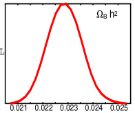
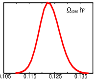
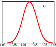
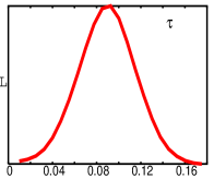
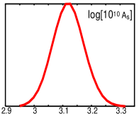
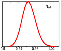
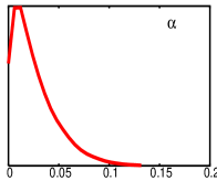
Figure 1: The one dimensional distributions of the sampled parameters.

The one dimensional posterior probability distributions for sampled and derived parameters are depicted in Fig. 1. In particular, the bestfit value for $\alpha$ is $\alpha=8\times 10^{-4}$, and the $2\sigma$ bound for the marginalized distribution is:

$$\alpha<0.08~{}\textrm{at}~{}95\%~{}\rm{c.l}$$ (41)

while for $\omega_{\rm cdm}$ we get:

$$\omega_{\rm cdm}=0.123\pm 0.008~{}\textrm{at}~{}95\%~{}\rm{c.l}.$$ (42)

Finally, our results for the amplitude of the primordial curvature spectrum gives the relation

$$\epsilon_{k}\sim 3\times 10^{8}\left(\frac{M_{\rm inf}}{M_{\rm P}}\right)^{4}~{}.$$ (43)

Substituting in Eq. (40), we see that the bound $\alpha<0.08$ finally provides the constraint

$$M_{\rm inf}\leq 10^{13}{\rm GeV}\left(\frac{f_{a}}{10^{12}\,{\rm GeV}}\right)^{5/24}~{},$$ (44)

corresponding to the central (yellow-)shaded forbidden region in Figs. 2, 3. As explained in Section III, this bound does not apply when thermal fluctuations induce PQ symmetry restoration after reheating, and we also assume –as in the rest of the literature– that it does not hold when quantum de Sitter fluctuations induce PQ symmetry restoration during inflation (although we believe that this issue is not completely clear and deserves further study). So, for sufficiently large $H_{\rm inf}$ and/or $\epsilon_{\rm eff}$, the isocurvature constraint does not apply above a given line in the $(M_{\rm inf},\,f_{a})$ plane, and the allowed region is split in two parts (as in Fig. 3).

V Discussion

V.1 General case

The constraints discussed in the last section –and in particular the isocurvature mode limit– exclude a large region in parameter space, and preserve only two regions. The first one depends on the reheating efficiency,

$$10^{10}\,{\rm GeV}<f_{a}<1.2\times 10^{11}\,{\rm GeV}\,,$$

$$5\times 10^{14}F(\epsilon_{\rm eff},f_{a})\,{\rm GeV}<M_{\rm inf}<3\times 10^{16}\,{\rm GeV}\,,$$ (45)

with

$$F(\epsilon_{\rm eff},f_{a})\equiv\min\left\{\sqrt{\frac{f_{a}}{10^{10}\,{\rm GeV}}}\,\,,\,\,\sqrt{\frac{1.4\times 10^{-8}}{\epsilon_{\rm eff}}}\frac{f_{a}}{10^{10}\,{\rm GeV}}\right\}\,.$$ (46)

The second one, for which the isocurvature mode is too small to be excluded by current cosmological data, corresponds to

$$10^{10}\,{\rm GeV}<f_{a}<2.5\times 10^{11}\,{\rm GeV}\,,\hskip 14.22636ptM_{\rm inf}<8\times 10^{12}\,{\rm GeV}\,,$$ (47)

where we assumed that the average misalignment angle in the observable universe is of order one: otherwise, the upper bound on $f_{a}$ could be relaxed significantly, while that on $M_{\rm inf}$ would only increase slightly, as $f_{a}$ to the power $5/24$, see Eq. (44).

For a large class of well-known inflationary models, $M_{\rm inf}$ is typically of the order of $10^{15}$ or $10^{16}$ GeV, and the relevant allowed window (if any) is the first one. In the next section, we feature the example of chaotic inflation with a quadratic potential. However, the second window (47) is also relevant, since it is possible to build low-scale inflationary model compatible with WMAP constraints and satisfying $M_{\rm inf}<8\times 10^{12}$ GeV. Actually, the main motivation for the original hybrid inflation model of Ref. hybrid was precisely the possibility to evade axionic isocurvature constraints. Nowadays, many low scale inflation models can be built in the generic framework of hybrid inflation (see Ref. LythRiotto for a review, or Allahverdi:2006iq for a recent example). In this case, the isocurvature perturbations carried by the axion are too small to be constrained by current data, and under the conditions of (47) the PQ axion model is perfectly viable.

V.2 Bounds for chaotic inflation with a quadratic potential

Inflation with a monomial potential $V(\phi)\propto\phi^{\alpha}$ is usually called chaotic inflation. The latest WMAP results combined with other data sets essentially rule out cases with $\alpha>4$, while the quartic case $\alpha=4$ is only in marginal agreement with the data. Therefore, in this section we only consider the case of a quadratic potential $V(\phi)=\frac{1}{2}m^{2}\phi^{2}$, still favored by observational bounds.

Using the COBE normalization, it is possible to prove that the mass should be of order $m\sim 1.3\times 10^{-6}\,M_{\rm P}$, and to show that $N_{e}$ e-folds before the end of inflation,

$$\phi_{e}^{2}=\frac{N_{e}}{2\pi}M_{\rm P}^{2}~{}.$$ (48)

In particular, between $N_{\rm obs}$ and $N_{\rm QCD}$, the scale of inflation should be in the range

$$1.5\times 10^{16}\,{\rm GeV}< M_{\rm inf} <2\times 10^{16}\,{\rm GeV}\,,$$

$$8\times 10^{13}\,{\rm GeV}< H_{\rm inf} <1\times 10^{14}\,{\rm GeV}\,.$$ (49)

So, if $f_{a}$ is close to $10^{10}$ or $10^{11}$ GeV, one has $H_{\rm inf}/2\pi\geq f_{a}$ and the PQ symmetry is broken by quantum fluctuations during inflation. If these fluctuations erase the isocurvature modes on cosmological scales as suggested by Ref. LythStewart2 , then chaotic inflation is compatible with the axion scenario.

We could hope to find a second allowed window in the case where $f_{a}$ is very large and the misalignment angle is fine-tuned to a very small value (i.e., inside the light green region in Figs. 2, 3). Note that this is not possible, at least in the case of chaotic inflation. Indeed, reheating after chaotic inflation is expected to lead to a temperature $T_{\rm rh}$ of the order of $10^{10}$ or $10^{11}$ GeV. So, if $f_{a}$ is much bigger than $10^{11}$GeV, thermal symmetry restoration after inflation cannot take place, and isocurvature bounds are applicable. Given the value of $M_{\rm inf}$ in Eq. (V.2), the isocurvature constraint (44) would enforce $f_{a}\geq 7\times 10^{27}\,{\rm GeV}\gg M_{\rm P}$, which is not realistic.

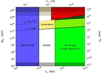
Figure 2: Bounds in the $(M_{\rm inf},\,f_{a})$ plane, assuming that reheating is very inefficient and the PQ symmetry can never be thermally restored ($\epsilon_{\rm eff}\leq 4\times 10^{-12}$). The energy scale of inflation $M_{\rm inf}$ is bounded from above by $r<0.3$ (top hatched) and from below by the requirement of successful baryogenesis (bottom hatched). Possible values of the PQ scale $f_{a}$ lie between the regions excluded by supernovae (left blue) and by the bound on the axionic relic density, produced by one of the following two mechanisms: axionic string decay (red) or misalignment angle at the time of the QCD transition (green). For the bounds related to the relic density, we use a solid line for the model independent bound (with a minimal, fine-tuned value of the misalignment angle), and a dotted line for the model dependent bound (with a generic misalignment angle of order one). The yellow region is excluded by the limit on the isocurvature mode amplitude $\alpha$: this is the main result of this work. If large quantum fluctuations during inflation can erase isocurvature modes on cosmological scale (as suggested by Ref. LythStewart2 ), the isocurvature bound does not apply above the line corresponding to $f_{a}=H_{\rm inf}/2\pi$. The remaining allowed regions are left in white. Details are explained in the text.

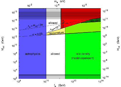
Figure 3: Same as previous figure, but assuming now that reheating is very efficient ($\epsilon_{\rm eff}=10^{-4}$) so that the the PQ symmetry is thermally restored above the dotted line. In this case, the constraint from string production and decay (red) extends to smaller values of $M_{\rm inf}$, but above the dotted line and for $10^{10}{\rm GeV}<f_{a}<1.2\times 10^{11}{\rm GeV}$ there is a new allowed region (corresponding to the erasure of isocurvature perturbations in the thermal bath).

V.3 Possible loopholes

In this subsection we will explore those loopholes we have left open for the axion to be the dominant component of cold dark matter.

V.3.1 Production of cosmic strings during reheating

Even if the reheating temperature of the universe is too low for a thermal phase transition at the Peccei-Quinn scale, it is possible that axionic cosmic strings be formed during preheating if the field responsible for symmetry breaking at the end of inflation is the Peccei-Quinn field. Then, the residual global $U(1)$ symmetry of the vacuum gives rise to axionic cosmic strings. At present there is no prediction for what is the scaling limit of such a mesh of strings produced during preheating. A crucial quantity that requires evaluation is the fraction of energy density in infinite strings produced at preheating, since they are the ones that will give the largest contribution to the axion energy density. It could then be that axionic strings produced at preheating may be responsible for the present axion abundance. We leave for the future the investigation of this interesting possibility.

V.3.2 Axion dilution by late inflation

When imposing bounds on the axion mass from its present abundance, it is assumed that no there is no significant late entropy production dilution or dilution from a secondary stage of inflation. We truly don’t know. It has been speculated that a short period of inflation may be required for electroweak baryogenesis to proceed Garcia-Bellido:1999 . In such a case, a few e-folds ($N\sim 5$) of late inflation may dilute the actual axion energy density by a factor $\gamma=e^{-3N}\sim 10^{-7}$, easily evading the bounds.

V.3.3 Coupling between radial part of PQ field and other fields.

The radial part of the PQ field could interact with other fields, including the inflaton (see e.g. hybrid ). Then the effective $f_{a}$ during inflation might be anything, and the isocurvature bounds might be alleviated.

VI Conclusions

In this paper, we reanalyzed the bounds on the cosmological scenario in which the cold dark matter is composed of axions plus some other component (like e.g. neutralinos), and the energy density of axions is produced by the misalignment mechanism at the time of the QCD transition. In this case, a fraction of the cosmological perturbations consists of isocurvature modes related to the quantum perturbations of the axion during inflation. We use this possible signature plus the contribution to dark matter energy density as a tracer of axions in the universe. In that sense, this work is similar to that presented in Sikivie:2006ir . However, we make a stronger statement about the generation of isocurvature modes in the case in which the PQ symmetry is restored by quantum fluctuations during inflation, and we significantly improve previous bounds coming from the non-observation of isocurvature modes in the CMB, in particular, given the recent WMAP 3-year data.

A narrow window for the PQ scale $10^{10}\,{\rm GeV}<f_{a}<10^{12}$ GeV still remains open, but we show that the main consequence of recent data on cosmological perturbations is to limit the possible energy scale of inflation in this context, in order not to have an excessively large contribution of isocurvature perturbations to the CMB anisotropies. In particular, we show that in the axion scenario, the energy scale of inflation cannot be in the range $8\times 10^{12}<M_{\inf}<5\times 10^{14}$ GeV, unless one of the two situations occurs: either reheating leads to a temperature $T_{\rm rh}>f_{a}$, with an efficiency parameter $\epsilon_{\rm eff}\geq 4\times 10^{-12}$, and there is another allowed region with $6\times 10^{10}\epsilon_{\rm eff}^{-1/2}\,{\rm GeV}<M_{\rm inf}<3\times 10^{16}$ GeV; or the misalignment angle is fine-tuned to very small values (this coincidence can be motivated by anthropic considerations) and the upper bound $M_{\inf}<10^{13}$ GeV can be slightly weakened (by at most one order of magnitude).

These bounds may be of interest taking into account particle physics experiments searching for the axion, which may help to put very stringent constraints on inflationary models. Detecting the QCD axion could shed some light on the scale of inflation and possibly into the mechanism responsible for inflation.

In this respect, there is an intriguing possibility that the PVLAS experiment PVLAS may have observed a pseudo-scalar particle coupled to photons. The nature of this particle is yet to be decided, since its properties seem in conflict with present bounds on the axion coupling to matter ADMX ; CAST , see however Masso ; Mendonca .

References

References

- (1) See e.g. the reviews: J.E. Kim, Phys. Rep. 150 (1987) 1; H.-Y. Cheng, Phys. Rep. 158 (1988) 1; R.D. Peccei, in ’CP Violation’, ed. by C. Jarlskog, World Scientific Publ., 1989, pp 503-551; M.S. Turner, Phys. Rep. 197 (1990) 67; G.G. Raffelt, Phys. Rep. 198 (1990) 1.
- (2) R. D. Peccei and H. Quinn, Phys. Rev. Lett. 38 (1977) 1440; Phys. Rev. D16 (1977) 1791.
- (3) S. Weinberg, Phys. Rev. Lett. 40 (1978) 223; F. Wilczek, Phys. Rev. Lett. 40 (1978) 279.
- (4) D. Harari and P. Sikivie, Phys. Lett. B195 (1987) 361; C. Hagmann and P. Sikivie, Nucl. Phys. B363 (1991) 247; C. Hagmann, S. Chang and P. Sikivie, Phys. Rev. D63 (2001) 125018.
- (5) D. H. Lyth and E. D. Stewart, Phys. Rev. D 46 (1992) 532; Phys. Lett. B283 (1992) 189.
- (6) C. Vafa and E. Witten, Phys. Rev. Lett. 53 (1984) 535.
- (7) D. J. Gross, R. D. Pisarski and L. G. Yaffe, Rev. Mod. Phys. 53 (1981) 43.
- (8) P. Fox, A. Pierce and S. D. Thomas, “Probing a QCD string axion with precision cosmological measurements,” arXiv:hep-th/0409059.
- (9) Particle Data Group, http://pdg.lbl.gov
- (10) S. Weinberg, Phys. Rev. Lett. 40 (1978) 223; W.A. Bardeen and S.-H.H. Tye, Phys. Lett. B74 (1978) 229; J. Ellis and M.K. Gaillard, Nucl. Phys. B150 (1979) 141; T.W. Donnelly et al., Phys. Rev. D18 (1978) 1607; D.B. Kaplan, Nucl. Phys. B260 (1985) 215; M. Srednicki, Nucl. Phys. B260 (1985) 689.
- (11) J. Kim, Phys. Rev. Lett. 43 (1979) 103; M. A. Shifman, A. I. Vainshtein and V. I. Zakharov, Nucl. Phys. B166 (1980) 493.
-
(12)
M. Dine, W. Fischler and M. Srednicki, Phys. Lett. B104 (1981)
199;
A. P. Zhitnitskii, Sov. J. Nucl. 31 (1980) 260. - (13) http://www.phys.ufl.edu/ axion/
- (14) http://cast.web.cern.ch/CAST/
-
(15)
K. Zioutas et al. [CAST Collaboration],
Phys. Rev. Lett. 94 (2005) 121301;
L. Duffy et al. [ADMX Collaboration], Phys. Rev. Lett. 95 (2005) 091304 - (16) M. Axenides, R. H. Brandenberger and M. S. Turner, Phys. Lett. B 126 (1983) 178.
- (17) A. D. Linde, JETP Lett. 40 (1984) 1333 [Pisma Zh. Eksp. Teor. Fiz. 40 (1984) 496]; Phys. Lett. B 158, 375 (1985); Phys. Lett. B 201 (1988) 437.
- (18) D. Seckel and M. S. Turner, Phys. Rev. D 32 (1985) 3178.
- (19) A. D. Linde, Phys. Lett. B 259 (1991) 38.
- (20) M. S. Turner and F. Wilczek, Phys. Rev. Lett. 66 (1991) 5.
- (21) A. D. Linde and D. H. Lyth, Phys. Lett. B 246 (1990) 353.
- (22) D. H. Lyth, Phys. Rev. D 45 (1992) 3394.
- (23) E. P. S. Shellard and R. A. Battye, arXiv:astro-ph/9802216.
- (24) E. W. Kolb and M. S. Turner,“The Early Universe”, Addison-Weseley (1990).
- (25) D. N. Spergel et al., “Wilkinson Microwave Anisotropy Probe (WMAP) three year results: Implications for cosmology,” arXiv:astro-ph/0603449.
- (26) S. Hannestad, A. Mirizzi and G. Raffelt, JCAP 0507 (2005) 002.
- (27) R.A. Battye and E.P.S. Shellard, Phys. Rev. Lett. 73 (1994) 2954; E.P.S. Shellard and R.A. Battye, Phys. Rept. 307 (1998) 227; R.A. Battye and E.P.S. Shellard, Nucl. Phys. Proc. Suppl. 72 (1999) 88
- (28) M. Yamaguchi, M. Kawasaki and J. Yokoyama, Phys. Rev. Lett. 82 (1999) 4578.
- (29) A. S. Sakharov and M. Y. Khlopov, Phys. Atom. Nucl. 57, 485 (1994) [Yad. Fiz. 57, 514 (1994)]; A. S. Sakharov, D. D. Sokoloff and M. Y. Khlopov, Phys. Atom. Nucl. 59, 1005 (1996) [Yad. Fiz. 59N6, 1050 (1996)]; M. Y. Khlopov, A. S. Sakharov and D. D. Sokoloff, arXiv:hep-ph/9812286; Nucl. Phys. Proc. Suppl. 72 (1999) 105.
- (30) P. Sikivie, Phys. Rev. Lett. 48 (1982) 1156.
- (31) S. Chang, C. Hagmann and P. Sikivie, Phys. Rev. D59 (1999) 023505.
- (32) M. S. Turner, Phys. Rev. D33 (1986) 889.
- (33) S. Weinberg, Phys. Rev. D 70, 083522 (2004).
- (34) D. Polarski and A. A. Starobinsky, Phys. Rev. D 50, 6123 (1994); M. Sasaki and E. D. Stewart, Prog. Theor. Phys. 95, 71 (1996); M. Sasaki and T. Tanaka, Prog. Theor. Phys. 99, 763 (1998).
- (35) J. García-Bellido and D. Wands, Phys. Rev. D 53, 5437 (1996); 52, 6739 (1995).
- (36) C. Gordon, D. Wands, B. A. Bassett and R. Maartens, Phys. Rev. D 63, 023506 (2001); N. Bartolo, S. Matarrese and A. Riotto, Phys. Rev. D 64, 123504 (2001). D. Wands, N. Bartolo, S. Matarrese and A. Riotto, Phys. Rev. D 66, 043520 (2002).
- (37) A. R. Liddle and D. H. Lyth, “Cosmological inflation and large-scale structure,” Cambridge University Press (2000).
- (38) P. Crotty, J. García-Bellido, J. Lesgourgues and A. Riazuelo, Phys. Rev. Lett. 91 (2003) 171301.
- (39) M. Beltrán, J. García-Bellido, J. Lesgourgues and A. Riazuelo, Phys. Rev. D 70, 103530 (2004).
- (40) M. Beltrán, J. García-Bellido, J. Lesgourgues, A. R. Liddle and A. Slosar, Phys. Rev. D 71 (2005) 063532.
- (41) M. Beltrán, J. García-Bellido, J. Lesgourgues and M. Viel, Phys. Rev. D 72 (2005) 103515.
- (42) A.D. Linde, “Particle Physics and Inflationary Cosmology”, Harwood Academic Press (1990).
- (43) M. Tegmark, A. Aguirre, M. Rees and F. Wilczek, Phys. Rev. D 73 (2006) 023505.
- (44) R. Rebolo et al. [VSA Collaboration], Mon. Not. Roy. Astron. Soc. 353, 747 (2004); C. Dickinson et al., Mon. Not. Roy. Astron. Soc. 353, 732 (2004).
- (45) T. J. Pearson et al. [CBI Collaboration], Astrophys. J. 591, 556 (2003); J. L. Sievers et al., Astrophys. J. 591, 599 (2003); A. C. S. Readhead et al., Astrophys. J. 609, 498 (2004).
- (46) C. l. Kuo et al. [ACBAR Collaboration], Astrophys. J. 600, 32 (2004); J. H. Goldstein et al., Astrophys. J. 599, 773 (2003).
- (47) J. A. Peacock et al. [2dFGRS Collaboration], Nature 410, 169 (2001); W. J. Percival et al., Mon. Not. R. Astron. Soc. A 327, 1297 (2001); 337, 1068 (2002).
- (48) M. Tegmark et al. [SDSS Collaboration], Astrophys. J. 606, 702 (2004).
- (49) S. Perlmutter et al. [Supernova Cosmology Project Collaboration], “Measurements of Omega and Lambda from 42 High-Redshift Supernovae,” Astrophys. J. 517 (1999) 565 [arXiv:astro-ph/9812133].
- (50) A. Lewis and S. Bridle, Phys. Rev. D 66, 103511 (2002); CosmoMC home page: http://www.cosmologist.info
- (51) S. Brooks and A. Gelman, JCGS, 7:434-456 (1998).
- (52) D. H. Lyth and A. Riotto, Phys. Rept. 314 (1999) 1.
- (53) R. Allahverdi, K. Enqvist, J. Garcia-Bellido and A. Mazumdar, Phys. Rev. Lett. 97 (2006) 191304
- (54) P. J. Steinhardt and M. S. Turner, Phys. Lett. B129 (1983) 51; G. Lazarides, R. Schaefer, D. Seckel and Q. Shafi, Nucl. Phys. B346 (1990) 193.
- (55) J. Garcia-Bellido, D. Y. Grigoriev, A. Kusenko and M. E. Shaposhnikov, Phys. Rev. D 60 (1999) 123504.
- (56) P. Sikivie, “The search for dark matter axions,” arXiv:hep-ph/0606014.
- (57) E. Zavattini et al. [PVLAS Collaboration], arXiv:hep-ex/0512022.
- (58) E. Masso and J. Redondo, JCAP 0509 (2005) 015.
- (59) J. T. Mendonca, J. Dias de Deus and P. Castelo Ferreira, Phys. Rev. Lett. 97 (2006) 100403.