Two modes of searching for new neutrino interactions at MINOS

Abstract

The SuperKamiokande atmospheric neutrino measurements leave substantial room for nonstandard interactions (NSI) of neutrinos with matter in the $\nu_{e}-\nu_{\tau}$ sector. Large values of the NSI couplings are accommodated if the vacuum oscillation parameters are changed from their standard values. Short and medium baseline neutrino beams can break this degeneracy by measuring the true vacuum oscillation parameters with the $\mathrel{{\nu_{\mu}}}$ disappearance mode, for which the matter effects are negligible or subdominant. These experiments can also search for the $\nu_{e}-\nu_{\tau}$ flavor changing effects directly, by looking for $\mathrel{{\nu_{\mu}}}-\mathrel{{\nu_{e}}}$ conversion caused by the intervening matter. We discuss both of these methods for the case of MINOS. We find that, while the present MINOS data on $\mathrel{{\nu_{\mu}}}$ disappearance induce only minor changes on the constraints on the NSI parameters, the situation will improve markedly with the planned increase of the statistics by an order of magnitude. In that case, the precision will be enough to distinguish certain presently allowed NSI scenarios from the no-NSI case. NSI per quark of about 10% the size of the standard weak interaction could give a $\mathrel{{\nu_{\mu}}}-\mathrel{{\nu_{e}}}$ conversion probability of the order $\sim 10^{-2}$, measurable by MINOS in the same high statistics scenario. In this $\mathrel{{\nu_{\mu}}}-\mathrel{{\nu_{e}}}$ channel, the small effects of NSI could be comparable or larger than the vacuum contribution of the small angle $\theta_{13}$. The expected $\theta_{13}$ bound at MINOS should be more properly interpreted as a bound in the $\theta_{13}$ – NSI parameter space.

I Introduction

Neutrinos offer certain unique advantages for the search of new forces beyond the Standard Model. These advantages stem from the fact that neutrinos are sensitive only to the weakest known forces, the weak interaction and gravity, and therefore offer a “cleaner” ground – with respect to other particles – to look for the subdominant effects of the new, nonstandard interactions (NSI). The abundance of neutrinos from natural sources (chiefly the Sun and the interaction of cosmic rays in the Earth’s atmosphere) adds further motivation.

The very same reason that makes them an interesting probe, the weakness of their interactions, also made the neutrinos historically difficult to study experimentally. The result is that to this day some of the neutrino interactions are very poorly known, with uncertainties comparable to, or even exceeding, the standard model predictions. In the case of neutrino-matter interactions the measurements of neutrino cross sections at CHARM and NuTeV Vilain et al. (1994); Zeller et al. (2002) constrain chiefly the coupling of the muon neutrino, while leaving the $\mathrel{{\nu_{e}}}-\mathrel{{\nu_{\tau}}}$ channels largely unconstrained (see Berezhiani and Rossi (2002); Davidson et al. (2003) for a comprehensive discussion).

Measurements of neutrino matter effects at neutrino oscillation experiments offer increased sensitivity to neutral current NSI in the $e-\tau$ sector, down to tens of per cent of the weak interaction strength Fornengo et al. (2002); Guzzo et al. (2002); Gonzalez-Garcia and Maltoni (2004). Still, however, certain directions in the parameter space exist where large NSI are allowed, because their effect on the oscillations of solar and atmospheric neutrinos is degenerate with that of the mixings and mass square differences Friedland et al. (2004a, b); Friedland and Lunardini (2005).

Logically, the next step towards stronger constraints – or discovery – of neutrino NSI is to break these degeneracies. One way to do so is to perform precision measurements of the neutrino mixings and mass squared differences in conditions where matter effects are negligible or subdominant. Such conditions of “quasi-vacuum” are realized in the $\mathrel{{\nu_{\mu}}}-\mathrel{{\nu_{\tau}}}$ oscillation channel of the $\mathrel{{\nu_{\mu}}}$ beams used by K2K Ahn et al. (2003); Aliu et al. (2005) and MINOS Adamson et al. (2006); Petyt (2006). There, the large $\mathrel{{\nu_{\mu}}}-\mathrel{{\nu_{\tau}}}$ (vacuum) mixing, $\theta_{23}$, induces oscillations effects of order unity. These dominate over the matter effects, which are at most of order $\sim 10^{-1}$, due to the small matter width along the beam trajectory.

In a recent paper Friedland and Lunardini (2005) we showed how the data from K2K, in combination with the SuperKamiokande atmospheric neutrino measurements, restrict the allowed region of the NSI couplings. The conclusion was that, while improving with respect to the atmospheric data only, the combined data still allow couplings of order unity (relative to the Fermi constant, $G_{F}$).

Here we discuss how the situation changes in light of the recently reported search for $\mathrel{{\nu_{\mu}}}$ disappearance at MINOS Petyt (2006). We also illustrate the increased potential that MINOS will have with higher statistics. We get that with the present MINOS data the presence of NSI is neither revealed nor excluded. The allowed region of the NSI parameters is changed only slightly. Qualitative improvements are expected, however, with the planned increase of statistics by an order of magnitude. The precision in that case would be such that in certain NSI scenarios (with the NSI couplings on both $u$ and $d$ quarks of the order of 10% of the weak interaction), the point of zero NSI would be allowed only with confidence level higher than 99%.

A second way to search for the flavor-changing $\mathrel{{\nu_{e}}}-\mathrel{{\nu_{\tau}}}$ NSI is to look for the $\mathrel{{\nu_{\mu}}}-\mathrel{{\nu_{e}}}$ conversion Gago et al. (2001); Huber et al. (2002a); Campanelli and Romanino (2002); Blennow et al. (2005); Huber et al. (2002b). In this channel, the vacuum contribution to the oscillations of beam neutrinos is due to the small mixing angle $\theta_{13}$. Considering that $\sin^{2}2\theta_{13}\mathrel{\vbox{\hbox{$<$}\nointerlineskip\hbox{$\sim$}}}0.14$ Apollonio et al. (1999, 2003) we see that at K2K and MINOS the NSI effects could be of the same order or larger than the vacuum ones, and therefore they could be visible in spite of their smallness on absolute scale. In this paper we illustrate this point for the specific case of MINOS, and show that a conversion probability of $\sim 0.05$, within the reach of MINOS, could be due to NSI within the currently allowed region, with couplings per quark of the order of 10% of the weak interaction.

Finally, although not discussed here, another important method of searching for new tau neutrino interactions at MINOS is by measuring the neutral current event rate in the far detector, where a large fraction of events should be due to tau neutrinos generated by oscillations. The combinations of the NSI parameters probed in this method do not uniquely map to those probed by the matter effects studied here Friedland and Lunardini (2005), hence providing a complementary probe of NSI.

In Sec. II we describe the parametrization of the nonstandard interactions being probed, list various constraints on these interactions and give the resulting oscillation Hamiltonian. We also review the main results of our earlier study of NSI effects on atmospheric neutrinos (in Sect. II.2). In Sect. III we study the combined NSI sensitivity of the $\mathrel{{\nu_{\mu}}}\rightarrow\mathrel{{\nu_{\tau}}}$ mode at MINOS and atmospheric and K2K data. Sec. IV is devoted to the $\mathrel{{\nu_{\mu}}}\rightarrow\mathrel{{\nu_{e}}}$ appearance channel at MINOS. Finally, Sec. V summarizes our findings.

II Neutrino oscillations and NSI in the $\mathrel{{\nu_{e}}}-\mathrel{{\nu_{\tau}}}$ sector

II.1 Effective Lagrangian, bounds, oscillation Hamiltonian

The neutrino oscillation Hamiltonian in vacuum is dominated by the atmospheric mass splitting. In the flavor basis $\mathrel{{\nu_{e}}},\mathrel{{\nu_{\mu}}},\mathrel{{\nu_{\tau}}}$, this Hamiltonian is given by

$$H_{\rm vac}\simeq\Delta\left(\begin{array}[]{ccc}-1&0&0\\ 0&-\cos 2\theta&\sin 2\theta\\ 0&\sin 2\theta&\cos 2\theta\\ \end{array}\right),$$ (1)

where $\Delta\equiv\Delta m^{2}/(4E_{\nu})$, $E_{\nu}$ is the neutrino energy and $\Delta m^{2}$ is the largest mass square difference in the neutrino spectrum (often called $\Delta m^{2}_{32}$). Corrections to $H_{vac}$ due to the smaller, “solar” mass splitting and the remaining two mixing angles produce only subdominant effects on the $\mathrel{{\nu_{\mu}}}\rightarrow\mathrel{{\nu_{\tau}}}$ oscillations (see sec. III) and so will be omitted for the moment. See, e.g., Friedland and Lunardini (2005) for the full Hamiltonian including all these terms.

In matter, the neutrino propagation is affected by refraction (coherent forward scattering). We parameterize the corresponding part of the Hamiltonian as:

$$H_{\rm mat}=\sqrt{2}G_{F}n_{e}\begin{pmatrix}1+\mathrel{{\epsilon_{ee}}}&\epsilon_{e\mu}^{\ast}&\epsilon_{e\tau}^{\ast}\\ \mathrel{{\epsilon_{e\mu}}}&\mathrel{{\epsilon_{\mu\mu}}}&\epsilon_{\mu\tau}^{\ast}\\ \mathrel{{\epsilon_{e\tau}}}&\mathrel{{\epsilon_{\mu\tau}}}&\mathrel{{\epsilon_{\tau\tau}}}\\ \end{pmatrix}~{}$$ (2)

(up to an irrelevant constant). Here $n_{e}$ is the number density of electrons in the medium and the epsilon terms represent the contribution of the NSI.

The physical origin of the NSI terms in Eq. (2) can be the exchange of a new heavy vector or scalar particle, described by the effective low-energy four-fermion Lagrangian

$$L^{NSI} = -2\sqrt{2}G_{F}(\bar{\nu}_{\alpha}\gamma_{\rho}\nu_{\beta})(\epsilon_{\alpha\beta}^{f\tilde{f}L}\bar{f}_{L}\gamma^{\rho}\tilde{f}_{L}+\epsilon_{\alpha\beta}^{f\tilde{f}R}\bar{f}_{R}\gamma^{\rho}\tilde{f}_{R})$$ (3)

$$+ h.c.$$

Here $\epsilon_{\alpha\beta}^{f\tilde{f}L}$ ($\epsilon_{\alpha\beta}^{f\tilde{f}R}$) denotes the strength of the NSI between the neutrinos $\nu$ of flavors $\alpha$ and $\beta$ and the left-handed (right-handed) components of the fermions $f$ and $\tilde{f}$. The epsilons in Eq. (2) are the sum of the contributions from electrons ($\epsilon^{e}$), up quarks ($\epsilon^{u}$), and down quarks ($\epsilon^{d}$) in matter: $\epsilon_{\alpha\beta}\equiv\sum_{f=u,d,e}\epsilon_{\alpha\beta}^{f}n_{f}/n_{e}$. They are thus normalized per electron. In turn, $\epsilon_{\alpha\beta}^{f}\equiv\epsilon_{\alpha\beta}^{fL}+\epsilon_{\alpha\beta}^{fR}$ and $\epsilon_{\alpha\beta}^{fP}\equiv\epsilon_{\alpha\beta}^{ffP}$. Notice that the matter effects are sensitive only to the interactions that preserve the flavor of the background fermion $f$ (required by coherence Friedland and Lunardini (2003)) and, furthermore, only to the vector part of that interaction.

Neutrino scattering tests, like those of NuTeV Zeller et al. (2002) and CHARM Vilain et al. (1994), mainly constrain the NSI couplings of the muon neutrino, e.g., $|\mathrel{{\epsilon_{e\mu}}}|\lesssim 10^{-3}$, $|\mathrel{{\epsilon_{\mu\mu}}}|\lesssim 10^{-3}-10^{-2}$. The limits they place on $\mathrel{{\epsilon_{ee}}}$, $\mathrel{{\epsilon_{e\tau}}}$, and $\mathrel{{\epsilon_{\tau\tau}}}$ are rather loose, e. g., $|\epsilon_{\tau\tau}^{uuR}|<3$, $-0.4<\epsilon_{ee}^{uuR}<0.7$, $|\epsilon_{\tau e}^{uu}|<0.5$, $|\epsilon_{\tau e}^{dd}|<0.5$ Davidson et al. (2003). Stronger constraints exist on the corresponding interactions involving the charged leptons. Those, however, are model-dependent and do not apply if the NSI come from the underlying operators containing the Higgs fields Berezhiani and Rossi (2002). Here we are interested only in direct bounds that follow from experiments.

Given the above bounds we will set $\mathrel{{\epsilon_{e\mu}}}$ and $\mathrel{{\epsilon_{\mu\mu}}}$ to zero in our analysis. Furthermore, for simplicity we will also set $\mathrel{{\epsilon_{\mu\tau}}}$ to zero. The earlier analyses of the atmospheric neutrino data Fornengo et al. (2002) have indicated that this parameter is quite constrained ($\mathrel{{\epsilon_{\mu\tau}}}<10^{-2}-10^{-1}$). Here, as in our previous works, we have a three-dimensional NSI parameter space, spanned by $\mathrel{{\epsilon_{ee}}}$, $\mathrel{{\epsilon_{e\tau}}}$, and $\mathrel{{\epsilon_{\tau\tau}}}$.

II.2 Atmospheric neutrinos and NSI

The atmospheric neutrino flux is comprised of both neutrinos and antineutrinos, initially produced in the electron and muon flavor states, with the energy spectrum spanning roughly five orders of magnitude, from $10^{-1}$ to $10^{4}$ GeV Engel et al. (2000). The data can be divided into a high energy sample, $E_{\nu}\gtrsim 10$ GeV, where only the muon neutrino flux is measured (through-going and stopping muons sample), and a lower energy one, where both the muon and electron neutrino data are available. For the first, the data show disappearance of $\mathrel{{\nu_{\mu}}}$ with large suppression at lower energies/longer baselines and smaller suppression in the opposite limits; the second sample is consistent with no oscillations of $\mathrel{{\nu_{e}}}$ and $\mathrel{{\nu_{\mu}}}$ disappearance with large amplitude. This means that the $\mathrel{{\nu_{\mu}}}$ oscillate into $\mathrel{{\nu_{\tau}}}$ at low energy, and that the $\mathrel{{\nu_{\mu}}}$ data are well described by vacuum oscillations with large mixing at all energies.

One way to fit these data is to require that the NSI couplings of the tau neutrino are negligible at all energies. For example, if $\mathrel{{\epsilon_{e\tau}}}=0$, we would need $\sqrt{2}\mathrel{{\epsilon_{\tau\tau}}}G_{F}n_{e}\mathrel{\vbox{\hbox{$<$}\nointerlineskip\hbox{$\sim$}}}\Delta m^{2}/(2E_{0})$ at $E_{0}\sim 20-30$ GeV (the highest energy where an oscillation maximum occurs for neutrinos traveling along the diameter of the Earth), to ensure that $\mathrel{{\nu_{\mu}}}$ oscillates into $\mathrel{{\nu_{\tau}}}$ with unsuppressed amplitude in the high energy data sample. Substituting numerical values, this translates into the bound $|\mathrel{{\epsilon_{\tau\tau}}}|\lesssim 0.2$ Friedland et al. (2004b).

In Friedland et al. (2004b) we pointed out another possibility: one of the two (non-zero) eigenvalues of $H_{mat}$ is small with respect to the vacuum terms, so that at high energy $\mathrel{{\nu_{\mu}}}$ can oscillate into the corresponding eigenstate, $\mathrel{{\nu_{\tau}}}^{\prime}$, without suppression. Specializing to the case which is continuously connected to the standard $\mathrel{{\nu_{\mu}}}-\mathrel{{\nu_{\tau}}}$ oscillation scenario (i.e., $\mathrel{{\nu_{\tau}}}^{\prime}$ becomes $\mathrel{{\nu_{\tau}}}$ in the limit of no NSI), this gives:

$$|1+\mathrel{{\epsilon_{ee}}}+\mathrel{{\epsilon_{\tau\tau}}}-\sqrt{(1+\mathrel{{\epsilon_{ee}}}-\mathrel{{\epsilon_{\tau\tau}}})^{2}+4|\mathrel{{\epsilon_{e\tau}}}|^{2}}|\lesssim 0.4~{}.$$ (4)

Although at high energy $\mathrel{{\nu_{\mu}}}$’s oscillate into a mixture of $\mathrel{{\nu_{\tau}}}$ and $\mathrel{{\nu_{e}}}$, and not purely into $\mathrel{{\nu_{\tau}}}$, this is not observable, given the absence of $\mathrel{{\nu_{e}}}$ data in the high energy sample. At lower energy, where the kinetic terms of the Hamiltonian dominate, the $\mathrel{{\nu_{e}}}$ flux is unoscillated, as the muon neutrinos oscillate dominantly into $\mathrel{{\nu_{\tau}}}$.

The condition (4) describes the allowed region of the epsilons; it has the shape of a parabola centered on the curve

$$\mathrel{{\epsilon_{\tau\tau}}}=|\mathrel{{\epsilon_{e\tau}}}|^{2}/(1+\mathrel{{\epsilon_{ee}}})~{}.$$ (5)

It is also independent of the phase/sign of $\mathrel{{\epsilon_{e\tau}}}$.

The conversion of $\mathrel{{\nu_{\mu}}}$ at high energy mimics vacuum oscillations with an effective mass splitting, $\Delta m^{2}_{m}$, and an effective mixing angle, $\theta_{m}$, given by Friedland et al. (2004b); Friedland and Lunardini (2005):

$$\Delta m^{2}_{m}=\Delta m^{2}\left[(c_{2\theta}(1+c^{2}_{\beta})-s^{2}_{\beta})^{2}/4+(s_{2\theta}c_{\beta})^{2}\right]^{1/2}~{},$$

$$\tan 2\theta_{m}=2s_{2\theta}c_{\beta}/(c_{2\theta}(1+c^{2}_{\beta})-s^{2}_{\beta})~{}.$$ (6)

They depend on the NSI only through the angle $\beta$, defined as

$$\tan 2\beta=2|\mathrel{{\epsilon_{e\tau}}}|/(1+\mathrel{{\epsilon_{ee}}}-\mathrel{{\epsilon_{\tau\tau}}})~{}.$$ (7)

If NSI are present but ignored in the data analysis, the highest energy neutrino data would give $\theta_{m}$ and $\Delta m^{2}_{m}$ instead of the vacuum parameters. Those can be inferred from Eq. (6). Taking the experimentally favored value $\theta_{m}=\pi/4$, we find:

$$\Delta m^{2}\simeq\Delta m^{2}_{m}(1+\cos^{-2}\beta)/2~{},\hskip 14.22636pt\sin^{2}\theta=\frac{\Delta m^{2}_{m}}{2\Delta m^{2}}~{}.$$ (8)

We see that the vacuum mass splitting is larger than the measured one, $\Delta m^{2}_{m}$, and the vacuum mixing $\theta$ is smaller than maximal ($\theta<\pi/4$).

The vacuum parameters are constrained by data from lower energy atmospheric neutrinos, $E\mathrel{\vbox{\hbox{$<$}\nointerlineskip\hbox{$\sim$}}}1$ GeV, for which the vacuum term of the Hamiltonian dominates. Calling $\theta_{min}$ and $\Delta m^{2}_{max}$ the smallest mixing and the largest mass splitting allowed by those, we have two constraints on $\beta$ Friedland and Lunardini (2005):

$$\cos^{2}\beta\mathrel{\vbox{\hbox{$>$}\nointerlineskip\hbox{$\sim$}}}\tan^{2}\theta_{min}~{},\hskip 14.22636pt\cos^{2}\beta\geq\left[\frac{2\Delta m^{2}_{max}}{\Delta m^{2}_{m}}-1\right]^{-1}~{},$$ (9)

that follow from Eq. (8). These conditions truncate the allowed region (4), as shown in Friedland et al. (2004b); Friedland and Lunardini (2005).

Let us emphasize that the analytics in Eqs. (6)-(9) is for guidance only, since it relies on the over-restrictive condition (5) and on the approximation of negligible vacuum terms at $E\mathrel{\vbox{\hbox{$>$}\nointerlineskip\hbox{$\sim$}}}10$ GeV. The corrections due to the vacuum terms to the conditions (4) and (9) introduce a dependence on the mass hierarchy, i.e. on the sign of $\mathrel{{\Delta m^{2}}}$, with the inverted hierarchy ($\mathrel{{\Delta m^{2}}}<0$) giving a larger allowed region of the NSI. We refer to ref. Friedland and Lunardini (2005) for details on this and on the corrections due to the mixing angle $\theta_{13}$, which break the symmetry in the phase of $\mathrel{{\epsilon_{e\tau}}}$.

III $\mathrel{{\nu_{\mu}}}-\mathrel{{\nu_{\tau}}}$ oscillations at MINOS

III.1 General considerations for K2K and MINOS

For the setups of K2K and MINOS the neutrino oscillations in the $\mathrel{{\nu_{\mu}}}-\mathrel{{\nu_{\tau}}}$ channel are dominated by the vacuum contribution, with the matter effects playing only a subdominant role. This is proven by the fact that both beams have baselines much shorter than the characteristic length (or equivalently, the width, see Lunardini and Smirnov (2000)) which describes refraction effects, $l_{ref}=(\sqrt{2}G_{F}n_{e})^{-1}\simeq 1.9\cdot 10^{3}$ Km for the average density of the continental crust, $\rho=2.7~{}{\rm g\cdot cm^{-3}}$. Specifically, the K2K baseline is 250 Km long, only about a tenth of the refraction length, and this ensures that matter effects at K2K are negligible. MINOS, with its 735 Km long baseline, covers about 40% of $l_{ref}$, and therefore is expected to see matter effects at a subdominant, while not entirely negligible, level. For simplicity here we consider the zeroth order description of both K2K and MINOS in terms of vacuum oscillations only (and comment on the small corrections due to refraction effects at MINOS later, see sec. III.3).

In this approximation MINOS and K2K measure the oscillation parameters in vacuum, $\theta$ and $\Delta m^{2}$. The difference between $\theta,\Delta m^{2}$ and the corresponding parameters inferred from the atmospheric neutrino data tells us how much room there is for NSI, through Eqs. (8)-(9).

The present MINOS data (a similar description holds for K2K) can be fit by a range of $\Delta m^{2}$ and $\theta$, such that larger values of $\Delta m^{2}$ come with smaller values of $\theta$. Compared to the corresponding region from the SuperKamiokande atmospheric analysis, the MINOS region is relatively narrow in $\Delta m^{2}$, $\Delta m^{2}=(2.5-3.65)\mathrel{{\cdot 10^{-3}~{}{\rm eV^{2}}}}$ (at 68% confidence level, C.L.) Petyt (2006), but extended in $\theta$, with $\sin^{2}2\theta\simeq 0.73-1$ (68% C.L.). The MINOS constraint on $\Delta m^{2}$ also improves slightly on the analogous restriction given by K2K.

We notice that the region currently allowed by MINOS is extended in the direction (smaller $\theta$ comes with larger $\Delta m^{2}$) obtained from the NSI analysis of the atmospheric data. Due to this accidental degeneracy, we expect that the present-day MINOS results leave substantial room for the NSI, with only a loose upper bound on $\beta$ according to Eq. (9).

III.2 The data analysis: MINOS, SuperKamiokande, K2K

We have carried out a combined analysis of the atmospheric data from SuperKamiokande and $\nu_{\mu}\rightarrow\nu_{\tau}$ oscillation data from K2K and MINOS. Our study has two parts. First, we have investigated the impact of the recently released MINOS data on the existing NSI constraints. Second, to illustrate the expected future sensitivity of MINOS, we have simulated a future MINOS signal with projected higher statistics. For this simulation, we considered two scenarios: one which would give a signal of NSI, and another that would instead give a constraint on them.

The starting point in both cases are the results from our NSI analysis of the atmospheric neutrino data. This analysis was done in Friedland et al. (2004b) and Friedland and Lunardini (2005) and involved a fit to the complete 1489-day charged current Super-Kamiokande phase I data set Hayato (2004); Ashie et al. (2005), including the $e$-like and $\mu$-like data samples of sub- and multi-GeV contained events as well as the stopping and through-going upgoing muon data events. The details of the code, provided by Michele Maltoni, are given in Friedland et al. (2004b); Friedland and Lunardini (2005). In Friedland and Lunardini (2005) we have scanned a five-dimensional parameter space $(\mathrel{{\epsilon_{ee}}},\mathrel{{\epsilon_{e\tau}}},\mathrel{{\epsilon_{\tau\tau}}},\Delta m_{23}^{2},\sin^{2}\theta_{23})$ and obtained an allowed region in this space. The output of that scan – a set of $\chi^{2}$ values on a five-dimensional grid – was used here.

The output was combined with a $\chi^{2}$ array from the K2K vacuum oscillation analysis. The latter was provided by the K2K collaboration in tabular form, and refers to the published analysis of Ref. Aliu et al. (2005) (Fig. 4 there). Since that analysis is practically independent of the matter interactions, the same $\chi^{2}$ array was added to each $(\Delta m_{23}^{2},\sin^{2}\theta_{23})$ plane. For details, see again Friedland and Lunardini (2005).

Finally, we have performed a similar fit to the released MINOS data. The data used were the number of observed events in each MINOS energy bin versus the corresponding predictions without oscillations as given in Petyt (2006). Our analysis follows the one in Petyt (2006) as closely as possible. The resulting allowed region and the best-fit point agree reasonably well with those in the MINOS analysis (Petyt (2006), slide 60). The output of this fit was then combined with those of the SuperKamiokande and K2K analyses, giving a five-dimensional allowed region in the space $(\mathrel{{\epsilon_{ee}}},\mathrel{{\epsilon_{e\tau}}},\mathrel{{\epsilon_{\tau\tau}}},\Delta m_{23}^{2},\sin^{2}\theta_{23})$. The combined results were then marginalized, either over the NSI or over the oscillation parameters.

For the second part, we have simulated the data with increased statistics that might be expected in the future at MINOS. We have used statistics corresponding to $25\times 10^{20}$ protons-on-target (p.o.t.), as quoted by the MINOS collaboration (see, e.g., Petyt (2006)), henceforth referred to as “MINOS-high” sample. We have also checked how our results change with changing the statistics to $16\times 10^{20}$ p.o.t.

We have simulated future data by taking the histogram of the expected number of events in each energy bin published by the MINOS collaboration, scaling it up to the appropriate statistics, applying oscillations to it according to the set of parameters chosen and finally simulating statistical fluctuations in the data using Poisson statistics. It is hoped that this simplified procedure still captures the relevant effects. The most accurate way would of course be to perform a full Monte-Carlo simulation of the detector, which could be done by the MINOS collaboration.

The simulated data were then used as an input to the combined SuperKamiokande-K2K-MINOS analysis described before.

III.3 Results with present MINOS data

The results of our analysis of the existing data are presented in Figs. 1-2 and Table 1.

Fig. 1 shows the effect of adding the MINOS results on the allowed region in the space of $\sin^{2}\theta-\Delta m^{2}$. The contours show the case of the standard interactions, while the filled regions were found after marginalizing over the NSI (see the caption for details). The Figure also shows the direction in Eq. (8), along which $\sin^{2}\theta$ and $\Delta m^{2}$ would be found for fixed $\sin^{2}\theta_{m}$ and $\Delta m^{2}_{m}$ ($\Delta m^{2}_{m}=2.1\cdot 10^{-3}~{}{\rm eV^{2}}$ and $\theta_{m}=\pi/4$, motivated by the best fit to the atmospheric data only Ashie et al. (2005)) and NSI varying along the parabola (5).

For the case of no NSI we see that both with and without MINOS the best fit point lies at maximal mixing, with the interval $\sin^{2}\theta\simeq 0.3-0.7$ allowed at $3\sigma$ confidence level. These bounds on the mixing are due to the atmospheric data; the main effect of adding the MINOS data is to further restrict $\Delta m^{2}$: $\Delta m^{2}=(1.8-3.4)\mathrel{{\cdot 10^{-3}~{}{\rm eV^{2}}}}$ at $3\sigma$ C.L.

Both with and without MINOS, in the case with NSI the allowed region extends along the direction in Eq. (8), allowing smaller mixing and larger $\Delta m^{2}$ with respect to the standard case. Besides the restriction on $\Delta m^{2}$ already observed, adding the MINOS data has the effect to move the best fit point away from maximal mixing. The new best fit point has $\sin^{2}\theta=0.36$ and $\mathrel{{\Delta m^{2}}}=2.88\mathrel{{\cdot 10^{-3}~{}{\rm eV^{2}}}}$, and it lies along the curve (8) as it is plotted in the figure. This happens because the MINOS-only best fit point – $\sin^{2}\theta=0.33$ and $\mathrel{{\Delta m^{2}}}=3.05\mathrel{{\cdot 10^{-3}~{}{\rm eV^{2}}}}$ Petyt (2006) – lies near this curve and the atmospheric $\chi^{2}$ is very flat along this direction, once the NSI are included. It has to be stressed, however, that there is only an insignificant difference between the best fit point and, say, the minimum of $\chi^{2}$ along the direction $\theta=\pi/4$. The latter point is within the $68\%$ C.L. contour.

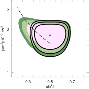
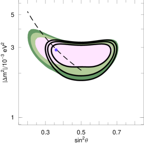
Figure 1: Regions in the space $\mathrel{{\Delta m^{2}}}-\sin^{2}\theta$ allowed by the global fit before (upper panel) and after (lower panel) the MINOS results, with purely standard interactions (contours) and with NSI (filled areas). For both cases we plot the regions allowed at 95%, 99% and $3\sigma$ confidence levels for 2 degrees of freedom. We have marginalized also over the sign of $\Delta m^{2}$ and took $-1\leq\mathrel{{\epsilon_{ee}}}\leq 1.6$, motivated by one of the accelerator bounds (see Friedland et al. (2004b)). The dashed line represents the possible positions of the best fit point of the atmospheric data only in the space of the vacuum parameters for fixed $\theta_{m}$ and $\Delta m^{2}_{m}$, and varying NSI along the parabola (5). We used $\Delta m^{2}_{m}=2.1\cdot 10^{-3}~{}{\rm eV^{2}}$ and $\theta_{m}=\pi/4$, motivated by the best fit of atmospheric neutrinos alone Ashie et al. (2005).

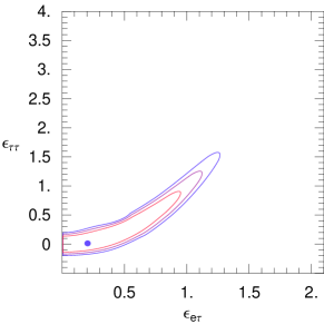
Figure 2: Two sections of the allowed region in the three dimensional space of the NSI couplings along the plane $\mathrel{{\epsilon_{ee}}}=0$. The contours refer to 95%, 99% and $3\sigma$ confidence levels. The points of minimum of the $\chi^{2}$ in this plane are also shown. The upper (lower) panel refers to normal (inverted) mass hierarchy. The $\mathrel{{\epsilon_{ee}}}<0$ regions are symmetric with respect to those shown.

The shift of the best fit point in the space of oscillation parameters indicates that with MINOS non-zero NSI are favored, even though in a statistically insignificant way. To check this, we have marginalized the likelihood over the oscillation parameters (with fixed mass hierarchy) to obtain the $\chi^{2}$ in the three dimensional space of the epsilons, $\chi^{2}(\mathrel{{\epsilon_{ee}}},\mathrel{{\epsilon_{\tau\tau}}},\mathrel{{\epsilon_{e\tau}}})$. We find that for the inverted mass hierarchy the minimum of this marginalized $\chi^{2}$ is at the point $(\mathrel{{\epsilon_{ee}}},\mathrel{{\epsilon_{\tau\tau}}},\mathrel{{\epsilon_{e\tau}}})=(0.6,0.933,0.615)$. This point is practically degenerate with others that satisfy the condition (5) and correspond to vacuum oscillation parameters (Eq. (8)) close to the MINOS-only best fit point. Again, we find that the difference in $\chi^{2}$ between the best fit point and the point with zero NSI is minimal and has no statistical significance.

In Fig. 1 the effects of matter on the MINOS signal were not taken into account for simplicity. We have checked that their inclusion leaves the results unchanged qualitatively, with only a change of the order of 10% in the extent of the upper left part of the allowed region (for the NSI case, shaded areas).

Fig. 2 shows sections of the 3D allowed region along the plane $\mathrel{{\epsilon_{ee}}}=0$ for normal and inverted mass hierarchy. The contours correspond to intervals of $\chi^{2}$ with respect to the absolute minimum given above and represent the regions allowed at 95%, 99% and $3\sigma$ confidence levels. They show only minor changes with respect to the same contours without MINOS Friedland and Lunardini (2005). For illustration in Fig. 2 we show the points of minimum of $\chi^{2}$ along the plane $\mathrel{{\epsilon_{ee}}}=0$. Those appear to be away from the origin, confirming what has been discussed about the shift of the best fit to non-zero NSI.

$\mathrel{{\epsilon_{ee}}}$	$|\mathrel{{\epsilon_{e\tau}}}|$ (99% C.L.)	$\mathrel{{\epsilon_{\tau\tau}}}$ (99% C.L.)	$\mathrel{{\epsilon_{e\tau}}},\mathrel{{\epsilon_{\tau\tau}}}$ (best)
-1	$<$0.3	$\left[-0.4,0.6\right]$	0, 0
-0.5	$<$0.75	$\left[-0.15,1.2\right]$	0.15, 0.1
0.	$<$1.65	$\left[-0.15,2.6\right]$	0.438, 0.255
0.3	$<$2.1	$\left[-0.15,3.4\right]$	0.67, 0.413
0.6	$<$2.5	$\left[-0.15,3.9\right]$	0.933, 0.615
0.9	$<$2.9	$\left[-0.15,4.5\right]$	1.019, 0.615

Table 1: Some relevant numbers describing the 3D allowed region of the NSI couplings for inverted mass hierarchy. We give the intervals of $\mathrel{{\epsilon_{e\tau}}}$ and of $\mathrel{{\epsilon_{\tau\tau}}}$ enclosed by the 99% C.L. region in planes of fixed $\mathrel{{\epsilon_{ee}}}$, and the values of $\mathrel{{\epsilon_{e\tau}}},\mathrel{{\epsilon_{\tau\tau}}}$ that minimize the $\chi^{2}$ in the same planes.

Table 1 gives further details on our results. It presents information on sections of the 3D allowed region along several planes of fixed $\mathrel{{\epsilon_{ee}}}$, thus generalizing what is shown in Fig. 2.

III.4 Expected future sensitivity of MINOS

How will the constraints on NSI improve with the increase of the statistics at MINOS? We consider the MINOS-high setup for two examples of NSI and “true” oscillation parameters: (i) no NSI, $\sin^{2}\theta=0.5$ and $\Delta m^{2}=2.7\cdot 10^{-3}{\rm eV^{2}}$, and (ii) $\mathrel{{\epsilon_{ee}}}=0$, $\mathrel{{\epsilon_{\tau\tau}}}=0.81$, $\mathrel{{\epsilon_{e\tau}}}=0.9$, $\sin^{2}\theta=0.27$ and $\Delta m^{2}=3.1\cdot 10^{-3}{\rm eV^{2}}$. Fig. 3 gives the results of our fit to simulated MINOS data. In both cases (i) and (ii), the fits were done under the assumption of no NSI . The aim was to see if a large NSI scenario would result in a strong tension between the MINOS data and the atmospheric neutrino fits, if both were analyzed assuming standard matter interactions. Indeed, this happens for scenario (ii): the high statistics MINOS allowed region has no overlap with the current region from MINOS+atmospheric+K2K. This way, the MINOS measurement would strongly favor the presence of NSI versus the pure standard interaction. Once the NSI are included in the fit, the tension disappears. We find that the allowed region in the space of the epsilons (marginalized over the vacuum parameters) includes the case of standard interactions, $\mathrel{{\epsilon_{ee}}}=\mathrel{{\epsilon_{e\tau}}}=\mathrel{{\epsilon_{\tau\tau}}}=0$, only with confidence level higher than 99%.

Note that in both cases shown in Fig. 3, $\Delta m^{2}$ would be measured with approximately 6% precision, and $\sin^{2}\theta$ with 15% precision. Notice also that, for case (ii), the MINOS-high allowed region does not include the input values used for the vacuum parameters. This indicates that the small corrections due to matter effects on the MINOS beam are sufficiently important for the precision of MINOS-high.

We obtain very similar results with a more modest increase of the MINOS statistics, to $16\cdot 10^{20}$ instead of $25\cdot 10^{20}$ protons on target. With this intermediate increase, the point $\mathrel{{\epsilon_{ee}}}=\mathrel{{\epsilon_{\tau\tau}}}=\mathrel{{\epsilon_{e\tau}}}=0$ is inside the 99% C.L. region, but outside the 95% C.L. contour.

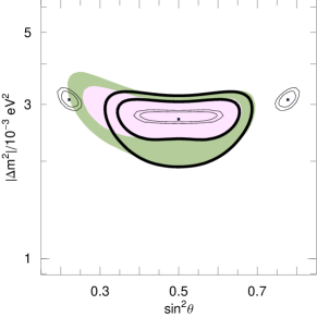
Figure 3: Results of fits to simulated MINOS data with statistics increased from the current $0.93\cdot 10^{20}$ to $25\cdot 10^{20}$ protons on target (thin contours). 90% and 99% C.L. regions are shown. The “data” were simulate for two sets of NSI and “true” oscillation parameters: (i) no NSI, $\sin^{2}\theta=0.5$ and $\Delta m^{2}=2.7\mathrel{{\cdot 10^{-3}~{}{\rm eV^{2}}}}$, (ii) $\mathrel{{\epsilon_{ee}}}=0$, $\mathrel{{\epsilon_{\tau\tau}}}=0.81$, $\mathrel{{\epsilon_{e\tau}}}=0.9$, $\sin 2\theta=0.27$ and $\Delta m^{2}=3.1\mathrel{{\cdot 10^{-3}~{}{\rm eV^{2}}}}$. The fits were done in both cases in the assumption of no NSI. For reference, we also show the regions allowed currently by all the data combined, at 90% and 99% C.L. with (filled area) and without NSI (thick contours), as in Fig. 1. See text for details.

IV NSI-driven $\nu_{\mu}\rightarrow\nu_{e}$ conversion at MINOS

So far, we have discussed the dominant $\nu_{\mu}\rightarrow\nu_{\tau}$ oscillation mode and argued that the effects of intervening matter on this mode are subdominant. We next show that for the $\nu_{\mu}\rightarrow\nu_{e}$ mode matter effects due to NSI can be instead very important. This opens up another, complementary mode for searching for NSI at MINOS.

The $\nu_{\mu}\rightarrow\nu_{e}$ mode is being studied by MINOS as a way to measure/constrain the $\theta_{13}$ mixing angle. According to the analysis by the collaboration, with the planned higher statistics MINOS will have an impressive sensitivity to $\theta_{13}$ in this mode, providing a significant improvement over the current CHOOZ bound. For instance, with $25\times 10^{20}$ protons on target and assuming $\Delta m_{23}=2.5\times 10^{-3}$ eV² the MINOS bound is projected to be $\sin^{2}2\theta_{13}\lesssim 0.07$, compared to $\sin^{2}2\theta_{13}\lesssim 0.14$ as currently given by CHOOZ.

If the non-standard flavor changing interaction $\epsilon_{e\tau}$ is present, it will also drive $\nu_{\mu}\rightarrow\nu_{e}$ conversion. Schematically, this conversion can be viewed in two steps:

$$\nu_{\mu}\stackrel{{\scriptstyle\Delta_{23},\theta_{23}}}{{\longrightarrow}}\nu_{\tau}\stackrel{{\scriptstyle\epsilon_{e\tau}}}{{\longrightarrow}}\nu_{e}.$$ (10)

The first step has already been observed by MINOS, with the largest conversion happening in the lower energy part of its spectrum ($1.5-2$ GeV). Correspondingly, the $\nu_{e}$ production according to Eq. (10) is also expected to peak at low energy. Below, we quantify this by giving an approximate analytical expression for the probability $P(\nu_{\mu}\rightarrow\nu_{e})$ and presenting a sample numerical calculation.

IV.1 Analytical treatment of $\nu_{\mu}\rightarrow\nu_{e}$ conversion

We begin by noting that the probability $P(\nu_{\mu}\rightarrow\nu_{e})$ will be small $(\ll 1)$. This will allow us to treat the process perturbatively. To introduce the idea, let us first consider a toy example. Suppose we have a two-level problem with the Hamiltonian

$$H_{2\nu}=\begin{pmatrix}\delta_{1}&\delta_{12}\\ \delta_{12}&\delta_{2}\end{pmatrix}$$

and the initial state is $(0,1)^{T}$. Assume further that $|\delta_{12}|\ll|\delta_{2}-\delta_{1}|$. Then the probability $P(2\rightarrow 1)$ can be computed in perturbation theory as

$$P(2\rightarrow 1) \simeq \left|\int_{0}^{t}dt^{\prime}(-i)\delta_{12}e^{-i(\delta_{2}-\delta_{1})t^{\prime}}\right|^{2}$$ (11)

$$= \left|\delta_{12}\frac{1-e^{-i(\delta_{2}-\delta_{1})t}}{(\delta_{2}-\delta_{1})}\right|^{2}.$$

To arrive at this one can (i) subtract $\delta_{1}$ on the diagonal (overall constants on the diagonal do not change oscillation probabilities), (ii) solve the evolution equation for $\nu_{2}$ neglecting the effects of $\nu_{1}$, $i\partial_{t}\psi_{2}\simeq(\delta_{2}-\delta_{1})\psi_{2}$, and finally (iii) solve the equation for $\nu_{1}$ treating $\nu_{2}$ obtained before as a source, $i\partial_{t}\psi_{1}=\delta_{12}\psi_{2}$. The second step is the one containing an approximation, it assumes that $|(\delta_{2}-\delta_{1})\psi_{2}|\gg|\delta_{12}\psi_{1}|$.

It is useful to compare Eq. (11) with the exact solution,

$$P(2\rightarrow 1)=\left|\delta_{12}\frac{1-e^{-i\sqrt{(\delta_{2}-\delta_{1})^{2}+4\delta_{12}^{2}}t}}{\sqrt{(\delta_{2}-\delta_{1})^{2}+4\delta_{12}^{2}}}\right|^{2}.$$ (12)

This explicitly shows that (11) is a good approximation so long as $(\delta_{2}-\delta_{1})^{2}\gg 4\delta_{12}^{2}$.

Next, consider a three-level problem with

$$H_{3\nu}=\begin{pmatrix}0&\delta_{12}&\delta_{13}\\ \delta_{12}&\Delta_{2}&0\\ \delta_{13}&0&\Delta_{1}\end{pmatrix}$$

Notice that the 23 block has a diagonal form. Suppose the initial state is $\nu_{23}\equiv(0,a,b)^{T}$ and we again want the probability of finding the particle in the first state. If the off-diagonal entries in this Hamiltonian are smaller than the diagonal ones, we can generalize the previous method to give

$$P(\nu_{23}\rightarrow 1) \simeq \left|(-i)\int_{0}^{t}dt^{\prime}[a\delta_{12}e^{-i\Delta_{2}t^{\prime}}+b\delta_{13}e^{-i\Delta_{1}t^{\prime}}]\right|^{2}$$ (13)

$$= \left|a\delta_{12}\frac{1-e^{-i\Delta_{2}t}}{\Delta_{2}}+b\delta_{13}\frac{1-e^{-i\Delta_{1}t}}{\Delta_{1}}\right|^{2}.$$

The problem we are interested in, that of $\nu_{\mu}\rightarrow\nu_{\tau}\rightarrow\nu_{e}$ conversion, can be reduced to the last case. For that, we need to diagonalize the $\nu_{\mu}-\nu_{\tau}$ block of the Hamiltonian. This is done by rotating this block by an angle $\theta_{23}^{\prime}$ given by

$$\tan 2\theta_{23}^{\prime} = \frac{\Delta\sin 2\theta_{23}}{\Delta\cos 2\theta_{23}+\sqrt{2}G_{F}N_{e}\epsilon_{\tau\tau}/2}.$$ (14)

Notice that this angle is modified from its standard value $\theta_{23}$ by the presence of the NSI matter term.

The two relevant mass splittings are

$$\Delta_{1,2}\simeq\frac{1}{2}\left(\sqrt{2}G_{F}N_{e}\epsilon_{\tau\tau}\pm\sqrt{(\sqrt{2}G_{F}N_{e}\epsilon_{\tau\tau})^{2}+4(\Delta^{2}+\sqrt{2}G_{F}N_{e}\epsilon_{\tau\tau}\Delta\cos 2\theta_{23})}\right)+\Delta-\sqrt{2}G_{F}N_{e}(1+\epsilon_{ee}),$$ (15)

where $\Delta_{1}$ comes with the “+” sign. Normal hierarchy is assumed for definiteness. The small solar splitting is neglected.

The state $\nu_{\mu}$ is a linear combination of the new basis states; correspondingly, the initial wavefunctions are given by $a=\cos\theta_{23}^{\prime}$ and $b=-\sin\theta_{23}^{\prime}$ in the rotated basis. We also need to rotate the NSI $\epsilon_{e\tau}$ term and the vacuum $\theta_{12}$ and $\theta_{13}$ terms. It is important to stress that the $\epsilon_{e\tau}$ term is rotated from the flavor basis (by the angle $\theta_{23}^{\prime}$), while the other two are rotated from the standard (no NSI) basis that diagonalizes the 23 block (by the angle $\theta_{23}^{\prime}-\theta_{23}$).

Combining these ingredients, we finally obtain

$$P(\nu_{\mu}\rightarrow\nu_{e}) \simeq \left|G_{1}\sin\theta_{23}^{\prime}\frac{\exp(i\Delta_{1}L)-1}{\Delta_{1}}-G_{2}\cos\theta_{23}^{\prime}\frac{\exp(i\Delta_{2}L)-1}{\Delta_{2}}\right|^{2},$$ (16)

where

$$G_{1} = \sqrt{2}G_{F}N_{e}\epsilon_{e\tau}\cos\theta_{23}^{\prime}+\Delta\sin 2\theta_{13}\cos(\theta_{23}^{\prime}-\theta_{23})+\Delta_{\odot}\sin 2\theta_{12}\sin(\theta_{23}^{\prime}-\theta_{23}),$$ (17)

$$G_{2} = \sqrt{2}G_{F}N_{e}\epsilon_{e\tau}\sin\theta_{23}^{\prime}+\Delta\sin 2\theta_{13}\sin(\theta_{23}^{\prime}-\theta_{23})-\Delta_{\odot}\sin 2\theta_{12}\cos(\theta_{23}^{\prime}-\theta_{23}).$$ (18)

IV.2 Sample numerical calculation of $\nu_{\mu}\rightarrow\nu_{e}$ conversion

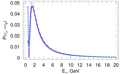
Figure 4: Conversion probability $P(\nu_{\mu}\rightarrow\nu_{e})$ as a function of energy for (i) $\sin^{2}2\theta_{13}=0.07$, $\Delta m_{23}=2.5\times 10^{-3}$ eV², $\sin^{2}\theta_{23}=1/2$ and standard neutrino interactions (short-dashed curve), vs. (ii) $\sin^{2}2\theta_{13}=0$, $\Delta m_{23}=2.9\times 10^{-3}$ eV², $\sin^{2}\theta_{23}=0.36$ and $\epsilon_{ee}=0$, $\epsilon_{e\mu}=0.9$, $\epsilon_{\tau\tau}=0.81$ (solid curve). Both curves were computed numerically. For comparison, the predictions of the analytical result, Eqs. (16,17,18), for the case (ii) are also shown (long-dashed curve).

We are now ready to explore the sensitivity of the $\nu_{\mu}\rightarrow\nu_{e}$ conversion mode to NSI quantitatively. As already mentioned, the MINOS experiment expects to extend the lower bound on $\theta_{13}$ down to $\sin^{2}2\theta<0.07$. We plot the corresponding probability $P(\nu_{\mu}\rightarrow\nu_{e})$ for this case in Fig. 4 (short-dashed curve). We also plot the case with $\theta_{13}=0$ and values of NSI designed to imitate the same effect: $\epsilon_{ee}=0$, $\epsilon_{e\mu}=0.9$, $\epsilon_{\tau\tau}=0.81$ (solid curve). Notice that the epsilons were chosen to lie in the presently allowed region, by satisfying Eq. (5). The details of the parameters are given in the Figure caption.

The Figure shows that the two cases, while quite different for $E_{\nu}<1$ GeV, give indistinguishable signals for $E_{\nu}>1$ GeV, the relevant energy range for MINOS. This fact, already described in Huber et al. (2002a) in the context of neutrino factories, means that the 3$\sigma$ bound expected for $\theta_{13}$ could be translated into a corresponding bound on the NSI.

Our analytical results agree very well with those of the exact numerical calculations. This can be seen in Fig. 4, where the long-dashed curve shows $P(\nu_{\mu}\rightarrow\nu_{e})$ computed according to Eqs. (16,17,18) for the same choice of parameters as the solid curve discussed above. The agreement between the two is more than adequate.

IV.3 Discussion: degeneracy of $\theta_{13}$ and NSI effects; implications for bounds

So far we have shown that the NSI are constrained under the assumption $\theta_{13}=0$. The situation is more complicated if the effects of NSI and $\theta_{13}$ are comparable. It is easy to see from Eqs. (16,17,18) that the two can interfere. The interference can be either constructive or destructive, depending on the relative phases of $\epsilon_{e\tau}$ and $e^{i\delta}\sin 2\theta$. Thus, a non-observation of the $\nu_{\mu}\rightarrow\nu_{e}$ conversion mode at MINOS strictly speaking would not give a simple bound on $\theta_{13}$ or $\epsilon_{e\tau}$, but would define an allowed region in the $e^{i\delta}\sin 2\theta_{13}$ – $\epsilon_{e\tau}$ parameter space. The degeneracy would have to broken by some other means.

IV.4 Note on MINOS baseline advantage over K2K

Finally, we note that MINOS, with its three times longer baseline, possesses an important advantage in sensitivity to the NSI relative to K2K. Indeed, consider Eqs. (16,17,18) and suppose that both the baseline $L$ and the neutrino energy $E_{\nu}$ ($\Delta\propto 1/E_{\nu}$) are varied in such a way that for shorter baseline the oscillation phase in the $\nu_{\nu}\rightarrow\nu_{\tau}$ channel is preserved. It is then clearly seen that the matter term, $\propto\sqrt{2}G_{F}N_{e}\epsilon_{e\tau}$, becomes relatively less important than the vacuum oscillation term driven by $\theta_{13}$, $\propto\Delta\sin 2\theta_{13}$. Thus, the K2K experiment is less sensitive to the NSI than MINOS. The published K2K bound $\sin^{2}2\theta_{13}<0.26$ at 90% C.L. Yamamoto et al. (2006) does not translate in any useful bound on the NSI parameter space, as we have checked both analytically and numerically.

V Summary

We have presented the results of a combined analysis of the data from atmospheric neutrinos at SuperKamiokande, K2K and MINOS, performed to test neutrino nonstandard interactions. The focus has been on the effect of adding the recent MINOS data to the analysis of the atmospheric and K2K data.

We find that the allowed region in the space of the parameters $\sin^{2}\theta,\Delta m^{2},\mathrel{{\epsilon_{ee}}},\mathrel{{\epsilon_{\tau\tau}}},\mathrel{{\epsilon_{e\tau}}}$ has the shape predicted by the analytics (and confirmed by the data analysis before the MINOS data Friedland and Lunardini (2005)): it has a parabolic direction in the space of the NSI couplings and extends to smaller $\theta$ and larger $\mathrel{{\Delta m^{2}}}$ with respect to the region found without NSI. With the addition of MINOS, the region becomes narrower but the part of the region at small $\theta$ due to NSI remains allowed, see Fig. 1.

Another effect of MINOS is to shift the best fit point to non-zero NSI, mixing smaller than maximal, and slightly larger $\mathrel{{\Delta m^{2}}}$. However, there is only an insignificant difference in $\chi^{2}$ between the best fit point and the point that minimizes the $\chi^{2}$ for zero NSI.

Much stronger conclusions could be obtained in the future, when MINOS has higher statistics. Here we have shown examples of fits to simulated MINOS data with $\simeq 27$ times larger statistics (“MINOS-high” sample) combined with the atmospheric and K2K data as they are today (no updates are expected from K2K, which is now closed). We find that in this scenario the precision is sufficient to reveal oscillation parameters in tension with the analysis of atmospheric neutrinos in absence of NSI, and thus to give an indication of the existence of new interactions. It is possible that the point $\mathrel{{\epsilon_{ee}}}=\mathrel{{\epsilon_{e\tau}}}=\mathrel{{\epsilon_{\tau\tau}}}=0$ will be outside the 99% C.L. region of the combined analysis of all the data. This requires a significant shift of the vacuum parameters with respect to the matter ones, $\theta_{m}$ and $\Delta m^{2}_{m}$, corresponding to a large “matter” angle, $\beta$, $\beta\mathrel{\vbox{\hbox{$>$}\nointerlineskip\hbox{$\sim$}}}0.3\pi$ (see Eq. (8)). Such condition typically corresponds to $|\mathrel{{\epsilon_{e\tau}}}|\mathrel{\vbox{\hbox{$>$}\nointerlineskip\hbox{$\sim$}}}0.5$ per electron, i.e. NSI per quark at the level of $\sim 10\%$ of the Standard Model interaction.

It should be considered that, since the sensitivity to NSI arises from combining data from a neutrino beam like MINOS and the signal from atmospheric neutrinos, the latter may become the limiting factor as the precision of the beam measurements increases. This should motivate a second phase in the study of atmospheric neutrino oscillations, characterized by higher precision, desirably of the same level – $\sim 10-20\%$ – of the perspective MINOS precision. Such second phase could be realized at Megaton water Cherenkov detectors like UNO Jung (2000); Wilkes (2005), HyperKamiokande Nakamura (2003) and MEMPHYS Mosca (2005). Alternatively, the presence of NSI could be revealed by the combination of high precision measurements from different beam experiments. A typical scenario would require two beams of different baseline, one of similar length as MINOS and the other with a baseline longer by a factor of several. For this second beam the matter width would be sufficient to have significant refraction effects, if the epsilons are close to $\sim 1$ (per electron, meaning about 0.2 per $u$ and $d$ quarks). This long baseline experiment would play the same role played by atmospheric neutrinos in this paper. Finally, a third possibility to test for NSI is to use a MINOS-like beam to look at oscillation channels where vacuum oscillations would be suppressed by the smallness of the mixing $\theta_{13}$ rather than by the high energy, so that small effects of NSI would not be hidden by larger vacuum oscillation effects as it happens for part of the atmospheric neutrino spectrum.

We have investigated the latter possibility for the case of MINOS-high. The main finding is that epsilons of order unity could give a measurable $\mathrel{{\nu_{\mu}}}-\mathrel{{\nu_{e}}}$ conversion probability of the order of few $10^{-2}$. In the interval of energy relevant for MINOS the NSI-induced signal for $\theta_{13}=0$ can mimic the effect of $\theta_{13}$ (with no NSI), and vice versa. To break the degeneracy between the two scenarios would require a combination of tests in several oscillation channels at a neutrino beam like MINOS itself, or a quasi-vacuum test of $\mathrel{{\nu_{\mu}}}-\mathrel{{\nu_{e}}}$ conversion, of the type planned for nuclear reactor experiments, e.g. Ardellier et al. (2004).

Finally, we again stress the importance of measuring the neutral current event rate in the MINOS far detector, as a complementary mode for searching for the NSI. Since the flux at the far detector contains a significant $\nu_{\tau}$ component, such a measurement would be a valuable probe of new tau neutrino interactions. This probe would be complementary to the matter effects considered here, because the cross-section effects are sensitive to, in general, different combinations of the NSI as discussed in Friedland and Lunardini (2005) . Such an analysis would be a generalization of the search for the sterile neutrino component already planned by the MINOS collaboration.

In conclusion, we have shown that the potential of MINOS goes beyond confirming and adding precision to the already accepted $\mathrel{{\nu_{\mu}}}\rightarrow\mathrel{{\nu_{\tau}}}$ vacuum oscillations scenario that explains atmospheric neutrinos data, and testing vacuum oscillations in the $\mathrel{{\nu_{\mu}}}-\mathrel{{\nu_{e}}}$ channel. This experiment can be a valuable tool to search for exotic neutrino-matter interactions, both in the $\mathrel{{\nu_{\mu}}}$ disappearance and in the $\mathrel{{\nu_{e}}}$ appearance parts of its program, and this should motivate its long term operation into a phase of precision measurements. Our study also makes a general point, that it is important to test neutrino oscillations with high precision both in environments where matter effects are suppressed and in cases with strong matter effects, because the comparison of the two could reveal new physics. This motivates higher precision measurements with atmospheric neutrinos and contributes to make the case for long baseline neutrino beams and for a new generation of reactor neutrino experiments.

Acknowledgments

We are especially grateful to Michele Maltoni for providing the numerical executable used in our past work Friedland and Lunardini (2005), the results of which were used in the present paper. A.F. was supported by the Department of Energy, under contract number DE-AC52-06NA25396. C.L. acknowledges support from the INT-SCiDAC grant number DE-FC02-01ER41187.

Note added

While the text of this work was being finalized, the paper by Kitazawa, Sugiyama and Yasuda Kitazawa et al. (2006) appeared online, discussing ideas similar to ours about testing NSI in the $\mathrel{{\nu_{\mu}}}-\mathrel{{\nu_{e}}}$ channel at MINOS. Our work adds to theirs the three neutrinos analytical formalism, helpful to analyze the $\theta_{13}-\mathrel{{\epsilon_{e\tau}}}$ degeneracy.

References

- Vilain et al. (1994) P. Vilain et al. (CHARM-II), Phys. Lett. B335, 246 (1994).
- Zeller et al. (2002) G. P. Zeller et al. (NuTeV), Phys. Rev. Lett. 88, 091802 (2002), eprint hep-ex/0110059.
- Berezhiani and Rossi (2002) Z. Berezhiani and A. Rossi, Phys. Lett. B535, 207 (2002), eprint hep-ph/0111137.
- Davidson et al. (2003) S. Davidson, C. Pena-Garay, N. Rius, and A. Santamaria, JHEP 03, 011 (2003), eprint hep-ph/0302093.
- Fornengo et al. (2002) N. Fornengo, M. Maltoni, R. T. Bayo, and J. W. F. Valle, Phys. Rev. D65, 013010 (2002), eprint hep-ph/0108043.
- Guzzo et al. (2002) M. Guzzo et al., Nucl. Phys. B629, 479 (2002), eprint hep-ph/0112310.
- Gonzalez-Garcia and Maltoni (2004) M. C. Gonzalez-Garcia and M. Maltoni, Phys. Rev. D70, 033010 (2004), eprint hep-ph/0404085.
- Friedland et al. (2004a) A. Friedland, C. Lunardini, and C. Pena-Garay, Phys. Lett. B594, 347 (2004a), eprint hep-ph/0402266.
- Friedland et al. (2004b) A. Friedland, C. Lunardini, and M. Maltoni, Phys. Rev. D70, 111301 (2004b), eprint hep-ph/0408264.
- Friedland and Lunardini (2005) A. Friedland and C. Lunardini, Phys. Rev. D72, 053009 (2005), eprint hep-ph/0506143.
- Ahn et al. (2003) M. H. Ahn et al. (K2K), Phys. Rev. Lett. 90, 041801 (2003), eprint hep-ex/0212007.
- Aliu et al. (2005) E. Aliu et al. (K2K), Phys. Rev. Lett. 94, 081802 (2005), eprint hep-ex/0411038.
- Adamson et al. (2006) P. Adamson et al. (MINOS), Phys. Rev. D73, 072002 (2006), eprint hep-ex/0512036.
- Petyt (2006) D. Petyt (MINOS), talk given at FNAL, available at http://wwwnumi.fnal.gov/talks/results06.html. (2006).
- Gago et al. (2001) A. M. Gago, M. M. Guzzo, H. Nunokawa, W. J. C. Teves, and R. Zukanovich Funchal, Phys. Rev. D64, 073003 (2001), eprint hep-ph/0105196.
- Huber et al. (2002a) P. Huber, T. Schwetz, and J. W. F. Valle, Phys. Rev. Lett. 88, 101804 (2002a), eprint hep-ph/0111224.
- Campanelli and Romanino (2002) M. Campanelli and A. Romanino, Phys. Rev. D66, 113001 (2002), eprint hep-ph/0207350.
- Blennow et al. (2005) M. Blennow, T. Ohlsson, and W. Winter (2005), eprint hep-ph/0508175.
- Huber et al. (2002b) P. Huber, T. Schwetz, and J. W. F. Valle, Phys. Rev. D66, 013006 (2002b), eprint hep-ph/0202048.
- Apollonio et al. (1999) M. Apollonio et al. (CHOOZ), Phys. Lett. B466, 415 (1999), eprint hep-ex/9907037.
- Apollonio et al. (2003) M. Apollonio et al., Eur. Phys. J. C27, 331 (2003), eprint hep-ex/0301017.
- Friedland and Lunardini (2003) A. Friedland and C. Lunardini, Phys. Rev. D68, 013007 (2003), eprint hep-ph/0304055.
- Engel et al. (2000) R. Engel, T. K. Gaisser, and T. Stanev, Phys. Lett. B472, 113 (2000), eprint hep-ph/9911394.
- Lunardini and Smirnov (2000) C. Lunardini and A. Y. Smirnov, Nucl. Phys. B583, 260 (2000), eprint hep-ph/0002152.
- Hayato (2004) Y. Hayato, Eur. Phys. J. C33, s829 (2004).
- Ashie et al. (2005) Y. Ashie et al. (Super-Kamiokande), Phys. Rev. D71, 112005 (2005), eprint hep-ex/0501064.
- Yamamoto et al. (2006) S. Yamamoto et al. (K2K), Phys. Rev. Lett. 96, 181801 (2006), eprint hep-ex/0603004.
- Jung (2000) C. K. Jung, AIP Conf. Proc. 533, 29 (2000), eprint hep-ex/0005046.
- Wilkes (2005) R. J. Wilkes (2005), eprint hep-ex/0507097.
- Nakamura (2003) K. Nakamura, Int. J. Mod. Phys. A18, 4053 (2003).
- Mosca (2005) L. Mosca, Nucl. Phys. Proc. Suppl. 138, 203 (2005).
- Ardellier et al. (2004) F. Ardellier et al. (2004), eprint hep-ex/0405032.
- Kitazawa et al. (2006) N. Kitazawa, H. Sugiyama, and O. Yasuda (2006), eprint hep-ph/0606013.