New gauge boson $B_{H}$ production associated with W boson pair via $\gamma\gamma$ collision in the littlest Higgs model

Abstract

The littlest Higgs model is the most economical little Higgs model. The observation of the new gauge bosons predicted by the littlest Higgs model could serve as a robust signature of the model. The ILC, with the high energy and luminosity, can open an ideal window to probe these new gauge bosons, specially, the lightest $B_{H}$. In the framework of the littlest Higgs model, we study a gauge boson $B_{H}$ production process $\gamma\gamma\rightarrow W^{+}W^{-}B_{H}$. The study shows that the cross section of the process can vary in a wide range($10^{-1}-10^{1}$ fb) in most parameter spaces preferred by the electroweak precision data. The high c.m. energy(For example, $\sqrt{s}=1500$ GeV) can obviously enhance the cross section to the level of tens fb. For the favorable parameter spaces, the sufficient typical events could be assumed at the ILC. Therefore, our study about the process $\gamma\gamma\rightarrow W^{+}W^{-}B_{H}$ could provide a useful theoretical instruction for probing $B_{H}$ experimentally at ILC. Furthermore, such process would offer a good chance to study the triple and quartic gauge couplings involving $B_{H}$ and the SM gauge bosons which shed important light on the symmetry breaking features of the littlest Higgs model.

PACS number(s): 12.60Nz,14.80.Mz,12.15.Lk,14.65.Ha

1 Introduction

At present the success of the standard model(SM) is well known and doubtless. However, the mechanism of electroweak symmetry breaking(EWSB) remains the most prominent mystery in current particle physics. The Higgs particle that is assumed to trigger the EWSB in the SM has not been found. In addition, there are prominent problems of triviality and unnaturalness in the Higgs sector. Thus, the SM can only be an excellent effective field theory below some high energy scales. New physics beyond the SM should exist at the TeV scale. The possible new physics scenarios at the TeV scale might be supersymmetry(SUSY)[1], dynamical symmetry breaking[2], extra dimensions[3], the little Higgs model [4, 5, 6, 7] etc.

Among the extended models beyond the SM, the little Higgs model offers a very promising solution to the hierarchy problem in which the Higgs boson is naturally light as a result of nonlinearly realized symmetry. The key feature of this model is that the Higgs boson is a pseudo-Goldstone boson of an approximate global symmetry which is spontaneously broken by a vacuum expectation value(vev) at a scale of a few TeV and thus is naturally light. Such model can be regarded as the important candidate of new physics beyond the SM. The littlest Higgs model [7] is a simplest and phenomenologically viable model to realizes the little Higgs idea. The model predicts the presence of the new gauge bosons $(B_{H},Z_{H},W^{\pm}_{H})$ and their masses are in the range of a few TeV, except for $B_{H}$ in the range of hundreds of GeV. The minimality of the littlest Higgs model would leave the characteristic signatures at present and future high energy collider experiments.

It is widely believed that the hadron colliders, such as the Tevatron and the LHC running in 2007, can directly probe the possible new physics beyond the SM up to a few TeV, while the TeV energy linear $e^{+}e^{-}$ collider(LC) is also required to complement the probe of the new particles with detailed measurements[8]. A unique feature of the TeV energy LC is that it can be transformed to $\gamma\gamma$ or $e\gamma$ collider(the photon collider) by the laser-scattering method. In this case the energy and luminosity of the photon beams would be the same order of magnitude of the original electron beams and the set of final states at the photon collider is much rich than that in the $e^{+}e^{-}$ mode. Furthermore, one can vary polarizations of photon beams relatively easily, which is advantageous for experiments. In some scenarios, the photon collider is the best instrument for the discovery of the signals of the new physics models and will be able to study multiple vector boson production with high precision.

The probe of the new particles, specially the new gauge bosons predicted by the littlest Higgs model, can provide a direct way to test the model. The CERN Large Hadronic Collider(LHC), with the center of energy $\sqrt{s}=14$ TeV, has the ability to produce these heavy new particles. In some literatures[9, 10], the production mechanism of these new particles at the LHC has been studied and the most promising production process is Drell-Yan process which shows that the LHC has the potential to detect them. However, the detailed study of these new gauge boson couplings needs the precision measurement at the future LC, and such work can be performed at the planned International Linear Collider(ILC) with the center of mass(c.m.) energy $\sqrt{s}$=300 GeV-1.5 TeV and the yearly luminosity 500 $fb^{-1}$[11]. Specially for the gauge boson $B_{H}$, we find that the global symmetry structure $SU(5)/SO(5)$ of the littlest Higgs model allows a substantially light $B_{H}$ with the mass about a few hundred GeV, and such gauge boson is light enough to be produced at the first running of the ILC. Therefore, the exploring of this light $B_{H}$ at the ILC would play an important role in testing the littlest Higgs model. Some phenomenological studies of littlest Higgs model via $e^{+}e^{-}$ collision at the ILC has been done[12]. The ILC has the capability to discover the effects of the littlest Higgs model over the entire theoretically interesting range of parameters and to determine the couplings of the heavy gauge bosons to the precision of a few percent. The realization of $\gamma\gamma$ collision would provide us a better chances to probe $B_{H}$. In this paper, we study a $B_{H}$ production process associated with W boson pair via $\gamma\gamma$ collision realized at the ILC, i.e., $\gamma\gamma\rightarrow W^{+}W^{-}B_{H}$. The motivation to study this process is that $W^{+}W^{-}B_{H}$ production mode can be realized below the TeV scale and its cross section is large enough to detect $B_{H}$ with the high energy and luminosity of the ILC. On the other hand, such process offers a direct study of vector boson couplings in the littlest Higgs model.

This paper is organized as follows. In the section two, we briefly review the littlest Higgs model. In the section three, the calculation process of the cross section is presented. The section four contains our numerical results and conclusions.

2 Brief review of the littlest Higgs model

The minimal model containing the little Higgs ideas is called the littlest Higgs model. This model is based on a non-linear sigma model and consists of a global $SU(5)$ symmetry which is broken down to $SO(5)$ by a vacuum condensate $f\sim\frac{\Lambda_{s}}{4\pi}\sim$ TeV which results in 14 Goldstone bosons. The effective field theory of those Goldstone bosons is parameterized by a non-linear $\sigma$-model with a gauge symmetry $[SU(2)\times U(1)]^{2}$. The breaking of the global $SU(5)$ down to $SO(5)$ simultaneously breaks $[SU(2)\times U(1)]^{2}$ down to its diagonal $SU(2)_{L}\times U(1)_{Y}$ subgroup, which is identified as the SM electroweak gauge group. In particular, the Lagrangian will still preserve the full $[SU(2)\times U(1)]^{2}$ gauge symmetry.

The leading order dimension-two term in the non-linear $\sigma$-model can be written for the scalar sector as

$${\pounds}_{\Sigma}=\frac{f^{2}}{8}Tr|D_{\mu}\Sigma|^{2},$$ (1)

with the covariant derivative

$$D_{\mu}\Sigma=\partial_{\mu}\Sigma-i\sum^{2}_{j=1}[g_{j}(W_{j}\Sigma+\Sigma W^{T}_{j})+g^{\prime}_{j}(B_{j}\Sigma+\Sigma B^{T}_{j})].$$ (2)

Where $W_{j}=\sum^{3}_{a=1}W^{a}_{\mu j}Q^{a}_{j}$ and $B_{j}=B_{\mu j}Y_{j}$ are the $SU(2)$ and $U(1)$ gauge fields, respectively. The low-energy dynamics is described in term of the non-linear sigma model field

$$\Sigma(x)=e^{2i\Pi/f}\Sigma_{0},$$ (3)

where $\Pi=\sum_{a}\pi^{a}(x)X^{a}$. The sum runs over the 14 broken $SU(5)$ generators $X^{a}$, and $\pi^{a}(x)$ are the Goldstone bosons. The symmetry breaking vev is proportional to $\Sigma_{0}$.

The gauge boson mass eigenstates after the spontaneous gauge symmetry breaking are

$$W=sW_{1}+cW_{2},~{}~{}~{}~{}W^{\prime}=-cW_{1}+sW_{2},$$ (4)

$$B=s^{\prime}B_{1}+c^{\prime}B_{2},~{}~{}~{}~{}B^{\prime}=-c^{\prime}B_{1}+s^{\prime}B_{2}.$$ (5)

$s,c,s^{\prime},c^{\prime}$ are mixing angles and are defined as

$$s\equiv sin\psi=\frac{g_{2}}{\sqrt{g^{2}_{1}+g^{2}_{2}}},~{}~{}~{}~{}s^{\prime}\equiv sin\psi^{\prime}=\frac{g^{\prime}_{2}}{\sqrt{g^{\prime 2}_{1}+g^{\prime 2}_{2}}},$$ (6)

$$c\equiv cos\psi=\sqrt{1-s^{2}},~{}~{}~{}~{}c^{\prime}\equiv cos\psi^{\prime}=\sqrt{1-s^{\prime 2}}.$$ (7)

The $W$ and $B$ remain massless and are identified as the SM gauge bosons, with couplings

$$g=g_{1}s=g_{2}c,\ \ \ g^{\prime}=g^{\prime}_{1}s^{\prime}=g^{\prime}_{2}c^{\prime}.$$ (8)

$W^{\prime}$ and $B^{\prime}$ are the heavy the massive gauge bosons associated with the four broken generators of $[SU(2)\times U(1)]^{2}$.

After linearize the theory, the couplings of the gauge bosons to Higgs field can be obtained via Eq.(1) at leading order in $1/f$

$$\frac{1}{4}H[g^{2}(W^{\mu a}W^{a}_{\mu}-W^{\prime\mu a}W^{\prime a}_{\mu}-2cot2\psi W^{\prime\mu a}W^{a}_{\mu})+g^{\prime 2}(B^{\mu}B_{\mu}-B^{\prime\mu}B^{\prime}_{\mu}-2cot2\psi^{\prime}B^{\prime\mu}B_{\mu})]H^{{\dagger}}.$$ (9)

where $H=(h^{+},h_{0})$ is the SM Higgs doublet.

In the SM, the four-point couplings of the form $W^{a}_{\mu}W^{\mu a}H^{\dagger}H$ and $B_{\mu}B^{\mu}H^{\dagger}H$ lead to a quadratically divergent in the Higgs mass arising from the seagull diagrams involving gauge boson loops. From Eq(9), we can see that, in the littlest Higgs model, the $W^{\prime a}_{\mu}W^{\prime\mu a}H^{\dagger}H$ and $B^{\prime}_{\mu}B^{\prime\mu}H^{\dagger}H$ couplings have unusual forms which serves to exactly cancel the quadratic divergence in the Higgs mass leaded by $W^{a}_{\mu}W^{\mu a}H^{\dagger}H$ and $B_{\mu}B^{\mu}H^{\dagger}H$. The cancellation of such divergence is a crucial feature of the little Higgs theory. The key test of the little Higgs mechanism in the gauge sector is the experimental verification of this feature. Some literatures have discussed the prospects at the LHC[10].

The EWSB in the littlest Higgs model is triggered by the Higgs potential generated by one-loop radiative correction and massless $W$ and $B$ obtain their masses. The Higgs potential includes the parts generated by the gauge boson loops as well as the the fermion loops.

The EWSB induces further mixing between the light and heavy gauge bosons and the final observed mass eigenstates are the light SM-like bosons $W_{L}^{\pm},Z_{L}$ and $A_{L}$ observed in experiment, and new heavy bosons $W^{\pm}_{H},Z_{H}$ and $B_{H}$ that could be observed in future experiments. The masses of neutral gauge bosons are given to $O(v^{2}/f^{2})$ by[12]

$$M^{2}_{A_{L}} = 0,$$ (10)

$$M^{2}_{Z_{L}} = (M^{SM}_{Z})^{2}\{1-\frac{v^{2}}{f^{2}}[\frac{1}{6}+\frac{1}{4}(c^{2}-s^{2})^{2}+\frac{5}{4}(c^{\prime 2}-s^{\prime 2})^{2}]+8\frac{v^{\prime 2}}{v^{2}}\},$$ (11)

$$M^{2}_{Z_{H}} = (M^{SM}_{W})^{2}\{\frac{f^{2}}{s^{2}c^{2}v^{2}}-1+\frac{v^{2}}{2f^{2}}[\frac{(c^{2}-s^{2})^{2}}{2c_{W}^{2}}+\chi_{H}\frac{g^{\prime}}{g}\frac{c^{\prime 2}s^{2}+c^{2}s^{\prime 2}}{cc^{\prime}ss^{\prime}}]\},$$ (12)

$$M^{2}_{B_{H}} = (M^{SM}_{Z})^{2}s^{2}_{W}\{\frac{f^{2}}{5s^{\prime 2}c^{\prime 2}v^{2}}-1+\frac{v^{2}}{2f^{2}}[\frac{5(c^{\prime 2}-s^{\prime 2})^{2}}{2s^{2}_{W}}-\chi_{H}\frac{g}{g^{\prime}}\frac{c^{\prime 2}s^{2}+c^{2}s^{\prime 2}}{cc^{\prime}ss^{\prime}}]\}.$$ (13)

Where $\chi_{H}=\frac{5}{2}gg^{\prime}\frac{scs^{\prime}c^{\prime}(c^{2}s^{\prime 2}+s^{2}c^{\prime 2})}{5g^{2}s^{\prime 2}c^{\prime 2}-g^{\prime}s^{2}c^{2}}$, $v$=246 GeV is the elecroweak scale, $v^{\prime}$ is the vev of the scalar $SU(2)_{L}$ triplet and $s_{W}(c_{W})$ represents the sine(cosine) of the weak mixing angle.

On the other hand, the EWSB also induces cubic couplings between the physical Higgs boson and the gauge bosons. The explicit forms of these couplings can be obtained from Eq.(1) after linearizing the theory. The three diagonal coupling, $hZZ,~{}hZ_{H}Z_{H},~{}hB_{H}B_{H}$, add up to zero. So do the two diagonal couplings $hW^{+}W^{-}$ and $hW^{+}_{H}W^{-}_{H}$. These cancellations can be traced back to Eq.(9), and are therefore directly related to the crucial feature of cancellation of quadratic divergences. Measuring the diagonal coupling would provide the most direct way to verify the little Higgs theory. Such measurement requires associated production of a new heavy boson with a Higgs and is a difficult task. However, it is much easier to measure the off-diagonal couplings, such as $hZ_{H}Z,~{}hB_{H}Z,~{}hW^{\pm}_{H}W^{\mp}$. Although these couplings do not directly participate in the cancellation of quadratic divergences, verifying their structure would provide a strong evidence for the crucial feature of the model.

The gauge kinetic terms $\pounds_{G}$ take the standard form:

$$\pounds_{G}=-\frac{1}{4}\sum^{2}_{j=1}(W^{\mu\nu}_{ja}W^{a}_{j\mu\nu}+B^{\mu\nu}_{ja}B^{a}_{j\mu\nu}).$$ (14)

These terms yield 3- and 4-particle interactions among the gauge bosons.

There are still other interactions in the littlest Higgs model, ${\pounds}_{F},{\pounds}_{Y},V_{CW}$. The fermion kinetic terms ${\pounds}_{F}$ can give the couplings of the gauge bosons with fermions. The couplings of the scalars h and $\phi$ with fermions can be derived from the Yukawa interaction terms ${\pounds}_{Y}$. The effective Higgs potential, the Coleman-weinberg potential $V_{CW}$, is generated at one-loop and higher orders due to the interactions of Higgs with gauge bosons and fermions, which can induce the EWSB by driving the Higgs mass squared parameter negative.

It is shown via above discussion that the new heavy gauge bosons $B_{H},Z_{H},W^{\pm}_{H}$ are predicted in the littlest Higgs model and these new particles might produce the characteristic signatures at the present and future high energy collider experiments [9, 10, 12, 13].

3 The cross section of the process $\gamma\gamma\rightarrow W^{+}W^{-}B_{H}$

From the gauge kinetic terms $\pounds_{G}$, one can derive the 3-point and 4-point gauge self-coupling expressions. With all momenta out-going, the 3-point gauge boson self-couplings can be written in form of[9]

$$V_{1}^{\mu}(k_{1})V_{2}^{\nu}(k_{2})V_{3}^{\rho}(k_{3}):~{}~{}-ig_{V_{1}V_{2}V_{3}}[g^{\mu\nu}(k_{1}-k_{2})^{\rho}+g^{\nu\rho}(k_{2}-k_{3})^{\mu}+g^{\rho\mu}(k_{3}-k_{1})^{\nu}],$$ (15)

and the 4-point gauge boson self-couplings take the form

$$W_{1}^{+\mu}W_{2}^{+\nu}W_{3}^{-\rho}W_{4}^{-\sigma}:~{}~{}-ig_{W_{1}^{+}W_{2}^{+}W_{3}^{-}W_{4}^{-}}(2g^{\mu\nu}g^{\rho\sigma}-g^{\mu\rho}g^{\nu\sigma}-g^{\nu\rho}g^{\mu\sigma}),$$ (16)

$$V_{1}^{\mu}V_{2}^{\nu}W_{1}^{+\rho}W_{2}^{-\sigma}:~{}~{}ig_{V_{1}V_{2}W_{1}^{+}W_{2}^{-}}(2g^{\mu\nu}g^{\rho\sigma}-g^{\mu\rho}g^{\nu\sigma}-g^{\nu\rho}g^{\mu\sigma}).$$ (17)

The coefficients $g_{V_{1}V_{2}V_{3}},~{}g_{W_{1}^{+}W_{2}^{+}W_{3}^{-}W_{4}^{-}}$ and $g_{V_{1}V_{2}W_{1}^{+}W_{2}^{-}}$ are given as

$$g_{A_{L}W^{+}_{L}W^{-}_{L}}=-e,\ \ \ g_{W^{+}_{L}W^{-}_{L}B_{H}}=\frac{ec_{W}}{s_{W}}\frac{v^{2}}{f^{2}}x_{Z}^{B^{\prime}},$$ (18)

$$g_{A_{L}A_{L}W^{+}_{L}W^{-}_{L}}=-e^{2},\ \ \ \ g_{A_{L}W^{+}_{L}W^{-}_{L}B_{H}}=\frac{e^{2}c_{W}}{s_{W}}\frac{v^{2}}{f^{2}}x_{Z}^{B^{\prime}}.$$ (19)

Where $x_{Z}^{B^{\prime}}=-\frac{5}{2s_{W}}s^{\prime}c^{\prime}(c^{\prime 2}-s^{\prime 2})$. We can see that the couplings $A_{L}W^{+}_{L}W^{-}_{L}$ and $A_{L}A_{L}W^{+}_{L}W^{-}_{L}$ are just the same as the couplings $\gamma W^{+}W^{-}$ and $\gamma\gamma W^{+}W^{-}$ in the SM. Comparing the mass of $W_{L}$ with the SM $W$, we find there exists a correction term in order of $v^{2}/f^{2}$. Limited by the electroweak precision data, such correction should be much small. So, we can safely regard $A_{L}$ and $W_{L}$ in the littlest Higgs model as $\gamma$ and $W$ in the SM. So, we will represent $A_{L},W_{L}$ as $\gamma,W$ in the following discussion.

Via above 3-point and 4-point gauge self-couplings, the process $\gamma\gamma\rightarrow W^{+}W^{-}B_{H}$ can be realized in the way shown in Fig.1.

The crossing diagrams with the interchange of the two incoming photons are not shown. The initial photons are denoted by $\varepsilon_{\mu}(k_{1})$, $\varepsilon_{\nu}(k_{2})$ and the final state $W^{+},W^{-},B_{H}$ are given by $\varepsilon_{\alpha}(p_{+}),~{}\varepsilon_{\beta}(p_{-}),~{}\varepsilon_{\gamma}(k_{3})$, respectively. The production amplitudes of the process can be written as

$$M = G\cdot\varepsilon_{\mu}(k_{1})\varepsilon_{\nu}(k_{2})\varepsilon_{\alpha}(p_{+})\varepsilon_{\beta}(p_{-})\varepsilon_{\gamma}(k_{3})M^{\mu\nu\alpha\beta\gamma},$$ (20)

with

$$M^{\mu\nu\alpha\beta\gamma} = \sum_{\zeta=a,b,c,d,e,f,g}M_{\zeta}^{\mu\nu\alpha\beta\gamma},$$ (21)

with

$$G=\frac{5}{2}\frac{e^{3}c_{W}}{s_{W}^{2}}\frac{v^{2}}{f^{2}}s^{\prime}c^{\prime}(c^{\prime 2}-s^{\prime 2}).$$ (22)

Where $M_{\zeta}^{\mu\nu\alpha\beta\gamma}$ is the contribution of Fig.1(a-g) to the process.

In order to write a compact expression for the amplitudes, it is convenient to define the triple-boson couplings coefficient as

$$\Gamma_{3}^{\alpha\beta\gamma}(p_{1},p_{2},p_{3}) = g^{\alpha\beta}(p_{1}-p_{2})^{\gamma}+g^{\beta\gamma}(p_{2}-p_{3})^{\alpha}+g^{\gamma\alpha}(p_{3}-p_{1})^{\beta},$$ (23)

with all momenta out-going, the quartic-boson coupling coefficient as

$$\Gamma_{4}^{\mu\nu\alpha\beta} = 2g^{\mu\nu}g^{\alpha\beta}-g^{\mu\alpha}g^{\nu\beta}-g^{\nu\alpha}g^{\mu\beta},$$ (24)

and the W boson propagator tensor

$$D^{\mu\nu}(k) = \frac{g^{\mu\nu}}{k^{2}-M_{W}^{2}}.$$ (25)

Using the above definitions, we can explicitly write $M_{\zeta}^{\mu\nu\alpha\beta\gamma}$ as

$$M_{a}^{\mu\nu\alpha\beta\gamma}=\Gamma_{3}^{\alpha\gamma\xi}(p_{+},k_{3},-p_{+}-k_{3})D_{\xi\sigma}(p_{+}+k_{3})\Gamma_{3}^{\mu\sigma\rho}(-k_{1},p_{+}+k_{3},k_{2}-p_{-})$$ (26)

$$\hskip 48.36958ptD_{\rho\lambda}(p_{-}-k_{2})\Gamma_{3}^{\beta\nu\lambda}(p_{-},-k_{2},p_{-}-k_{2})+[k_{1\leftrightarrow 2};\mu\leftrightarrow\nu],$$

$$M_{b}^{\mu\nu\alpha\beta\gamma}=\Gamma_{3}^{\beta\xi\gamma}(p_{-},-p_{-}-k_{3},k_{3})D_{\xi\sigma}(p_{-}+k_{3})\Gamma_{3}^{\sigma\nu\rho}(p_{-}+k_{3},-k_{2},p_{+}-k_{1})$$

$$\hskip 48.36958ptD_{\rho\lambda}(p_{+}-k_{1})\Gamma_{3}^{\mu\alpha\lambda}(-k_{1},p_{+},k_{1}-p_{+})+[k_{1\leftrightarrow 2};\mu\leftrightarrow\nu],$$

$$M_{c}^{\mu\nu\alpha\beta\gamma}=\Gamma_{3}^{\mu\alpha\xi}(-k_{1},p_{+},k_{1}-p_{+})D_{\xi\sigma}(k_{1}-p_{+})\Gamma_{3}^{\sigma\gamma\rho}(p_{+}-k_{1},k_{3},p_{-}-k_{2})$$

$$\hskip 48.36958ptD_{\rho\lambda}(p_{-}-k_{2})\Gamma_{3}^{\beta\nu\lambda}(p_{-},-k_{2},k_{2}-p_{-})+[k_{1\leftrightarrow 2};\mu\leftrightarrow\nu],$$

$$M_{d}^{\mu\nu\alpha\beta\gamma}=\Gamma_{3}^{\beta\nu\xi}(p_{-},-k_{2},k_{2}-p_{-})D_{\xi\lambda}(k_{2}-p_{-})\Gamma_{4}^{\lambda\alpha\mu\gamma}+[k_{1\leftrightarrow 2};\mu\leftrightarrow\nu],$$

$$M_{e}^{\mu\nu\alpha\beta\gamma}=\Gamma_{3}^{\mu\alpha\xi}(-k_{1},p_{+},k_{1}-p_{+})D_{\xi\lambda}(k_{1}-p_{+})\Gamma_{4}^{\lambda\beta\nu\gamma}+[k_{1\leftrightarrow 2};\mu\leftrightarrow\nu],$$

$$M_{f}^{\mu\nu\alpha\beta\gamma}=\Gamma_{3}^{\alpha\gamma\xi}(p_{+},k_{3},-k_{3}-p_{+})D_{\xi\lambda}(k_{3}+p_{+})\Gamma_{4}^{\lambda\beta\nu\mu},$$

$$M_{g}^{\mu\nu\alpha\beta\gamma}=\Gamma_{3}^{\gamma\beta\xi}(k_{3},p_{-},-k_{3}-p_{-})D_{\xi\lambda}(k_{3}+p_{-})\Gamma_{4}^{\lambda\alpha\nu\mu}.$$

Where $[k_{1\leftrightarrow 2};\mu\leftrightarrow\nu]$ indicates the crossing contributions of the initial photons.

With the above amplitudes, we can directly obtain the cross section $\hat{\sigma}(\hat{s})$ for the sub-process $\gamma\gamma\rightarrow W^{+}W^{-}B_{H}$ and the total cross section at the $e^{+}e^{-}$ linear collider can be obtained by folding $\hat{\sigma}(\hat{s})$ with the photon distribution function which is given in Ref[14]

$$\sigma_{tot}(s)=\int^{x_{max}}_{x_{min}}dx_{1}\int^{x_{max}}_{x_{min}x_{max}/x_{1}}dx_{2}F(x_{1})F(x_{2})\hat{\sigma}(\hat{s}),$$ (27)

where $s$ is the c.m. energy squared for $e^{+}e^{-}$ and the subprocess occurs effectively at $\hat{s}=x_{1}x_{2}s$, and $x_{i}$ are the fraction of the electron energies carried by the photons. The explicit form of the photon distribution function $F(x)$ is

$$\displaystyle F(x)=\frac{1}{D(\xi)}\left[1-x+\frac{1}{1-x}-\frac{4x}{\xi(1-x)}+\frac{4x^{2}}{\xi^{2}(1-x)^{2}}\right],$$ (28)

with

$$\displaystyle D(\xi) = \left(1-\frac{4}{\xi}-\frac{8}{\xi^{2}}\right)\ln(1+\xi)+\frac{1}{2}+\frac{8}{\xi}-\frac{1}{2(1+\xi)^{2}},$$ (29)

with

$$\xi=\frac{4E_{0}\omega_{0}}{m^{2}_{e}},$$ (31)

and $E_{0}$ and $\omega_{0}$ are the incident electron and laser light energies. The energy $\omega$ of the scatered photon depends on its angle $\theta$ with respect to the incident electron beam and is given by

$$\omega=\frac{E_{0}(\frac{\xi}{1+\xi})}{1+(\frac{\theta}{\theta_{0}})^{2}}.$$ (32)

Therefore, at $\theta=0$, $\omega=E_{0}\xi/(1+\xi)=\omega_{max}$ is the maximum energy of the back-scattered photon and $x_{max}=\frac{\omega_{max}}{E_{0}}=\frac{\xi}{1+\xi}$ is the maximum fraction of energy carried away by the back-sacttered photon.

To avoid unwanted $e^{+}e^{-}$ pair production from the collision between the incident and back-scattered photons, we should not choose too large $\omega_{0}$. The threshold for $e^{+}e^{-}$ pair creation is $\omega_{max}\omega_{0}>m^{2}_{e}$, so we require $\omega_{max}\omega_{0}\leq m^{2}_{e}$. Solving $\omega_{max}\omega_{0}=m^{2}_{e}$, we find

$$\xi=2(1+\sqrt{2})=4.8.$$ (33)

For the choice $\xi=4.8$, we obtain $x_{max}=0.83$ and $D(\xi_{max})=1.8$. The minimum value for $x$ is determined by the production threshold

$$x_{min}=\frac{2M_{W}+M_{B_{H}}}{x_{max}s}.$$ (34)

Here we assume that both photon beams and electron beams are unpolarized. We also assume that, on average, the number of the back-scattered photons produced per electron is 1, i.e., the conversion coefficient $k$ is equal 1.

4 Numerical results and conclusions

In our calculations, we take $M_{W}=80.283$ GeV, $v=246$ GeV, $s^{2}_{W}=0.23$. The electromagnetic fine structure constant $\alpha_{e}$ at certain energy scale is calculated from the simple QED one-loop evolution formula with the boundary value $\alpha=1/137.04$ [15]. There are three free parameters($f,c^{\prime},\sqrt{s}$) involved in the production amplitudes. Global fits to the electroweak precision data produce rather severe constraints on the parameter spaces of the littlest Higgs model. However, if we carefully adjust the $U(1)$ section of the theory, the contributions to the electroweak observables can be reduced and the constraints become relaxed. The scale parameter $f=1-2$ TeV is allowed for the mixing parameters $c$ and $c^{\prime}$ in the range of $0-0.5$ and $0.62-0.73$, respectively[16]. The numerical results are summarized in Fig.2-4.

In general, the contributions of the littlest Higgs model to the observables are dependent on the factor $1/f^{2}$. To see the effect of the varying $f$ on the production cross section $\sigma_{W^{+}W^{-}B_{H}}$, we plot $\sigma_{W^{+}W^{-}B_{H}}$ as a function of $f(f=1-2$ TeV) for three values of the mixing parameter $c^{\prime}$ in Fig.2. Where we take $\sqrt{s}=800,1500$ GeV as the examples of the ILC c.m. energies. We can see that the cross section fall sharply with $f$ increasing. The main reason is that the production amplitudes vary depending on factor $1/f^{2}$. Comparing the results of Fig.2.(a) and Fig.2.(b), we find that the large $\sqrt{s}$ can enhance the cross section significantly because there is no s-channel depression by the large $\sqrt{s}$. For small value of $f$, the cross section can reach the level of a few $fb$ with $\sqrt{s}=800$ GeV and tens $fb$ with $\sqrt{s}=1500$ GeV. The large $\sqrt{s}$ is favorable for the detection of $B_{H}$.

To study the effect of $c^{\prime}$, in Fig.3, we show the cross section as a function of $c^{\prime}$ with $\sqrt{s}=1500$ GeV and $f=1$ TeV, 1.2 TeV, 1.5TeV, respectively.

From Fig.3, one can see that the cross section decreases sharply with $c^{\prime}$ increasing for $c^{\prime}<\frac{\sqrt{2}}{2}$. However, for $c^{\prime}>\frac{\sqrt{2}}{2}$, the cross section increases with $c^{\prime}$ increasing. For $c^{\prime}=\frac{\sqrt{2}}{2}$, the value of the cross section is zero. This is because the gauge boson self-couplings $g_{W^{+}W^{-}B_{H}}$ and $g_{\gamma W^{+}W^{-}B_{H}}$ are proportional to $s^{\prime}c^{\prime}(c^{\prime 2}-s^{\prime 2})$ and such couplings become decoupled when $c^{\prime}=\frac{\sqrt{2}}{2}$. On the other hand, for small values of $f$ and $c^{\prime}$, the cross section can reach a few fb even tens fb. If we take integral luminosity $\pounds=1000fb^{-1}$, there are about $10^{3}-10^{4}$ $W^{+}W^{-}B_{H}$ events to be produced. There will be a promising number of fully reconstructible events to detect $B_{H}$. Furthermore, it is possible to study the gauge boson self-couplings via $\gamma\gamma\rightarrow W^{+}W^{-}B_{H}$ with large precision at the ILC.

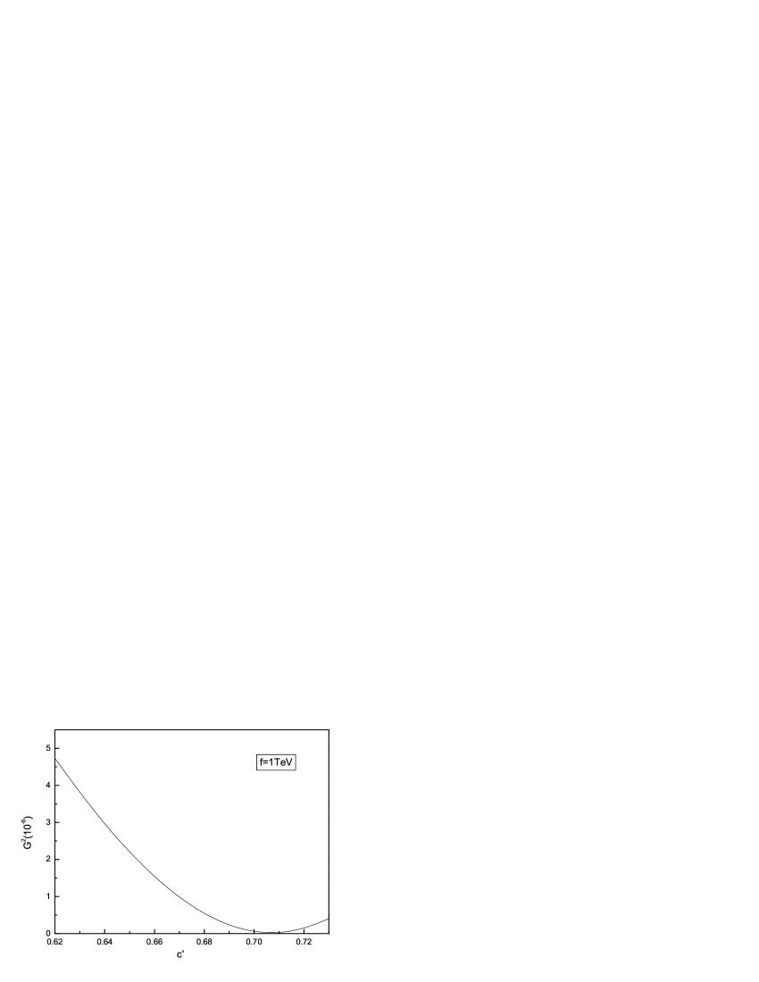
Figure 4: The plots of $G^{2}$ and $M_{B_{H}}$ as a function of $c^{\prime}$ with fixed $f=1$ TeV.

To illustrate the influence of the coupling $G$ defined in Eq.(22) and $B_{H}$ mass on the cross section, in Fig.4, we show the plots of $G^{2}$ and $M_{B_{H}}$ as a function of $c^{\prime}$ with fixed $f=1$ TeV. The change of $B_{H}$ mass $M_{B_{H}}$ can affects the phase space, but $M_{B_{H}}$ does not change very much when $c^{\prime}$ changes in the range $0.62-0.73$. So the change of the cross section mainly depends on the coupling $G$.

Since we are interested in final states where all the gauge bosons are identified, the event rate is determined not only by the total cross section, but also by the reconstruction efficiency that depends on the particular decay channels of the vector bosons. The efficiency for reconstruction of a $W^{\pm}$ is over $60\%$[17]. To identify $B_{H}$ from the final states, we also need to study its decay modes. The main decay modes of $B_{H}$ are $e^{+}e^{-}+\mu^{+}\mu^{-}+\tau^{+}\tau^{-},d\bar{d}+s\bar{s},u\bar{u}+c\bar{c},Zh,W^{+}W^{-}$. The decay branching ratios of these modes have been studied in reference [9] which are strongly dependent on the $U(1)$ charge assignments of the SM fermions. The most interesting decay modes of $B_{H}$ should be $e^{+}e^{-},\mu^{+}\mu^{-}$. This is because such particles can be easily identified and the number of $e^{+}e^{-},\mu^{+}\mu^{-}$ background events with such a high invariant mass is very small. So, a search for a peak in the invariant mass distribution of the either $e^{+}e^{-}$ or $\mu^{+}\mu^{-}$ is sensitive to the presence of $B_{H}$. In the SM, the same sufficient final states can also be produced via $\gamma\gamma\rightarrow W^{+}W^{-}Z$ with $Z\rightarrow e^{+}e^{-}(\mu^{+}\mu^{-})$, and the cross section is over $10^{2}$ fb[18]. It should be very easy to distinguish $B_{H}$ from $Z$ when we look at the invariant mass of the $e^{+}e^{-}$ or $\mu^{+}\mu^{-}$ pair because there might exist significantly different $e^{+}e^{-}$($\mu^{+}\mu^{-}$) invariant mass distribution between $B_{H}$ and $Z$. On the other hand, $B_{H}$ can also decay to $W^{+}W^{-},Zh$ and these bosonic decay modes are dominated by the longitudinal components of the final-states. In general, the decay branching ratios of $W^{+}W^{-}$ and $Zh$ are very small, but for the favorable parameter spaces we might assume enough $W^{+}W^{-}$ and $Zh$ signals to be produced with high luminosity. Such signals would provide crucial evidence that an observed new gauge boson is of the type predicted in the little Higgs models. For $B_{H}\rightarrow Zh$, the final states are $l^{+}l^{-}b\bar{b}$. Two b-jets reconstruct to the Higgs mass and a $l^{+}l^{-}$ pair reconstructs to the Z mass. On the other hand, the decay mode $Zh$ involves the off-diagonal coupling $hZB_{H}$ and the experimental precision measurement of such off-diagonal coupling is more easier than that of diagonal coupling. So, the decay mode $Zh$ would provide a better way to verify the crucial feature of quadratic divergence cancellation in Higgs mass. The decay mode $Z\rightarrow W^{+}W^{-}$ is of course kinematically forbidden in SM, but the decay $h\rightarrow W^{+}W^{-}$ is the dominant decay mode of the Higgs boson with mass above 135 GeV(one or both of the W bosons is off-shell for Higgs mass below $2M_{W}$). We leave the detailed study of such SM background to experimentalists.

The $B_{H}$ production mechanics has been studied at the LHC[10], and such particle can also be produced by $e^{+}e^{-}$ collision. However, these production processes involve the fermion couplings and these couplings suffer from large theoretical uncertainty due to the arbitrariness of the fermion $U(1)$ charge assignments. So, the reliable prediction of the $B_{H}$ signals via these processes would be difficult. On the other hand, with the small $e^{+}e^{-}B_{H}$ coupling and high energy s-channel suppression, the s-channel $B_{H}$ production in $e^{+}e^{-}$ collisions would of course be suppressed which makes $\gamma\gamma$ production mode become even more important, specially for gaining an insight into the gauge structure of the littlest Higgs model.

In summary, the new gauge bosons are the typical particles of the littlest Higgs model. With the mass in the scale of hundreds GeV, the $U(1)$ boson $B_{H}$ is the lightest one among these new gauge bosons. Therefore, such particle might provide a early signal of the littlest Higgs model at the ILC. Because the high c.m. energy can significantly enhance the cross sections of the triple gauge boson production processes, these processes become more important at the ILC.

In this paper, we study a $B_{H}$ production process associated with W boson pair via $\gamma\gamma$ collision. It can be concluded that the cross section is sensitive to the parameters $f,c^{\prime},\sqrt{s}$ which make the cross section vary from $10^{-1}$ to $10^{1}$ fb in most parameter spaces allowed by the electroweak precision data. With the favorable parameter spaces(the high c.m. energy, small $c^{\prime}$ and $f$), the sufficient events can be produced to detect $B_{H}$. On the other hand, if such gauge boson is observed at future collider experiments, the precision measurement is need which could offer the important insight for the gauge structure of the littlest Higgs model and distinguish this model from alternative theories.

Figure 1: The Feynman diagrams of the process $\gamma\gamma\rightarrow W^{+}W^{-}B_{H}$ in the littlest Higgs model.

Figure 2: The production cross section of the process $\gamma\gamma\rightarrow W^{+}W^{-}B_{H}$ as a function of the scale parameter $f$ for three different values of the mixing parameter $c^{\prime}$, with $\sqrt{s}=800$ GeV, 1500 GeV, respectively.

Figure 3: The production cross section of the process $\gamma\gamma\rightarrow W^{+}W^{-}B_{H}$ as a function of the mixing parameter $c^{\prime}$ for three different values of the scale parameter $f$ with $\sqrt{s}=1500$ GeV.

References

• [1] S. Dimopoulos and H. Georgi, Nucl. Phys. B193, 150(1981); H. P. Nilles, Phys. Rep. 110, 1(1984); H. E. Haber and G.L.Kane, ibid. 117, 75(1985); S. P. Martin, hep-ph/9709356; P. Fayet, Nucl. Phys.(Proc.Suppl.) B101, 81(2001).
• [2] For a recent review, see C. T. Hill and E. H. Simmons, Phys. Rep. 381, 235(2003).
• [3] I. Antoniadis, C. Munoz, and M. Quiros, Nucl. Phys. B397, 515(1999); N. Arkani-Hamed, S. Dimopoulos, and G. R. Dvali, Phys. Rev. D59, 086004(1999); L. Randall, R. Sundrum, Phys, Rev. Lett., 83, 4690(1999).
• [4] N. Arkani-Hamed, A. G. Cohen, and H. Georgi, Phys. Lett. B513, 232(2001).
• [5] N. Arkani-Hamed, A. G. Cohen, T. Gregoire, and J. G. Wacker, JHEP 0208 020(2002); N. Arkani-Hamed, A. G. Cohen, E. Katz, A. E. Nelson, T. Gregoire, and J. G. Wacker, JHEP 0208 021(2002).
• [6] I. Low, W. Skiba, and D. Smith, Phys. Rev. D66, 072001(2002); M. Schmaltz, Nucl. Phys. Proc. Suppl. 117, 40(2003); W. Skiba and J. Terning, Phys. Rev. D68, 075001(2003).
• [7] N. Arkani-Hamed, A. G. Cohen, E. Katz, A. E. Nelson, JHEP 0207 034(2002).
• [8] American Linear Collider Group, T. Abe etΒ al., hep-ex/0106057; ECFA/DESY LC Physics Working Group, J. A. Aguilar-Saavedra etΒ al., hep-ph/0106315; ACFA Linear Collider Working Group, K. Abe etΒ al., hep-ph/0109166.
• [9] T. Han, H. E. Logan, B. McElrath, and L. T. Wang, Phys. Rev. D67, 095004(2003).
• [10] G. Burdman, M. Perelstein, and A. Pierce, Phys. Rev. Lett. 90, 241802 (2003); T. Han, H. E. Logan, and L. T. Wang, hep-ph/0506313; G. Azuelos, K. Benslama, D. Costanzo, G. couture, J. E. Garcia, I. Hinchliffe, N. Kanaya, M. Lechowski, R. Mehdiyev, G. Polesello, E. Ros, and D. Rousseau, hep-ph/0402037; J. E. Garcia, hep-ph/0405156.
• [11] T. Abe etΒ al.[American Linear Collider Group], hep-ex/0106057; J. A. Aguilar-Saavedra etΒ al.[ECFA/DESY LC Physics Working Group], hep-ph/0106315; K. Abe etΒ al.[ACFA Linear Collider Working Group], hep-ph/0109166; G. Laow etΒ al., ILC Techinical Review Committee, second report, 2003, SLAC-R-606.
• [12] J. A. Conley, J. Hewett, and M. P. Le, Phys. Rev. D72, 115014(2005).
• [13] S. C. Park and J. Song, Phys. Rev. D69, 115010(2004); T. Han, H. E. Logen, B. McElrath, and L. T. Wang, Phys. Lett. B563, 191(2003); H. E. Logan, Phys. Rev. D70, 115003(2004); Gi-Chol cho and A. Omete, Phys. Rev. D70, 057701(2004); J. Lee, hep-ph/0408362; S. Chang and H.-J.He, Phys. Lett. B586, 95(2004); C. Csaki, J. Hubisz, G. D. Kribs, P. Meade, and J. Tering, Phys. Rev. D68, 035009(2003); C. X. Yue, W. Wei, F. Zhang, Nucl. Phys. B716, 199(2005).
• [14] G. Jikia, Nucl. Phys. B374, 83(1992); O. J. P. Eboli, etΒ al., Phys. Rev. D47, 1889(1993); K. M. Cheung, ibid. 47, 3750(1993).
• [15] J. F. Donoghue, E. Golowich, and B.R. Holstein, Dynamics of the Standard Model, Cambridge Univiversity Press, 1992, P. 34.
• [16] C. Csaki etΒ al. Phys. Rev. D68, 035009(2003); T. Gregoire, D. R. Smith, and J. G. Wacker, Phys. Rev. D69, 115008(2004); M. Chen and S. Dawson, Phys. Rev. D70, 015003(2004).
• [17] F. T. Brandt, O. J. P. Eboli, E. M. Gregores, M. B. Magro, P. G. Mercadante, and S. F. Novaes, Phys. Rev. D50, 5591(1994).
• [18] M. Baillargeon and F. Boudjema, Phys. Lett. B317, 371(1993); O. J. P. Eboli, M. B. Magro, P. G. Mercadante, and S. F. Novaes, Phys. Rev. D52, 15(1995); F. T. Brandt, O. J. P. Eboli, E. M. Gregores, M. B. Magro, P. G. Mercadante, and S. F. Novaes, Phys. Rev. D50, 5591(1994).
Refer to caption