Chemical composition of the decaying glasma

Abstract

The the initial stage of a relativistic heavy ion collision can be described by a classical color field configuration known as the Glasma. The production of quark pairs from this background field is then computed nonperturbatively by numerically solving the Dirac equation in the classical background. The result seems to point towards an early chemical equilibration of the plasma.

1 Introduction

At large energies (small $x$) the hadron/nucleus wavefunction is characterized by a saturation scale $Q_{\mathrm{s}}$ arising from the strong nonlinear interactions between the wee partons, mostly gluons. If the energy is high enough so that $Q_{\mathrm{s}}\gg\Lambda_{\mathrm{QCD}}$, weak coupling methods can be used to decribe physics at transverse momenta $\sim Q_{\mathrm{s}}$. In the context of ultrarelativistic heavy ion collisions this means that one can hope to understand not only hard probes, but the bulk of particle production in terms of weak coupling, deconfined physics. Note that although the coupling is weak, the saturated color fields are strong $A_{\mu}\sim 1/g$, and the physics must still be treated nonperturbatively.

The purpose of this talk is to explore the initial state of a heavy ion collision in this framework. We will first describe what has been called the Glasma [1], a highly coherent classical field in the initial stage of the collision. We will then move on to study how quark pairs can be produced from this, to a first approximation, purely gluonic system, moving it closer to a chemically equilibrated plasma of both quarks and gluons [2, 3].

2 Glass and Glasma

The small $x$ wavefunction of a hadron or nucleus, characterized by nonperturbatively large color fields, can be described in terms of a classical Weizsäcker-Williams (WW) field radiated by the hard, large $x$, sources. Because of their high speed and Lorentz time dilation, the hard degrees of freedom are seen by the low $x$ fields as slowly evolving in lightcone time. They can therefore be thought of as classical, static (in light cone time) sources for the small $x$ fields [4]. This effective description has been called the Color Glass Condensate. The earliest stage of an ultrarelativistic heavy ion collision is a coherent, classical field configuration of two colliding sheets of Color Glass. This first fraction of a fermi of the collision, in transition from two sheets of Color Glass into eventually a quark gluon plasma, is what we refer to as the Glasma [1].

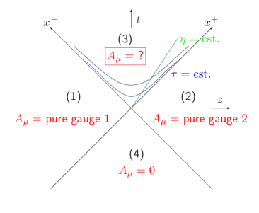
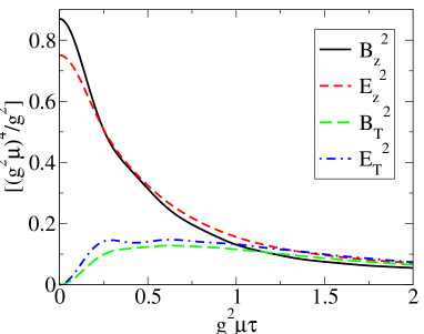
Figure 1: Left: The $A_{\tau}=0$-gauge field in different regions of spacetime. Right: Components of the glasma field as a function of $g^{2}\mu\tau$ in units of $(g^{2}\mu)^{4}/g^{2}$

The color fields of the two nuclei are transverse electric and magnetic fields on the light cone. The glasma fields left over in the region between the two nuclei after the collision at times $1\leq\tau\leq 1/Q_{\mathrm{s}}$ are, however, longitudinal along the beam axis. One way of understanding these field configurations is the following. Let us work in light cone gauge, so that each nucleus, when going past a point on the beam axis with no gauge field before the collision, leaves behind it a pure gauge field (see Fig. 1). One can define an effective chromoelectric and chromomagnetic charge density by separating the nonlinear parts of the vacuum Gauss law and Bianchi identities

$$\left[D_{i},E^{i}\right]=0\quad\textrm{ and }\quad\left[D_{i},B^{i}\right]=0$$ (1)

as

$$\partial_{i}E^{i}=\rho_{\mathrm{e}}=ig[A^{i},E^{i}]\quad\textrm{ and }\quad\partial_{i}B^{i}=\rho_{\mathrm{m}}=ig[A^{i},B^{i}].$$ (2)

Now we can interpret the interaction of the WW chromoelectric and -magnetic fields of the nucleus on the $x^{+}$-light cone with the pure gauge field left behind by the other nucleus as an effective chromoelectric and -magnetic charge density left behind on the light cone. An exactly opposite charge density is left behind on the other sheet, leading to a longitudinal chromoelectric and -magnetic field between the sheets . This structure is illustrated in Fig. 2.

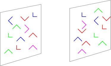
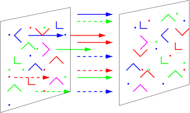
Figure 2: The WW fields of the two nuclei before and after the collision. Before the collision there are only transverse fields on the sheets. After the collision the interaction of these fields with the pure gauge field of the other nucleus leaves behind an effective electric and magnetic charge density (the dots on the figure) on the sheet, and a longitudinal electric and magnetic field between these effective charges.

As the initial condition has a chromoelectric and -magnetic field both in the longitudinal direction, it also has a nonzero Chern-Simons charge density $\sim g^{2}\epsilon^{\mu\nu\rho\sigma}\tr F_{\mu\nu}F_{\rho\sigma}$, fluctuating on transverse length scales of the inverse saturation momentum. This can naturally lead to large P- and CP-violations in these domains, which could have interesting consequences as parity-odd global observables in the produced mesons [5, 6, 7, 8]. If the gauge field configurations are exactly boost invariant, no topologically nontrivial configurations (sphaleron transitions) are allowed [9], and the effect is suppressed. But as giving up the assumption of boost invariance in the numerical calculation is becoming more feasible [10, 11] one will be able to understand this phenomenon better.

How, then, does the glasma decay into plasma, i.e. how can we move from a description of the initial state in terms of classical fields into one formulated for quantum particles? The glasma fields depend on the transverse coordinate on a length scale of order $1/Q_{\mathrm{s}}$. Thus to lowest order (in the coupling $\alpha_{\mathrm{s}}$ or in $\hbar$) the fields simply radiate away as gluons with ${\mathbf{p}_{T}}\sim Q_{\mathrm{s}}$. As the system expands the fields are diluted and can be treated as particles. This lowest order production is the contribution that is computed in the numerical computations of gluon production in heavy ion collisions [12, 13, 14, 15, 16].

In the rest of this paper we will be concerned with the next order in $g$ or $\hbar$, namely quantum pair production from the classical background field. Both gluons and quarks carry color charge and can be produced in pairs from the background field. The production of gluon pairs is the first quantum correction to the classical background field. To consistently compute it one must take care to avoid double counting the gluons that are already effectively included in the classical background field. A calculation of gluon pair production must be done consistently with the high energy renormalization group evolution of the sources. This computation has not yet been precisely formulated. On the other hand, computing quark pair production from the classical background field is more directly relevant for the phenomenology of heavy ion collisions and easier to formulate, if not necessarily trivial to carry out nonperturbatively, because it only involves the lowest order classical gluon field.

3 Background field from the MV model

The hard degrees of freedom are modeled as classical sources on the light cones:

$$J^{\mu}=\delta^{\mu+}\rho_{(1)}(\mathbf{x}_{T})\delta(x^{-})+\delta^{\mu-}\rho_{(2)}(\mathbf{x}_{T})\delta(x^{+}).$$ (3)

The Weizsäcker-Williams fields describing the softer degrees of freedom can then be computed from the classical Yang-Mills equation $[D_{\mu},F^{\mu\nu}]=J^{\nu}$. In the light cone gauge the field of one nucleus is a pure gauge outside the light cone (see Fig. 1)

$$A^{i}_{(1,2)}=\frac{i}{g}U_{(1,2)}\partial_{i}U^{\dagger}_{(1,2)},\textrm{ with }U_{(m)}(\mathbf{x}_{T})=\exp\left\{-ig\frac{\rho_{(m)}(\mathbf{x}_{T})}{{\boldsymbol{\nabla}_{T}}^{2}}\right\}.$$ (4)

In the original MV model, which we shall be using here, the color charge densities are stochastic Gaussian random variables on the transverse plane

$$\langle\rho^{a}(\mathbf{x}_{T})\rho^{b}(\mathbf{y}_{T})\rangle=g^{2}\mu^{2}\delta^{ab}\delta^{2}(\mathbf{x}_{T}-\mathbf{y}_{T}),$$ (5)

where the density of color charges $g^{2}\mu$ is, up to a numerical constant and a logarithmic uncertainty, proportional to the saturation scale $Q_{\mathrm{s}}$.

The initial conditions for the fields in the future light cone between the two colliding sheets were derived and the equations of motion solved to lowest order in the fields in Refs. [17, 18] (see also Ref. [19] for the same calculation in covariant gauge and Ref. [20] for another formulation of the same lowest order result.) This initial condition has a simple expression in terms of the pure gauge fields (4) of the two colliding nuclei:

$$A^{i}=A^{i}_{(1)}+A^{i}_{(1)}\quad\textrm{ and }\quad A^{\eta}=\frac{ig}{2}\left[A^{i}_{(1)},A^{i}_{(2)}\right].$$ (6)

The solution of the Yang Mills equations beyond leading order is not known analytically. They can, however, be solved numerically on the lattice. The numerical setup was formulated in Ref. [12] and used to calculate the energy density and gluon multiplicity corresponding to the glasma fields in e.g. Refs. [12, 13, 14, 15, 16]. It is these numerically computed color field configurations that we will use as the background field for computing quark production in the following.

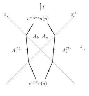
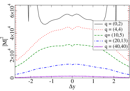
Figure 3: Left: Spacetime in Dirac equation. In the case when the nuclei move exactly at the speed of light the solution decomposes into two distinct paths depending on whether the $x^{+}$ or $x^{-}$ light cone is encoutered first. In the Abelian case these correspond to the $t$ and $u$ channel terms of the amplitude. Right: amplitude as a function of rapidity $y_{p}-y_{q}$ for different transverse momentum modes ${\mathbf{q}_{T}}$.

4 Pair production

Let us then move on to the computation of quark pair production from the background color field described above starting with a few trivial remarks:

• We are assuming such a high collision energy that the nuclear wavefunction is completely gluonic and the process $gg\to q\bar{q}$ dominates over quark production from the sea and valence distributions by processes like $qg\to qg$. This might not yet be a very good approximation at RHIC energies [21]. We are also neglecting the backreaction of the produced pairs on the gluon fields.

• When the computation of gluon production to the lowest order is done nonperturbatively to all orders in the strong field the multiplicity and energy density of the gluons is infrared finite. But for the computation of quark pair production it is not a priori evident whether the limit $m_{q}\to 0$ is finite.

• If quark production is dominated by saturation physics, one could expect production to be flavor blind for $m_{q}\ll Q_{\mathrm{s}}$. Thus strangeness would, from the beginning, be equilibrated with the light flavors.

Our method of computing quark pair production by solving the Dirac equation is explained in more detail in Ref. [2]. One starts, at $t\to-\infty$ with a negative energy plane wave solution of the free Dirac equation, $e^{iq\cdot x}v(q)$ (see Fig. 3). The Dirac equation is solved forward in time until $t\to\infty$, and the solution projected on positive energy plane wave states $e^{-ip\cdot x}u(p)$. The amplitude is then interpreted as the amplitude to produce a quark pair from the classical background field. Solving the Dirac equation forward in time is equivalent to computing the full retarded (not Feynman) Dirac propagator in the background field. This means [22] that one is computing the expectation value of the number of pairs produced, not the cross section to produce exactly one pair (which would be related to the Feynman propagator). The formal derivation of this procedure is given in Ref. [22], but the physical interpretation is perhaps more intuitive in terms of the “Dirac sea”. Picturing the vacuum as a Dirac sea with all the negative energy states filled, one is taking a component of the “in” vacuum (at $t\to-\infty$) and computing its overlap with an “out” state (at $t\to\infty$) of a quark with momentum $p$. If this overlap is nonzero, the background field has lifted a negative energy solution from the Dirac sea to positive energy, leaving a hole in the sea. This process is then interpreted as the creation of a pair of fermions.

Because the background field of one nucleus is a pure gauge (see Figs. 1 and 3), the Dirac equation can be solved analytically up to the future light cone ($x^{+}=0$, $x^{-}>0$ and $x^{-}=0$, $x^{+}>0$). In the Abelian case also the field inside the future light cone is a pure gauge, and the whole computation (electron positron pairs in ultraperipheral collisions of two heavy ions) can be carried through analytically [23]. In our case the field inside the future light cone is only known numerically, and so we must solve the Dirac equation numerically starting from an analytically derived initial condition at $\tau=0$. It turns out that this is most conveniently done in the $(\tau,z,\mathbf{x}_{T})$–coordinate system. The natural choice for the temporal coordinate is $\tau$, because the initial condition for the numerical computation is given at $\tau=0$, and thus no other time coordinate would lead to a pure initial value problem. For the longitudinal coordinate one must (unlike the three dimensional computation of the color field in Refs. [10, 11]) choose a dimensional coordinate in order to represent the longitudinal momenta ($q^{\pm}$) on a coordinate space lattice at $\tau=0$.

It was shown in Ref. [24] that in the lowest this calculation of pair production reduces to a standard expression in ${\mathbf{k}_{T}}$–factorized perturbation theory. The “pA” case, when only one of the classical color fields is treated to lowest order, can also be solved analytically [25]. A ${\mathbf{k}_{T}}$–factorized perturbative formalism has also been used to compute production of heavy quarks in from the “Color Glass Condensate” gluon distributions e.g. in Ref. [26]. A way of approaching the problem from the other limit is presented in Ref. [27], where, using the WKB approximation, pair production is computed nonperturbatively in a short longitudinal color field pulse, neglecting the magnetic field. Because this computation also neglects the transverse coordinate dependence of the field, it cannot reduce to the same perturbative expression in the weak field limit.

Let us then finally move to the results of the numerical computation [3]. The computation has three independent numerical parameters, the color charge density $g^{2}\mu$ that determines the strength of the background field, the nuclear radius $R_{A}$ giving the size of the system in the transverse plane, and $m$, the quark mass. Figure 3 shows the amplitude, integrated over the momentum of the quark but for different transverse momenta of the antiquark, as a function of the rapidity difference $\Delta y\equiv y_{p}-y_{q}$ between the quark and the antiquark. Because the background field is boost invariant, this amplitude only depends on $\Delta y$ and not the rapidity of the whole system $(y_{p}+y_{q})/2$. When also integrating over $\Delta y$ one gets the spectrum as a function of the transverse momentum of the antiquark, shown in Fig. 4 for different strengths of the background color fields. On a finite lattice the large ${\mathbf{p}_{T}}$ part of the spectrum is affected by the proximity of the lattice cutoff $\sim 1/a$, which is demonstrated in Fig. 5, where the same spectrum is plotted for different values of the lattice cutoff. Although physically the quarks can only be interpreted as on shell particles after a formation time $\sim 1/m_{\mathrm{T}}$, the projection on positive energy estates can be done at arbitrarily early times. A shown in Fig. 5 the amplitude is close to its final value for very early times close to the light cone.

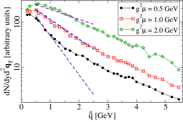
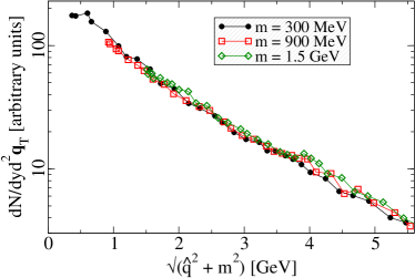
Figure 4: Left: Antiquark transverse momentum spectrum for different values of the classical color charge density $g^{2}\mu$ for $m=0.3\textrm{ GeV}$. The straight lines to (mis)guide the eye are $\sim e^{-{\mathbf{q}_{T}}/(g^{2}\mu)}$. Right: The antiquark spectrum as a function of the transverse mass $\sqrt{{\mathbf{q}_{T}}^{2}+m^{2}}$ for different masses and $g^{2}\mu=1\textrm{ GeV}$.

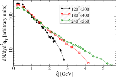
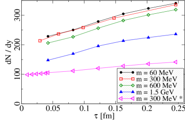
Figure 5: Left: Amplitude with $m=0.3\textrm{ GeV}$ and $g^{2}\mu=1\textrm{ GeV}$ for different lattice sizes, corresponding to different values of the ultraviolet lattice cutoff. Right: Amplitude as a function of the time at which the projection to positive energy states is done. The first four data sets are for $g^{2}\mu=2\textrm{ GeV}$ and the last one (marked with an asterisk) for $g^{2}\mu=1\textrm{ GeV}$.

According to conventional wisdom the initial state of a heavy ion collision is dominated by gluons. Assuming that the subsequent evolution of the system conserves entropy this would mean $\sim 1000$ gluons in a unit of rapidity. In the classical field model this corresponds [16] to $g^{2}\mu=2\textrm{ GeV}$. Our result seems to point to a rather large number of quark pairs present already in the initial state. One could envisage a scenario where, for $g^{2}\mu=1.3\textrm{ GeV}$, these 1000 particles could consist of 400 gluons, 300 quarks and 300 antiquarks (take the lowest curve from Fig. 5 and mutiply by $N_{\mathrm{f}}=3$). This would be close to the thermal ratio of $N_{q}/N_{g}=9N_{\mathrm{f}}/32$.

5 Conclusions

We have pointed out some known, but not always fully appreciated, features of the classical field description of the early stages of a heavy ion collision. The “Glasma” fields are initially longitudinal chromoelectric and chromomagnetic fields, of equal magnitude. These fields can be thought of as arising from effective chromoelecric and -magnetic charge densities on the transverse planes caused by the color rotation of the Weizsäcker-Williams fields of one nucleus in the pure gauge field of the other.

We have then studied quark pair production from classical background field of McLerran-Venugopalan model studied by solving the 3+1–dimensional Dirac equation numerically in this classical background field. We find that the number of quarks produced large, potentially leading to a very early chemical equilibration of the quark and gluon degrees of freedom. But in order to put this conclusion on a more theoretically sound footing one must also compute gluon production to the same order in the couopling $\alpha_{\mathrm{s}}$, which has not yet been done. Our numerical method does not yet allow us to extend our method to large quark masses or transverse momenta.

References

References

- [1] T. Lappi and L. McLerran, Nucl. Phys. A772 (2006) 200 [hep-ph/0602189].
- [2] F. Gelis, K. Kajantie and T. Lappi, Phys. Rev. C71 (2005) 024904 [hep-ph/0409058].
- [3] F. Gelis, K. Kajantie and T. Lappi, Phys. Rev. Lett. 96 (2006) 032304 [hep-ph/0508229].
- [4] L. D. McLerran and R. Venugopalan, Phys. Rev. D49 (1994) 2233 [hep-ph/9309289].
- [5] D. Kharzeev, R. D. Pisarski and M. H. G. Tytgat, Phys. Rev. Lett. 81 (1998) 512 [hep-ph/9804221].
- [6] D. Kharzeev and R. D. Pisarski, Phys. Rev. D61 (2000) 111901 [hep-ph/9906401].
- [7] D. Kharzeev, Phys. Lett. B633 (2006) 260 [hep-ph/0406125].
- [8] STAR Collaboration, I. V. Selyuzhenkov, nucl-ex/0510069.
- [9] D. Kharzeev, A. Krasnitz and R. Venugopalan, Phys. Lett. B545 (2002) 298 [hep-ph/0109253].
- [10] P. Romatschke and R. Venugopalan, Phys. Rev. Lett. 92 (2006) 062302 [hep-ph/0510121].
- [11] P. Romatschke and R. Venugopalan, hep-ph/0605045.
- [12] A. Krasnitz and R. Venugopalan, Nucl. Phys. B557 (1999) 237 [hep-ph/9809433].
- [13] A. Krasnitz and R. Venugopalan, Phys. Rev. Lett. 84 (2000) 4309 [hep-ph/9909203].
- [14] A. Krasnitz and R. Venugopalan, Phys. Rev. Lett. 86 (2001) 1717 [hep-ph/0007108].
- [15] A. Krasnitz, Y. Nara and R. Venugopalan, Phys. Rev. Lett. 87 (2001) 192302 [hep-ph/0108092].
- [16] T. Lappi, Phys. Rev. C67 (2003) 054903 [hep-ph/0303076].
- [17] A. Kovner, L. D. McLerran and H. Weigert, Phys. Rev. D52 (1995) 3809 [hep-ph/9505320].
- [18] M. Gyulassy and L. D. McLerran, Phys. Rev. C56 (1997) 2219 [nucl-th/9704034].
- [19] Y. V. Kovchegov and D. H. Rischke, Phys. Rev. C56 (1997) 1084 [hep-ph/9704201].
- [20] R. J. Fries, J. I. Kapusta and Y. Li, nucl-th/0604054.
- [21] K. J. Eskola and K. Kajantie, Z. Phys. C75 (1997) 515 [nucl-th/9610015].
- [22] A. J. Baltz, F. Gelis, L. D. McLerran and A. Peshier, Nucl. Phys. A695 (2001) 395 [nucl-th/0101024].
- [23] A. J. Baltz and L. D. McLerran, Phys. Rev. C58 (1998) 1679 [nucl-th/9804042].
- [24] F. Gelis and R. Venugopalan, Phys. Rev. D69 (2004) 014019 [hep-ph/0310090].
- [25] H. Fujii, F. Gelis and R. Venugopalan, Phys. Rev. Lett. 95 (2005) 162002 [hep-ph/0504047].
- [26] D. Kharzeev and K. Tuchin, Nucl. Phys. A735 (2004) 248 [hep-ph/0310358].
- [27] D. Kharzeev, E. Levin and K. Tuchin, hep-ph/0602063.