DEPUZZLING $B\rightarrow K\pi$ : CONSTRAINTS ON THE UNITARITY TRIANGLE FROM $B,B_{s}\rightarrow\pi\pi,K\pi,KK$ DECAYS IN THE $SU(3)$ LIMIT

Constraining CKM parameters from charmless hadronic $B$ decays requires methods for addressing the hadronic uncertainties. A complete technique is presented, using relations between amplitudes in the $B,B_{s}\rightarrow\pi\pi,K\pi,KK$ system obtained in the exact $SU(3)$ symmetry limit, without having to neglect annihilation/exchange topologies. Naive $SU(3)$-breaking effects in the decay amplitudes are taken into account, through the inclusion of $\pi$ and $K$ decay constants in the normalisations and conservative theoretical errors. Already with the limited set of observables currently available, significant constraints on the CKM parameters are obtained. Also, subsets of observables are shown to bring non trivial constraints on the CKM angles $\alpha$ and $\beta$, in agreement with analytical solutions that we derive. Finally, the future physics potential of this method is estimated, in light of the increased precision of measurements from the current B-factories, and the inclusion of several new observables from $B_{s}$ decays expected to be provided by the LHC experiments.

1 Introduction

Constraining CKM parameters from charmless hadronic $B$ decays requires methods for addressing the hadronic uncertainties. A common method consists in considering symmetries to relate different decay amplitudes and eliminate hadronic unknowns. SU(2) symmetry is well understood and largely used to get constraints on the Unitarity Triangle from charmless two-body hadronic $B$ decays. In the $\pi\pi$ system, it allows to determine the angle $\alpha$ up to an eightfold ambiguity, whereas in the $K\pi$ system, it requires additional hypotheses to be predictive. In both cases, the derived constraints remain weak with the current errors and one can wonder how to use all the available inputs in a more efficient manner. Although errors remain large, theoretical calculations as SCET or QCD factorization can be considered, as it has been discussed previously $\!{}^{{\bf?},{\bf?}}$. Here, we propose a new data-driven technique, using relations between amplitudes in the $B,B_{s}\rightarrow\pi\pi,K\pi,KK$ system obtained in the $SU(3)$ symmetry limit. Use of approximate SU(3) symmetry $\!{}^{{\bf?}}$ for those modes has received considerable attention in the recent literature $\!{}^{{\bf?},{\bf?},{\bf?},{\bf?}}$. In this paper, the exact $SU(3)$ limit is considered, without additional hypotheses such as the neglect of annihilation/exchange topologies. Naive $SU(3)$-breaking effects in the decay amplitudes are taken into account, through the inclusion of $\pi$ and $K$ decay constants in the normalisations and conservative theoretical errors.

The first section is devoted to the formalism: the decay amplitudes under $SU(3)$ are expressed, electroweak penguin amplitudes are related to other amplitudes in a model-independent way, and the SU(3) breaking parameterization is described. In section 3, two analytically solvable subsystems of observables are introduced mainly constraining the CKM angles $\alpha$ and $\beta$. The inputs, the parameter counting and the statistical approch are briefly discussed in section 4. Finally, numerical results are given in section 5, where the future physics potential of this method is also estimated, in light of the increased precision of measurements from the current B-factories, and the inclusion of several new observables from $B_{s}$ decays expected to be provided by the LHC experiments. This work will be described in further details in an upcoming publication $\!{}^{{\bf?}}$.

2 Formalism

2.1 Model-independent parameterization in the SU(3) limit

Benefiting from the unitarity of the CKM matrix, one can provide a phenomenological description of any decay amplitude in terms of CKM matrix elements and two complex hadronic amplitudes; namely for the $B^{0}\rightarrow K^{+}\pi^{-}$ decay amplitude: $A(K^{+}\pi^{-})=V_{us}V_{ub}^{*}\,T^{+-}+V_{ts}V_{tb}^{*}\,P$. Owing to SU(3) invariance of strong interaction, the amplitudes of various $B,B_{s}\rightarrow\pi\pi,K\pi,KK$ decays are related to each other through 16 complex independent equations, and thus the system can be described via only 10 hadronic amplitudes, i.e. 19 real physical parameters, as follows:

$$A(B_{d}\rightarrow K^{+}\pi^{-}) = V_{us}V_{ub}^{*}\,T^{+-}+V_{ts}V_{tb}^{*}\,P\leavevmode\nobreak\ ,$$

$$A(B_{u}\rightarrow K^{0}\pi^{+}) = V_{us}V_{ub}^{*}\,N^{0+}+V_{ts}V_{tb}^{*}\,(-P+P^{EW}_{C}),$$

$$A(B_{u}\rightarrow K^{+}\pi^{0}) = V_{us}V_{ub}^{*}\,(T^{+-}+T^{00}-N^{0+})+V_{ts}V_{tb}^{*}\,(P+P^{EW}-P^{EW}_{C})\leavevmode\nobreak\ ,$$

$$A(B_{d}\rightarrow K^{0}\pi^{0}) = V_{us}V_{ub}^{*}\,T^{00}+V_{ts}V_{tb}^{*}\,(-P+P^{EW})\leavevmode\nobreak\ ,$$

$$A(B_{d}\rightarrow\pi^{+}\pi^{-}) = V_{ud}V_{ub}^{*}\,(T^{+-}+\Delta T)+V_{td}V_{tb}^{*}\,(P+PA)\leavevmode\nobreak\ ,$$

$$A(B_{d}\rightarrow\pi^{0}\pi^{0}) = V_{ud}V_{ub}^{*}\,(T^{00}-\Delta T)+V_{td}V_{tb}^{*}\,(-P-PA+P^{EW})\leavevmode\nobreak\ ,$$

$$A(B_{u}\rightarrow\pi^{+}\pi^{0}) = V_{ud}V_{ub}^{*}\,(T^{+-}+T^{00})+V_{td}V_{tb}^{*}\,P^{EW}\leavevmode\nobreak\ ,$$

$$A(B_{d}\rightarrow K^{+}K^{-}) = V_{ud}V_{ub}^{*}\,\Delta T+V_{td}V_{tb}^{*}\,PA\leavevmode\nobreak\ ,$$

$$A(B_{d}\rightarrow K^{0}\bar{K^{0}}) = V_{ud}V_{ub}^{*}\,\Delta P+V_{td}V_{tb}^{*}\,(-P-PA+P^{EW}_{C}-\frac{1}{2}P^{EW}_{K\bar{K}})\leavevmode\nobreak\ ,$$

$$A(B_{u}\rightarrow K^{+}\bar{K^{0}}) = V_{ud}V_{ub}^{*}\,N^{0+}+V_{td}V_{tb}^{*}\,(-P+P^{EW}_{C})\leavevmode\nobreak\ ,$$

$$A(B_{s}\rightarrow K^{+}K^{-}) = V_{us}V_{ub}^{*}\,(T^{+-}+\Delta T)+V_{ts}V_{tb}^{*}\,(P+PA)\leavevmode\nobreak\ ,$$

$$A(B_{s}\rightarrow K^{+}\pi^{-}) = V_{ud}V_{ub}^{*}\,T^{+-}+V_{td}V_{tb}^{*}\,P\leavevmode\nobreak\ ,$$

$$A(B_{s}\rightarrow\pi^{+}\pi^{-}) = V_{us}V_{ub}^{*}\,\Delta T+V_{ts}V_{tb}^{*}\,PA\leavevmode\nobreak\ .$$ (1)

These equations are perfectly exact in the SU(3) limit.

2.2 Electroweak penguins from $Q_{9,10}$ dominance

One can relate the electroweak penguins amplitudes $P^{\mathrm{EW}}$, $P^{\mathrm{EW}}_{\mathrm{C}}$ and $P^{EW}_{K\bar{K}}$ to the other amplitudes in a model-independent way $\!{}^{{\bf?},{\bf?}}$ in the SU(3) limit making use of Fierz transforms and benefiting from the dominance of the operator $c_{9}O_{9}+c_{10}O_{10}$ with respect to $c_{7}O_{7}+c_{8}O_{8}$:

$$P^{\mathrm{EW}} = R^{+}\left(T^{+-}+T^{00}\right)\leavevmode\nobreak\ ,$$

$$P^{\mathrm{EW}}_{\mathrm{C}} = \frac{R^{+}}{2}\left(T^{+-}+T^{00}+N^{0+}-\Delta T-\Delta P\right)-\frac{R^{-}}{2}\left(T^{+-}-T^{00}+N^{0+}+\Delta T+\Delta P\right)\leavevmode\nobreak\ ,$$

$$P^{\mathrm{EW}}_{\mathrm{K\bar{K}}} = \frac{R^{+}}{2}\left(N^{0+}-\Delta T-\Delta P\right)\leavevmode\nobreak\ .$$ (2)

In the above equations $R^{+}$ and $R^{-}$ are constants given by

$$R^{+}=-\frac{3}{2}\frac{c_{9}+c_{10}}{c_{1}+c_{2}}\;=\;+(1.35\pm 0.12)\leavevmode\nobreak\ 10^{-2}\leavevmode\nobreak\ ,\leavevmode\nobreak\ \leavevmode\nobreak\ R^{-}=-\frac{3}{2}\frac{c_{9}-c_{10}}{c_{1}-c_{2}}\;=\;+(1.35\pm 0.13)\leavevmode\nobreak\ 10^{-2}\leavevmode\nobreak\ .$$ (3)

The theoretical error on the numerical evaluation of this ratio has been estimated from the residual scale and scheme dependence of the Wilson coefficients $\!{}^{{\bf?}}$.

2.3 SU(3) breaking

SU(3) flavor symmetry is only approximately realized in nature and one may expect violations up to $30\%$ at the amplitude level. For example, within factorization the relative size of SU(3) symmetry breaking is expected to be $(f_{K}-f_{\pi})/f_{K}$, where $f_{K}$ and $f_{\pi}$ are the pion and kaon decay constants, respectively. Dominant factorizable SU(3) breaking effects $\!{}^{{\bf?}}$ are taken into account via the normalization of $B\rightarrow K\pi$, $B\rightarrow K\bar{K}$ and $B_{s}\rightarrow K\pi$ amplitudes, with regard to the $B\rightarrow\pi\pi$ one. The normalization factors are respectively:

$$N_{K\pi} = \frac{f_{K}}{f_{\pi}}=1.22\pm 0.22\leavevmode\nobreak\ ,$$

$$N_{K\bar{K}} = \left(\frac{f_{K}}{f_{\pi}}\right)^{2}\frac{f_{B_{s}}}{f_{B_{d}}}=1.81\pm 0.34\leavevmode\nobreak\ ,$$

$$N^{s}_{K\pi} = \frac{f_{K}}{f_{\pi}}\frac{f_{B_{s}}}{f_{B_{d}}}=1.48\pm 0.28\leavevmode\nobreak\ ,$$ (4)

where the theoretical uncertainty of $22\%$ is calculated taking the error on $\frac{f_{K}}{f_{\pi}}$ to be its deviation from one. Remaining SU(3) breaking effects are neglected: residual factorizable SU(3) breaking does not exceed a few percents, while non factorizable SU(3) breaking sources, being unconstrained by both theoretical and experimental arguments for the moment, are assumed to play no important role.

3 Some observables subsets

Within this framework, one can first reduce the number of unknowns by considering subsystems of observables constraining the angles $\alpha$ and $\beta$ separately. These subsystems are of great interest because they dominate the constraints in the ($\overline{\rho}$,$\overline{\eta}$) plane and they can be solved analytically. For the sake of simplicity, we will give the analytical solutions in the case of vanishing annihilation and exchange topologies. Note that analytical solutions do still exist without this hypothesis, and that the numerical results do not neglect these contributions.

3.1 The “$\alpha$” subsystem

Let us first consider all the observables related to $B^{0}\rightarrow\pi^{+}\pi^{-}$, $B^{0}\rightarrow K^{+}\pi^{-}$, and $B^{0}\rightarrow K^{+}K^{-}$ decays and call this subsystem “$\alpha$”. In this case, the system reduces to 4 complex hadronic unknowns: $T^{+-}$, $P$, $\Delta T$ and $PA$. Neglecting annihilation and exchange topologies ($\Delta T=PA=0$), the system can be described by two equations, in the $V_{us}V_{ub}^{*},V_{cs}V_{cb}^{*}$ basis:

$$A(B\rightarrow K^{+}\pi^{-})=te^{i\gamma}-p\leavevmode\nobreak\ ,A(B\rightarrow\pi^{+}\pi^{-})=\lambda te^{i\gamma}-\frac{1}{\lambda}p\leavevmode\nobreak\ ,\\$$

solving to the analytical solution:

$$\sqrt{1-C_{\pi\pi}^{+-\,2}}|\mathcal{D}|\cos(2\alpha-2\alpha_{\mathrm{eff}}-\epsilon)=(1+\lambda^{2})^{2}-2\lambda^{2}sin^{2}(\gamma)\left(1+\frac{{\cal B}_{K\pi}^{+-}}{{\cal B}_{\pi\pi}^{+-}}\right)\leavevmode\nobreak\ ,$$ (5)

with ${\cal B}_{K\pi}^{+-}C_{K\pi}^{+-}+{\cal B}_{\pi\pi}^{+-}C_{\pi\pi}^{+-}=0$ and $\mathcal{D}\equiv|\mathcal{D}|e^{i\epsilon}=(1+\lambda^{2})\,(1+\lambda^{2}e^{i\gamma})$. Thus, this subsystem mainly measures the angle $\alpha$, with a $\lambda^{2}$ suppressed dependence on the angle $\gamma$ ($\lambda=\sin(\theta_{\rm Cabibbo})\sim 0.23$).

3.2 The “$\beta$” subsystem

Let us now consider the subsystem of observables related to $B^{0}\rightarrow\pi^{0}\pi^{0}$, $B^{0}\rightarrow K^{0}\pi^{0}$, and $B^{0}\rightarrow K^{+}K^{-}$ decays. In the same manner than for the “$\alpha$” subsystem, the hadronic unknowns are reduced to four complex quantities $T^{00}$, $-P+P^{EW}$, $\Delta T$ et $PA$. Neglecting annihilation and exchange topologies, it solves to:

$$\sqrt{1-C_{K\pi}^{00\,2}}|\mathcal{D}|\cos(2\beta-2\beta_{\mathrm{eff}}+\epsilon)=(1+\lambda^{2})^{2}-2\lambda^{2}sin^{2}(\gamma)\left(1+\frac{{\cal B}_{\pi\pi}^{00}}{{\cal B}_{K\pi}^{00}}\right)\leavevmode\nobreak\ ,$$ (6)

with ${\cal B}_{K\pi}^{00}C_{K\pi}^{00}+{\cal B}_{\pi\pi}^{00}C_{\pi\pi}^{00}=0$. This subsystem, called “$\beta$” in the following, mainly measures the angle $\beta$, with a $\lambda^{2}$ suppressed dependence on the angle $\gamma$.

4 Input data, parameter counting and statistical approach

The inputs used are world averages from HFAG $\!{}^{{\bf?}}$ at EPS 2005, using available results from BABAR, Belle, CLEO and CDF. We have used ten branching ratios, eight CP asymmetries, and the two CP parameters $S^{+-}_{\pi\pi}$ and $S^{00}_{K_{S}\pi}$; i.e. 20 independent observables in total for the $B_{d}$ and $B_{u}$ amplitudes. In addition, we have taken into account six ratios of branching ratios measured by CDF, four of which are the only observables available for $B_{s}$ decays.

For the “$\alpha$” and “$\beta$” subsystems, we have respectively 8 and 6 measurements available, both corresponding to 6 independent observables, for a total of 7 real hadronic unknowns for each system. For the full system, we already have in total 21 independent observables for 13 real hadronic unknowns. There are up to 38 independent observables related to this system making it a promising tool to constraint the Unitarity Triangle in the future.

We use classical frequentist statistics (minimum $\chi^{2}$) to obtain the constraints on the parameters. All unknown parameters are left free to vary in the fit without contributing to the $\chi^{2}$. As for the parameters that come with a theoretical uncertainty (namely $R^{\pm}$, and the normalization factors in (4)), we use the Rfit $\!{}^{{\bf?}}$ approach.

5 Fit results

5.1 The “$\alpha$” and “$\beta$” subsystems

Constraints in the ($\overline{\rho}$,$\overline{\eta}$) plane for the “$\alpha$” and “$\beta$” subsystems are shown on figure 1. The respective dependence on the angles $\alpha$ and $\beta$ is clearly visible, whereas the dependences on the angle $\gamma$ create small structures breaking the symmetry of the constraints. Both results are in good agreement with the superimposed standard CKM fit.

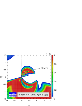
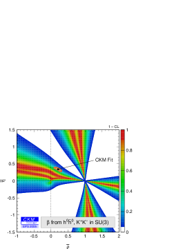
Figure 1: Constraints in the ($\overline{\rho}$,$\overline{\eta}$) plane from $B\rightarrow\pi^{+}\pi^{-},K^{+}\pi^{-},K^{+}K^{-}$ modes, i.e. from the “$\alpha$” subsystem of inputs (left) and from $B\rightarrow\pi^{0}\pi^{0},K^{0}\pi^{0},K^{+}K^{-}$ modes, i.e. from the “$\beta$” subsystem of inputs (right).

5.2 Joint and full systems

Correlations between the two subsystems arise from two sources: the common mode $B_{d}\rightarrow K^{+}K^{-}$ and the tree-dependent parameterization of the electroweak penguins amplitude $P^{EW}$. If $P^{EW}$ was totally free, $-P+P^{EW}$ could be identified with an independent free amplitude in the “$\beta$” subsystem, and in case of vanishing annihilation and exchange topologies ($\Delta T=PA=0$), the two subsystems would be completely uncorrelated. The constraints obtained joining the systems “$\alpha$” and “$\beta$” are shown on figure 2 (top left). They are stronger than the naive product of separated contraints assuming the absence of correlations. This effect comes mainly from the expression of the electroweak penguins amplitude $P^{EW}$. We also find that the fit marginally prefers non standard valeurs for $P^{EW}$, in agreement with what was argued by the authors of $\!{}^{{\bf?},{\bf?},{\bf?}}$.

The constraints obtained with the full system and all available inputs are also shown on figure 2 (top right). The additional inputs allow to eliminate mirror solutions and get strong constraints, in reasonable agreement with the standard CKM fit.

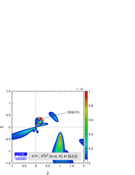
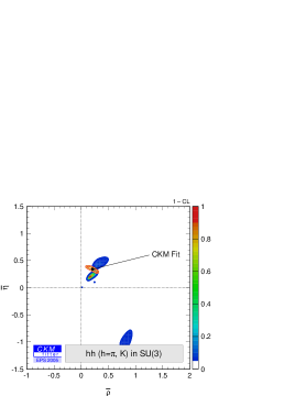
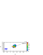
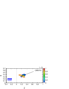
Figure 2: Top: constraints in the ($\overline{\rho}$,$\overline{\eta}$) plane from the joint “$\alpha$” and “$\beta$” subsystems (left) and for the full system (right). Bottom: constraints in the ($\overline{\rho}$,$\overline{\eta}$) plane for the full system with errors expected in 2008 including two B factories and CDF (left) and adding three inputs from LHCb (right).

5.3 Future physics potential

To estimate the future physics potential of this method, we have performed a tentative analysis using the errors expected in 2008. Central values have been chosen to be the best fit values for the current set of inputs in the full system framework. The two bottom plots of figure 2 show the induced constraints from a closest view in the ($\overline{\rho}$,$\overline{\eta}$) plane. On the left, two B factories with $1000fb^{-1}$ each have been considered $\!{}^{{\bf?}}$; and on the right, three inputs from LHCb have been added $\!{}^{{\bf?}}$ ($C^{+-}_{B_{s}\rightarrow KK}$, $S^{+-}_{B_{s}\rightarrow KK}$ and ${\cal A}^{+-}_{B_{s}\rightarrow K\pi}$). Including LHCb results, the contraints are found to be competitive with the current CKM fit demonstrating the predictive power of this framework.

6 Conclusion and outlook

Already with the limited set of observables currently available, significant constraints on the CKM parameters are obtained. Also, observables from the $B^{0}\rightarrow\pi^{+}\pi^{-}$, $B^{0}\rightarrow K^{+}\pi^{-}$, and $B^{0}\rightarrow K^{+}K^{-}$ subsystem alone are shown to bring strong constraints on the CKM angle $\alpha$. A similar constraint on $\beta$ is obtained from the subsystem $B^{0}\rightarrow\pi^{0}\pi^{0}$, $B^{0}\rightarrow K^{0}\pi^{0}$, and $B^{0}\rightarrow K^{+}K^{-}$. The full constraint on the apex on the Unitarity Triangle can already be compared with the standard CKM global fit. In the future, this framework alone will be able to determine the Unitarity Triangle with an accuracy comparable to the current CKM fit, and could be used to constraint SU(3) breaking or New Physics parameters.

References

- [1] J. Charles, J. Malclès, J. Ocariz, for the [CKMfitter Group], in preparation.
- [2] J. Charles et al. [CKMfitter Group], Eur. Phys. J. C 41, 1 (2005).
- [3] See Ref. [2] and references therein.
- [4] C. W. Bauer, I. Z. Rothstein and I. W. Stewart, hep-ph/0510241, (2005).
- [5] J. P. Silva and L. Wolfenstein, Phys. Rev. D 49, 1151 (1994).
- [6] M. Gronau and J. L. Rosner, Phys. Lett. B 572, 43 (2003).
- [7] A.J. Buras, R. Fleischer, S. Recksiegel and F. Schwab, Eur. Phys. J.C 32, 45 (2003).
- [8] A.J. Buras, R. Fleischer, S. Recksiegel and F. Schwab, Phys. Rev. Lett. 92, 101804 (2004); CERN-PH-TH-2004-020, hep-ph/0402112 (2004).
- [9] Y. L. Wu and Y. F. Zhou, Phys. Rev. D 72, 034037 (2005).
- [10] A. Buras and R. Fleischer, Eur. Phys. J. C 11, 93 (1999).
- [11] M. Neubert and J. Rosner, Phys. Lett. B 441, 403 (1998); Phys. Rev. Lett. 81, 5076 (1998).
- [12] G. Buchalla, A.J. Buras and M.E. Lautenbacher, Rev. Mod. Phys. 68, 1125 (1996).
- [13] A. Khodjamirian, T. Mannel and M. Melcher, Phys. Rev. D 68, 114007 (2003).
- [14] The Heavy Flavor Averaging Group (HFAG), http://www.slac.stanford.edu/xorg/hfag/.
- [15] A. Höcker, H. Lacker, S. Laplace and F. Le Diberder, Eur. Phys. J. C 21, 225 (2001).
- [16] P. Burchat et al. [BABAR Collaboration], BABAR analysis document #1228 (2005).
- [17] T. Nakada, A. Smith, W. Witzeling [LHCb Collaboration], CERN-LHCC-2003-030 (2003).