Generalized Emission Functions for Photon Emission from Quark-Gluon Plasma

Abstract

The Landau-Pomeranchuk-Migdal effects on photon emission from the quark gluon plasma have been studied as a function of photon mass, at a fixed temperature of the plasma. The integral equations for the transverse vector function (${\bf\tilde{f}(\tilde{p}_{\perp})}$) and the longitudinal function ($\tilde{g}({\bf\tilde{p}_{\perp}})$) consisting of multiple scattering effects are solved by the self consistent iterations method and also by the variational method for the variable set {$p_{0},q_{0},Q^{2}$}, considering the bremsstrahlung and the $\bf aws$ processes. We define four new dynamical scaling variables, $x^{b}_{T}$, $x^{a}_{T}$, $x^{b}_{L}$, $x^{a}_{L}$, for bremsstrahlung and aws processes and analyse the transverse and longitudinal components as a function of {$p_{0},q_{0},Q^{2}$}. We generalize the concept of photon emission function and we define four new emission functions for massive photon emission represented by $g^{b}_{T}$, $g^{a}_{T}$, $g^{b}_{L}$, $g^{a}_{L}$. These have been constructed using the exact numerical solutions of the integral equations. These four emission functions have been parameterized by suitable simple empirical fits. In terms of these empirical emission functions, the virtual photon emission from quark gluon plasma reduces to one dimensional integrals that involve folding over the empirical $g^{b,a}_{T,L}$ functions with appropriate quark distribution functions and the kinematic factors. Using this empirical emission functions, we calculated the imaginary part of the photon polarization tensor as a function of photon mass and energy.

Quark gluon plasma (QGP) state is expected to be formed in the relativistic heavy ion collisions. In order to identify the plasma or a de-confined state, one needs to study the physical processes in quark matter, that can distinctly and conclusively identify this state of matter, such as parton energy loss leading to jet suppression mechanism. In this context, electromagnetic processes such as photons and dilepton emission are also considered as important signals. Photons and dileptons are emitted at various stages during plasma evolution, for an overview one may see peitz ; gale ; rapp and the references therein. In depth study of photon emission processes in quark-gluon plasma were reported kapusta ; bair including processes also from hot hadron gas kapusta . In the formalism of hard thermal loops braaten (HTL) effective theory, the processes of bremsstrahlung brem and a crossed process of off-shell annihilation called ${\bf aws}$ bremaws ; ktkl contribute to photon emission at the two loop level. These two processes contribute at the leading order $O(\alpha\alpha_{s})$ owing to the collinear singularity that is regularized by the effective thermal masses. Higher loop multiple scatterings having a ladder topology also contribute at the same order as the one and two loop processes arnold1 ; arnold2 . These higher loop rescatterings, each giving finite decoherent correction to the two loop processes, need to be resummed. This resummation effectively implements the Landau-Pomarenchk-Migdal (LPM) effects landau1 ; landau2 ; migdal arising due to rescattering of quarks in the medium during the photon formation time. This results in an integral equation of a transverse vector function for the real photons. The photon emission rates are suppressed owing to the LPM effects arnold1 ; arnold2 . The LPM modification of the photon spectrum is important at very low photon energies or at high photon energies. For example, the bremsstrahlung radiation is strongly suppressed by almost $~{}80\%$ at very low $q_{0}/T$ values, whereas the photon emission from $\bf aws$ falls strongly for higher $q_{0}/T$ values arnold2 . Thus the rescattering corrections modify the two loop contributions for bremsstrahlung and $\bf aws$ processes at opposite ends of the photon spectrum for real photons.

I Emission of Real Photons

The photon production rates from bremsstrahlung and the $\bf aws$ processes considering the LPM effects are estimated by using Eq.1 arnold2 .

$${\cal R}_{b,a} = \frac{80\pi T^{3}\alpha\alpha_{s}}{(2\pi)^{3}9\kappa}\int dp_{0}\left[\frac{p_{0}^{2}+(p_{0}+q_{0})^{2})}{p_{0}^{2}(p_{0}+q_{0})^{2})}\right]\left[n_{f}(q_{0}+p_{0})\right.$$ (1)

$$\left.(1-n_{f}(p_{0}))\right]~{}\int\frac{\bf d^{2}\tilde{p}_{\perp}}{(2\pi)^{2}}2{\bf\tilde{p}_{\perp}\cdot\Re\tilde{f}(\tilde{p}_{\perp})}$$

$$2{\bf\tilde{p}_{\perp}} = i\delta\tilde{E}({\bf\tilde{p}_{\perp}}){\bf\tilde{f}}({\bf\tilde{p}_{\perp}})+$$ (2)

$$\int\frac{d^{2}{\bf\tilde{\ell}_{\perp}}}{(2\pi)^{2}}\tilde{C}({\bf\tilde{\ell}_{\perp}})\left[{\bf\tilde{f}}({\bf\tilde{p}_{\perp}})-{\bf\tilde{f}}({\bf\tilde{p}_{\perp}+\tilde{\ell}_{\perp}})\right]$$

$$\delta\tilde{E}({\bf\tilde{p}_{\perp}}) = \frac{q_{0}T}{2p_{0}(q_{0}+p_{0})}\left[\tilde{p}_{\perp}^{2}+\kappa\right]$$ (3)

$${\cal R}_{b,a} = {\cal C}_{k}\int dp_{0}\left[p_{0}^{2}+(p_{0}+q_{0})^{2})\right]\left[n_{f}(q_{0}+p_{0})\right.$$ (4)

$$\left.(1-n_{f}(p_{0}))\right]C_{g}g(x)$$

$$g(x) = g(p_{0},q_{0},\kappa,T)$$ (5)

$$x = \frac{1}{\kappa_{0}}\frac{q_{0}T}{p_{0}(p_{0}+q_{0})}$$ (6)

$${\cal C}_{k} = \frac{40\alpha\alpha_{s}T}{9\pi^{4}q_{0}^{2}}$$ (7)

$$\kappa_{0}=\frac{M_{\infty}^{2}}{m_{D}^{2}}~{}\mbox{and}~{}C_{g} = \frac{\kappa}{T}\left(\frac{\kappa_{0}}{\kappa}\right)^{-0.40}$$ (8)

$\Re{\bf\tilde{f}(\tilde{p}_{\perp})}$ in Eq.1 is the real part of a transverse vector function which consists of the LPM effects due to multiple scatterings. This can be taken as transverse momentum vector ${\bf(\tilde{p}_{\perp})}$ times a scalar function of transverse momentum ${\tilde{p}_{\perp}}$. The sign  $\tilde{}$  denotes the dimensionless quantities in units of Debye mass $m_{D}$ as defined in arnold2 . The function ${\bf\tilde{p}_{\perp}\cdot\Re\tilde{f}(\tilde{p}_{\perp})}$ is determined by the collision kernel ($\tilde{C}({\bf\tilde{q}_{\perp}})$) in terms of the AMY integral equation (Eq.2) and the energy function $\delta E$ (Eq.3). This was solved in arnold2 using the variational approach. We simplified this variational approach and extended to finite baryon density case svs1 . Moreover, we reported that the complex LPM effects can be very well reproduced by introducing the photon emission function $g(x)$ of dynamical variable $x$ svsprc . In terms of the single variable function $g(x)$ , the photon emission rates are estimated as shown in Eq.4. A figure for $g(x)$ function for real photons will be presented later (Fig.6).

II Emission of Virtial Photons

Processes that contribute to virtual photon emission in QGP at $\alpha\alpha_{s}$ order alther and the higher order corrections thoma were reported. The processes $q\bar{q}\rightarrow g\gamma^{*}$ , and $qg\rightarrow q\gamma^{*}$ contribute to photon polarization tensor at the order of $\alpha\alpha_{s}$ and appear as the one loop processes in HTL method. Further considering LPM effects, photon emission from QGP as a function of photon mass was also reported lpmdilep . For the case of virtual photons, these multiple scatterings modify the imaginary part of self energy as a function of photon energy and momentum both. It has been shown that the rescatterings modify the self energy at low $Q^{2}$, more importantly around the tree level threshold, $Q^{2}=4M_{\infty}^{2}$ lpmdilep . The dilepton emission rates are estimated in terms of the imaginary part of retarded photon polarization tensor, given by lpmdilep .

$$\frac{dN_{\ell^{+}\ell^{-}}}{d^{4}xd^{4}Q}=\frac{\alpha_{EM}}{12\pi^{4}Q^{2}(e^{q0/T}-1)}\Im\Pi_{R\mu}^{\mu}(Q)$$ (9)

For the case of virtual photon emission having small virtulaity, the transverse vector function is determined by the Eq.10 and the energy transfer $\delta{E}(({\bf{p}_{\perp}},p_{0},q_{0},Q^{2})$ given in Eq.11 lpmdilep . For virtual photons, the coupling of quarks to longitudinal mode must be considered. This results in a scalar function of ${\bf p_{\perp}}$ which is determined by an integral equation and collision kernel in Eq.12. For simplicity, henceforth I will refer to Eq.12 as AGMZ equation. An analytical form for the collision kernel was given in kernel , owing to which the photon emission rate calculations became easy. The $\delta{E}$ is an energy denominator and can be interpreted as inverse formation time of the photon. For the case of massive photon emission, this energy denominator is modified by replacing $M_{\infty}^{2}\rightarrow M_{\mbox{eff}}=M_{\infty}^{2}+\frac{Q^{2}}{q_{0}^{2}}{2p_{0}r_{0}}$. For $Q^{2}>4M_{\infty}^{2}$, this M${}_{\mbox{eff}}$ can vanish or even become negative.

$$2{\bf{p}_{\perp}} = i\delta{E}({\bf{p}_{\perp}},p_{0},q_{0},Q^{2}){\bf{f}}({\bf{p}_{\perp}})+g^{2}C_{F}T$$ (10)

$$\int\frac{d^{2}{\bf{\ell}_{\perp}}}{(2\pi)^{2}}{C}({\bf{\ell}_{\perp}})\left[{\bf{f}}({\bf{p}_{\perp}})-{\bf{f}}({\bf{p}_{\perp}+{\bf\ell}_{\perp}})\right]$$

$$\delta E({\bf{p}_{\perp}},p_{0},q_{0},Q^{2})=\frac{q_{0}}{2p_{0}r_{0}}\left[{\bf{p}_{\perp}^{2}}+M_{\mbox{eff}}^{2}\right]$$ (11)

$$2{\bf\sqrt{|p_{0}r_{0}|}} = i\delta{E}({\bf{p}_{\perp}},p_{0},q_{0},Q^{2})g({\bf{p}_{\perp}})+g^{2}C_{F}T$$ (12)

$$\int\frac{d^{2}{\bf{\bf\ell}_{\perp}}}{(2\pi)^{2}}C({\bf{\ell}_{\perp}})\left[g({\bf{p}_{\perp}})-g({\bf{p}_{\perp}+\bf{\ell}_{\perp}})\right]~{}~{}~{}~{}~{}$$

In above equations, $r_{0}=p_{0}+q_{0}$ and ${\bf{f}},g$ are actually functions of $p_{0},q_{0},Q^{2}$ represented as, ${\bf{f}}({\bf{p}_{\perp}},p_{0},q_{0},Q^{2})$, $g({\bf{p}_{\perp}},p_{0},q_{0},Q^{2})$. The Eq.10 and Eq.2 are identical except for $\delta E$ energy factor. Further, Eq.10 and the Eq.12 are also similar except for the left side of AGMZ equation is a constant $\sqrt{|p_{0}r_{0}|}$. Aurenche et. al., solved these equations, based on a very elegant method of impact parameter representation lpmdilep . As mentioned earlier, we have solved the AMY equation by the variational method and a new method called iterations method. These methods are formulated in terms of tilde variables. Therefore, it is required to transform the two above equations to tilde quantities. Following the definition of arnold2 we have,

$${\bf\tilde{p}_{\perp}}=\frac{\bf p_{\perp}}{m_{D}}~{};~{}{\bf\tilde{f}(\tilde{p}_{\perp})}=\frac{m_{D}}{T}{\bf{f}({p}_{\perp})}~{};~{}{\tilde{\delta E}}({\bf\tilde{p}_{\perp}})=\frac{T}{m_{D}^{2}}{\delta E(\bf{p}_{\perp}}).$$ (13)

One can see that the collision kernel are related by $\tilde{C}{\bf(\tilde{\bf\ell}_{\perp}})=TC({\bf\ell_{\perp}}).$

$$2{\bf\tilde{p}_{\perp}} = i\delta\tilde{E}({\bf\tilde{p}_{\perp}},p_{0},q_{0},Q^{2}){\bf\tilde{f}}({\bf\tilde{p}_{\perp}})$$ (14)

$$+\int\frac{d^{2}{\bf\tilde{\bf\ell}_{\perp}}}{(2\pi)^{2}}\tilde{C}({\bf\tilde{\ell}_{\perp}})\left[{\bf\tilde{f}}({\bf\tilde{p}_{\perp}})-{\bf\tilde{f}}({\bf\tilde{p}_{\perp}+\tilde{\bf\ell}_{\perp}})\right]$$

$$\delta\tilde{E}({\bf\tilde{p}_{\perp}},p_{0},q_{0},Q^{2})=\frac{q_{0}T}{2p_{0}(q_{0}+p_{0})}\left[\tilde{p}_{\perp}^{2}+\kappa_{\mbox{\small{eff}}}\right]$$ (15)

In above $\kappa_{\small{\mbox{eff}}}=\frac{M^{2}_{\mbox{\small{eff}}}}{m_{D}^{2}}$. In the equations below, we introduce the calligraphic symbol $\cal{C}$ which is is a linear operator and this should not be confused with the collision kernel $C(\bf{p_{\perp}})$. The integral equations can be put in the following linear operator form.

$$2{\bf\tilde{p}_{\perp}} = \left(i\delta\tilde{E}({\bf\tilde{p}_{\perp}})+\tilde{\cal{C}}({\bf\tilde{p}_{\perp}})\right){\bf\tilde{f}}$$ (16)

$$\tilde{\cal{C}}({\bf\tilde{p}_{\perp}}){\bf\tilde{f}} = \int\frac{d^{2}{\bf\tilde{\bf\ell}_{\perp}}}{(2\pi)^{2}}\tilde{C}({\bf\tilde{\ell}_{\perp}})\left[{\bf\tilde{f}}({\bf\tilde{p}_{\perp}})-{\bf\tilde{f}}({\bf\tilde{p}_{\perp}+\tilde{\bf\ell}_{\perp}})\right]~{}~{}~{}~{}~{}$$ (17)

The linear operator at a given momentum ${\bf{p_{\perp}}}$ gives the sum of the transverse vector function differences between the current momentum and all other momenta arising from scattering weighted by collision kernel. The above linear operator suggests that the corresponding tilde operator is related to untilded operator exactly as the $\delta E$ operator. It can be easily verified that for the transverse equation this means, $\tilde{\cal{C}}({\bf\tilde{p}_{\perp}})=(T/m_{D}^{2})\cal{C}({\bf p}_{\perp})$. In the AGMZ equation when $\delta E$ transforms to tilde quantity, its $T/m_{D}^{2}$ factor has to be absorbed by the transformation of $g$ function. Therefore, if we set the $g$ to transform as $\tilde{g}({\bf\tilde{p}_{\perp}})=\frac{m_{D}^{2}}{T}g({\bf p_{\perp}})$, the equation for the longitudinal part could be written as,

$$2{\sqrt{|p_{0}r_{0}|}} = i\delta\tilde{E}({\bf\tilde{p}_{\perp}},p_{0},q_{0},Q^{2}){\tilde{g}}({\bf\tilde{p}_{\perp}})+$$ (18)

$$\int\frac{d^{2}{\bf\tilde{\ell}_{\perp}}}{(2\pi)^{2}}\tilde{C}({\bf\tilde{\ell}_{\perp}})\left[{\tilde{g}}({\bf\tilde{p}_{\perp}})-{\tilde{g}}({\bf\tilde{p}_{\perp}+\tilde{\bf\ell}_{\perp}})\right]~{}~{}~{}~{}~{}$$

This implies that the $\tilde{g}$ is larger than $g$ by a factor $m_{D}^{2}$. Therefore, when the solution for this Eq.18 is obtained and integrated over $\int\frac{d^{2}\bf\tilde{p}_{\perp}}{(2\pi)^{2}}\Re{\tilde{g}{\bf(\tilde{p}_{\perp})}}$, the result will be larger than the true result by exactly $m_{D}^{2}$ factor. This problem was not present for the transverse part because $\bf{p_{\perp}.f(p_{\perp})}$ is independent of any $m_{D}^{2}$ factor arising from the tilde transformation. Therefore, to take this anomaly into account correctly, we will introduce $\frac{1}{m_{D}^{2}}$ factor for the longitudinal contribution while estimating the imaginary part of photon polarization tensor. Further, in the tilde variables, the above equation is not dimensionless. Therefore, we will divide the above Eq.18, by $m_{D}$ in order to get the following equation, where absorbing 1/$m_{D}$ factor, $g$ is now re-defined.

$$2\sqrt{\frac{|p_{0}r_{0}|}{m_{D}^{2}}} = i\delta\tilde{E}(({\bf\tilde{p}_{\perp}},p_{0},q_{0},Q^{2}){\tilde{g}}({\bf\tilde{p}_{\perp}})+$$ (19)

$$\int\frac{d^{2}{\bf\tilde{\ell}_{\perp}}}{(2\pi)^{2}}\tilde{C}({\bf\tilde{\ell}_{\perp}})\left[{\tilde{g}}({\bf\tilde{p}_{\perp}})-{\tilde{g}}({\bf\tilde{p}_{\perp}+\tilde{\bf\ell}_{\perp}})\right]~{}~{}~{}~{}~{}$$

In the above equation, $g$ transforms as $\tilde{g}({\bf\tilde{p}_{\perp}})=\frac{m_{D}}{T}g({\bf p_{\perp}})$, similar to $\bf f(p_{\perp})$ function. Therefore, the anomalous factor is now $\frac{1}{m_{D}}$. In the present work, we have solved the above Eq.19 by iterations and variational method. The variational method for longitudinal part has been re-derived svssymp . We could get good agreement of distributions form iterations method and variational results and these details will be discussed elsewhere. Following these two methods, we obtained the $\bf p_{\perp}$ distributions for the bremsstrahlung and aws cases for both transverse and longitudinal components. We considered five photon energy values, for each energy ten photon momenta and ten quark momenta, a total of 500 distributions for transverse and longitudinal components of bremsstrahlung. Similarly the distributions were obtained for aws case. All these were compared in both iterations and variational method.

III Empirical Analysis of the Solutions of AMY, AGMZ integral equations

In all the calculations that follow, we have used two flavors, three colors and $\alpha_{s}$=0.30 and T=1.0GeV. In Eqs.20-23 we define four dimensionless variables used in the following work. Here one may notice that the variable $x_{1}$ is the inverse of $x$ variable used in svsprc for real photon production. $I^{b,a}_{T,L}$ are defined in the Eqs.24,25 which are obtained by integrating the ${\bf p_{\perp}.f(p_{\perp})},g({\bf p_{\perp}})$ distributions ( in Ref.svsprc there was a 2 factor extra in the definition of $I$ as given by ${\bf 2p_{\perp}.f(p_{\perp})}$ ). $I^{b,a}_{T,L}$ are the quantities required for imaginary part of polarization tensor and the rate equations.

$$x_{0} = \frac{|(p_{0}+q_{0})p_{0}|}{q_{0}T}$$ (20)

$$x_{1} = x_{0}\frac{M_{\infty}^{2}}{m_{D}^{2}}$$ (21)

$$x_{2} = x_{0}\frac{Q^{2}}{q_{0}T}$$ (22)

$$x_{3} = \frac{q_{0}T}{Q^{2}}$$ (23)

$$I^{b,a}_{T} = \int\frac{\bf d^{2}\tilde{p}_{\perp}}{(2\pi)^{2}}{\bf\tilde{p}_{\perp}\cdot\Re\tilde{f}(\tilde{p}_{\perp})}$$ (24)

$$I^{b,a}_{L} = \int\frac{\bf d^{2}\tilde{p}_{\perp}}{(2\pi)^{2}}\Re\tilde{g}({\bf\tilde{p}_{\perp})}$$ (25)

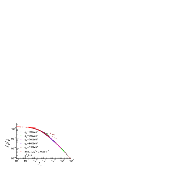
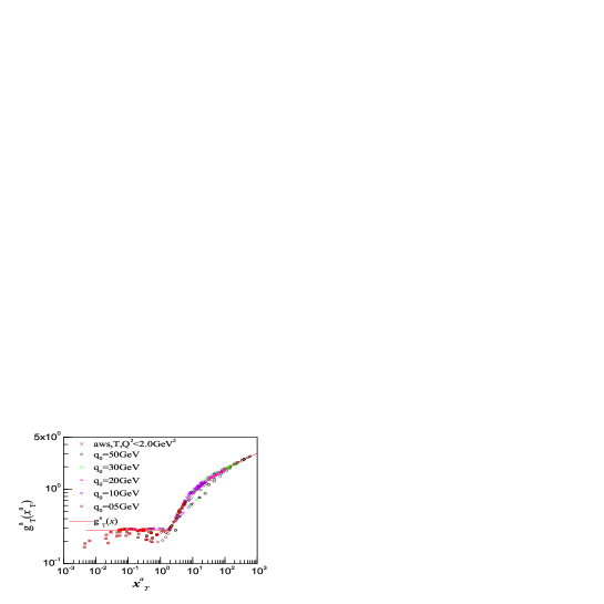
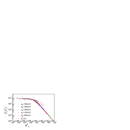
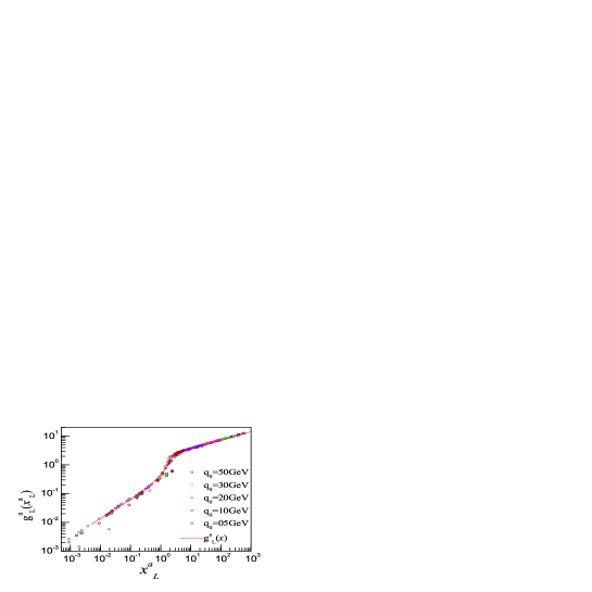
In the above equations superscript $b,a$ represent bremsstrahlung or $\bf aws$ processes depending on the $p_{0}$ value used. The subscripts $T,L$ represent contributions from transverse ($\bf f(p_{\perp})$) or longitudinal $(g(\bf p_{\perp}))$parts. Using the iterations data, we first obtained the integrated values of ${\bf p_{\perp}}$ distributions as given by $I^{b,a}_{T,L}$ of Eqs.24,25. We define the emission functions $g^{b,a}_{T,L}$ in Eq.26 which are functions of variables $x^{b,a}_{T,L}$. These $x^{b,a}_{T,L}$ variables are given in Eqs.27-30. The $g^{b,a}_{T,L}$ are obtained from corresponding $I^{b,a}_{T,L}$ values by multiplying with $c^{b,a}_{T,L}$ coefficient factors which are given in Eqs.31-34. Therefore, using the $I^{b,a}_{T,L}$ obtained from iterations and variational data, we constructed all the four $g^{b,a}_{T,L}$ in Eq.26. It should be noted that the quantities $x^{b,a}_{T,L}$ and $c^{b,a}_{T,L}$ listed in Eqs.27-34 are not definitions. They are the results of a hard search for dynamical variables hidden in the solutions of AMY and AGMZ equations.

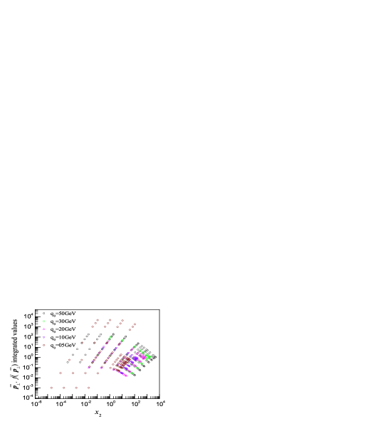
Figure 1: The integrated values $I^{b}_{T}(x)$ versus dynamical variable $x_{2}$ defined in the text. The symbols represent the integrated values of ${\bf p_{\perp}}$ distributions of about 500 cases of $\{p_{0},q_{0},Q^{2}\}$ values. The different colored symbols represent different photon energies.

Figure 2: The dimensionless emission function $g^{b}_{T}(x)$ versus dynamical variable $x^{b}_{T}$ defined in the text. The symbols represent the integrated values of ${\bf p_{\perp}}$ distributions of about 500 cases of $\{p_{0},q_{0},Q^{2}\}$ values and are transformed by suitable $c^{b}_{T}$ coefficient functions. The different colored symbols represent different photon energies. The red curve is an empirical fit given in the text.

Figure 3: The dimensionless emission function $g^{a}_{T}(x)$ versus dynamical variable $x^{a}_{T}$ defined in the text. The required $c^{a}_{T}$ are the transformation coefficients and empirical fit (red curve) are given in the text.

Figure 4: The dimensionless emission function $g^{b}_{L}(x)$ versus dynamical variable $x^{b}_{L}$ defined in the text. The required $c^{b}_{L}$ are the transformation coefficients and empirical fit (red curve) are given in the text.

Figure 5: The dimensionless emission function $g^{a}_{L}(x)$ versus dynamical variable $x^{a}_{L}$ defined in the text. The required $c^{a}_{L}$ are the transformation coefficients and empirical fit (red curve) are given in the text.

$$g^{b,a}_{T,L}(x^{b,a}_{T,L}) = I^{b,a}_{T,L}(x^{b,a}_{T,L})c^{b,a}_{T,L}$$ (26)

$$x^{b}_{T} = x_{2}+x_{1}$$ (27)

$$x^{a}_{T} = x_{2}+0.18x_{1}$$ (28)

$$x^{b}_{L} = x_{2}$$ (29)

$$x^{a}_{L} = x_{2}$$ (30)

$$c^{b}_{T} = \frac{1}{x_{1}^{2}}$$ (31)

$$c^{a}_{T} = \frac{1}{x_{1}\left(1.0+x_{3}^{0.85}\right)x_{2}^{0.8}}$$ (32)

$$c^{b}_{L} = \frac{Q^{2}}{(p_{0}(p_{0}+q_{0}))^{1.50}}\left(1.50+x_{3}^{0.75}\right)/x_{2}^{1/3}$$ (33)

$$c^{a}_{L} = \frac{1}{x_{1}^{1.4}q_{0}^{0.5}\left(1+x_{3}^{0.5}\right)}x_{2}^{0.2}$$ (34)

Figure 1 shows the $I^{b}_{T}(x)$ as a function of $x_{2}$ variable. All the bremsstrahlung transverse mode data consisting of about 500 points are shown in the figure. The figure exhibits some trends as a function of $p_{0},q_{0},Q^{2}$ values, but still does not bring out the underlying dynamical scale hidden in the data. When plotted with respect to any other variables, the representation is much worse and no trend emerges from such plots. In Figure 2, we show the same data transformed to $g^{b}_{T}(x^{b}_{T})$ as a function of $x^{b}_{T}$ variable which is a combination of $x_{2}$ and $x_{1}$ variables. The hidden scale is revealed in this plot, where data for all different $p_{0},q_{0},Q^{2}$ values merged into a single curve. Colored symbols represent different photon energies. This is the transverse mode bremsstrahlung emission function. Importantly, the crosses in the figure represent low $Q^{2}$ data for transverse mode of the ${\bf aws}$ process, intentionally plotted over here and will be explained in the next figure. We have obtained an empirical fits to this data as given by $g^{b}_{T}(x)(empirical)$ formula in Eq.35. The need for the empirical fit will become clear later.

$$g^{b}_{T}(x) = \frac{10.0}{5.0+3.0\sqrt{x}+x}$$ (35)

$$g^{a}_{T}(x) = a+bx^{p}$$ (36)

$$a = -4.1395~{};~{}b=4.1818~{};~{}p=0.0779$$

$$g^{a}_{T} = 0.28~{}~{}~{}\mbox{if}~{}~{}~{}g^{a}_{T}(x)<0.28$$

$$g^{b}_{L}(x) = \frac{0.0876}{1+\left(\frac{x}{3.7727}\right)^{1.18}}$$ (37)

$$g^{a}_{L}(x) = 0.2703x^{0.65}+0.20x^{2}$$ (38)

$$\mbox{if}~{}x > 2.5~{}\mbox{then}~{}g^{a}_{L}(x)=1.8x^{0.3}$$

$$I^{b,a}_{T,L} = \frac{g^{b,a}_{T,L}(x)}{c^{b,a}_{T,L}}$$ (39)

Similar exercise for transverse ${\bf aws}$ is shown in Figure 3. However, we notice that the $x$ variable is different from the previous figure. Further, the $c^{a}_{T}$ that transform the integrated values into $g$ functions are very complex. We have parameterized this data by an empirical function given in Eq.36. One important thing to notice is for low enough $Q^{2}<4.0GeV$ (possibly the data for $Q^{2}<4M_{\infty}^{2}$), the data deviates from general trends. These low $Q^{2}$ data is shown by crosses in the figure. It was noticed that the same data when transformed as required in Fig.2 and plotted versus $x^{b}_{T}$, they are very close to the bremsstrahlung function. This is shown by crosses in the previous figure (Fig.2). Therefore, the transverse mode emission functions for the bremsstrahlung and for the low $Q^{2}$ ${\bf aws}$ are the same and are given by $g^{b}_{T}(x^{b}_{T})$(empirical).
The Figure 4 shows the results for bremsstrahlung longitudinal component. The corresponding $c^{b}_{L}$ coefficient functions and the empirical fits represented by $g^{b}_{L}(x)$ are given in Eqs.33,37. Similarly, the Figure 5 shows the results for aws longitudinal component. The corresponding $c^{a}_{L}$, $g^{a}_{L}(x)$ are given in Eqs.34,38.

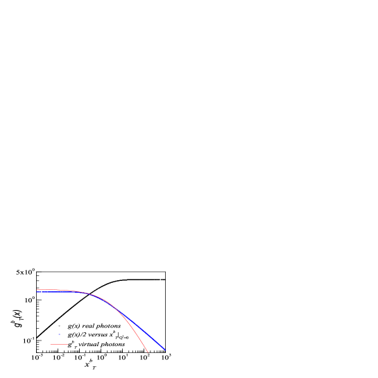
Figure 6: The dimensionless emission function $g(x)$ versus dynamical variable $x$ taken from svsprc , represented by black symbols. The half value of this $g(x)$ in the inverse scale (that is same as present $x_{1}$ variable) is shown by blue symbols. This inverse variable coincides with the present $x^{b}_{T}$ when $Q^{2}\rightarrow 0$. The results for transverse mode of the virtual photon case versus $x^{b}_{T}$ variable is shown by the red curve (same as in Fig.2).

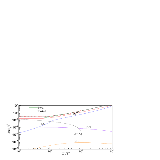
Figure 7: $\Im\Pi_{R}$ plotted as a function of $Q^{2}/T^{2}$ for a photon energy of 50GeV. The transverse components of bremsstrahlung, $\bf aws$, the insignificant contribution from longitudinal parts, and the $2\rightarrow 2$ processes contribution using the Eq.42 are all shown. The purpose of the figure is to test our empirical method compared to the results of Fig.3 of Aurenche et. al.,lpmdilep shown by red circles.

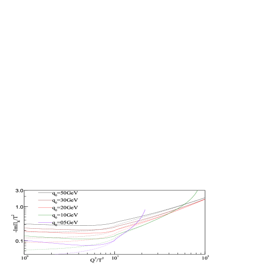
Figure 8: Imaginary part of retarded photon polarization tensor for five photon energies represented by dashed curves in various colors obtained from the empirical emission functions. After adding the $2\rightarrow 2$ contribution from Eq.42, the results are shown by colored solid curves.

In Figure 6, we show the photon emission function in terms of dynamical variable $x$ versus $g(x)$ defined and shown in Ref.svsprc for real photons. We reproduce that data in the Figure. 6 represented by black symbols. The inverse of this $x$-variable of svsprc coincides with the present $x_{1}$ value and is related to the variables of the present study by $x^{-1}$(of Ref.svsprc )=$x^{b}_{T}\left|{}_{Q^{2}\rightarrow 0}\right.$. This is the motivation for choosing the combination of $x_{1}$ and $x_{2}$ variables for transverse modes in the present study;  as $Q^{2}\rightarrow 0$, the dynamical variables of the transverse parts go over to real photon dynamical variable. Such a need is not there for longitudinal components. Further, the $g(x)$ defined in svsprc is two times larger than the definition in the present work for transverse modes (see factor 2 in $2{\bf p_{\perp}.f(p_{\perp})}$ in Eq.1 and not in Eqs.24,25). Therefore the rescaled $\frac{1}{2}g(x)$ versus $x^{-1}(=x^{b}_{T}\left|{}_{Q^{2}=0}\right.$) for real photons is also plotted in the figure by blue symbols. For comparison, the results of our present work for $g^{b}_{T}$ versus $x^{b}_{T}$ are also shown in the figure by red curve. This red curve is the same red curve shown in Fig.2, given by $g(x)=10.0/\left(5+3\sqrt{x}+x\right)$. It should be noted that in this figure, the variable for $x-axis$ is different for all the three curves. Further, we explained earlier, that for $Q^{2}<4.0GeV^{2}$, the transverse component of the $\bf aws$ data lies very close to the bremsstrahlung curve (see crosses in the figure 2). From these results it is obvious that for small quark momenta and low virtuality of the photons emitted, the transverse part of the virtual photon ($\gamma^{*}$) emission function and real photon ($\gamma$) emission functions are the same as given by, $g^{b}_{T}(x^{b}_{T})(\gamma^{*})\approx g(x)(\gamma)$ and this $x$ for real photons is simply $x=x^{b}_{T}\left|{}_{Q^{2}=0}\right.$. Further, the other longitudinal components for virtual photons are all negligible. Therefore, for high photon energies and small photon virtualities, the virtual photon emission is identical to real photons emission in the sense that their emission functions are the same.

IV Empirical Estimation of Photon Retarded Polarization Tensor

The imaginary part of retarded photon polarization tensor can be calculated using the $\bf p_{\perp}$ integrated values as shown in Eq.40. In the previous section, we used the results from variational and iterations methods to obtain the $I^{b,a}_{T,L}$ values by integrating the distributions. We transformed these into $g^{b,a}_{T,L}$ functions shown in Figs.2-5 and we fitted these by empirical functions Eqs.35-38. The need for fitting arises, for example, for any $\{p_{0},q_{0},Q^{2}\}$ values, we can generate the integrated values $I^{b,a}_{T,L}(x)$ as given by Eq.39, without solving integral equations. The imaginary part of retarded photon polarization tensor (in units of $T^{2}$ and represented by $\Im\Pi_{R}$) is calculated, as in Eq.41. Note that in this section, no data from variational method or iterations is used. The empirical fit functions provide the required results circumventing the need to solve the transverse and longitudinal integral equations. The imaginary part of $\Pi_{R}$ has $\frac{Q^{2}}{q^{2}}$ factor for longitudinal part and this diverges as $Q^{2}\rightarrow q_{0}^{2}$. This trend is seen in the Figs.7,8 as $Q^{2}$ increases. In this Eq.41, one should note the multiplying factor $\left(80\alpha_{s}\kappa/3\pi\right)$, in the present work it is equal to $\frac{2}{\pi}$. Importantly, one should note the factor $\frac{1}{m_{D}}$ in the longitudinal part. This is because the $\tilde{g}$ is already rescaled in Eq.19. In Eq.41 the superscript $i$ denotes $\{b,a\}$ bremsstrahlung and annihilation depending on the value of the integration variable $p_{0}$. All terms in this equation are calculated and plotted in Fig.7 to show the contribution to polarization tensor.

$$\Im{\Pi^{\mu}}_{R\mu} = \frac{e^{2}N_{c}}{2\pi}\int_{-\infty}^{\infty}dp_{0}[n_{F}(r_{0})-n_{F}(p_{0})]\otimes$$ (40)

$$\int\frac{d^{2}{\bf\tilde{p}_{\perp}}}{(2\pi)^{2}}\left[\frac{p_{0}^{2}+r_{0}^{2}}{2(p_{0}r_{0})^{2}}\Re{\bf\tilde{p}_{\perp}.\tilde{f}(\tilde{p}_{\perp})}+\right.$$

$$\left.\frac{1}{\sqrt{\left|p_{0}r_{0}\right|}}\frac{Q^{2}}{q^{2}}\Re\tilde{g}({\bf\tilde{p}_{\perp}})\right]$$

$$\Im{\Pi^{\mu}}_{R\mu} = \frac{e^{2}N_{c}}{2\pi}\int_{-\infty}^{\infty}dp_{0}[n_{F}(r_{0})-n_{F}(p_{0})]\otimes$$ (41)

$$\left(\frac{2}{\pi}\right)\left[\frac{p_{0}^{2}+r_{0}^{2}}{2(p_{0}r_{0})^{2}}\left(\frac{g^{i}_{T}\left(x^{i}_{T}\right)}{c^{i}_{T}}\right)+\right.$$

$$\left.\frac{1}{\sqrt{\left|p_{0}r_{0}\right|}}\frac{Q^{2}}{q^{2}}\left(\frac{1}{m_{D}}\right)\left(\frac{g^{i}_{L}\left(x^{i}_{L}\right)}{c^{i}_{L}}\right)\right]$$

The contribution of oneloop processes to imaginary part of the photon polarization tensor is given by equation below (formula taken from lpmdilep ). We will use this formula to evaluate the contribution of one loop processes and add to our empirical result to obtain the total result for retarded photon polarization tensor.

$$Im{\Pi_{R}}^{\mu}_{\mu}\left|{}_{2\rightarrow 2}\right. = -\frac{e^{2}g^{2}N_{c}C_{F}T^{2}}{16\pi}\left[ln\left(\frac{2q_{0}T}{Q^{2}}\right)\right.$$ (42)

$$\left.+1+\frac{ln(2)}{3}-\gamma_{E}+\frac{\zeta^{\prime}(2)}{\zeta(2)}\right]$$

Figure 7 shows the $\Im\Pi_{R}$ plotted as a function of $Q^{2}/T^{2}$ for a photon energy of 50GeV. This figure has been compared with the results of Fig.3 of lpmdilep represented by red symbols (approximately) for testing our empirical approach. It can be seen that the empirical approach has predicted rather remarkably well the the results of lpmdilep over the $Q^{2}/T^{2}$ in the range of  $1-100$. Further, the polarization tensor increases rapidly with $Q^{2}/T^{2}$ beyond 100.0 The bremsstrahlung is insignificant obviously because the $q_{0}$ is very high. The transverse component of $\bf aws$ only contributes, with a small contribution from longitudinal component above $Q^{2}>20GeV^{2}$. The $2\rightarrow 2$ processes contribution is calculated using the Eq.42. The modification of the imaginary part of photon polarization tensor due to multiple re-scatterings in the medium has been well discussed in lpmdilep . The LPM effects only marginally increase the $\Im\Pi_{R}$ at low $Q^{2}$. Here $2\rightarrow 2$ processes also contribute. Importantly, the rescattering corrections smooth out the discontinuity at the threshold $Q^{2}=4M_{\infty}^{2}$. In order to understand how $\Im\Pi_{R}$ behaves with photon energy, we have calculated this quantity using empirical approach for five photon energies. These results are shown in Figure 8. The dashed curves are the results from present calculations. When $2\rightarrow 2$ contributions are added to this, we get the solid curves.

V Conclusion

The photon emission rates from the quark gluon plasma have been studied as a function of photon mass, considering LPM suppression effects at a fixed temperature. Self-consistent iterations method and the variational method have been used to solve the AMY and AGMZ integral equations. We obtained the ${\bf\Re\tilde{f}}({\bf\tilde{p}_{\perp}})$, ${\Re\tilde{g}}({\bf\tilde{p}_{\perp}})$ distributions as a function of photon mass, photon energy and quark momentum. The integrated values of these distributions for bremsstrahlung and $\bf aws$ show a very good scaling in terms of different dynamical variables for these two processes. We defined four new dynamical variables $x^{b}_{T},x^{b}_{L},x^{a}_{T},x^{a}_{L}$ for transverse and longitudinal components of bremsstrahlung and $\bf aws$ mechanism. In addition, we defined four new emission functions namely $g^{b}_{T}(x^{b}_{T})$,$g^{a}_{T}(x^{a}_{T})$,$g^{b}_{L}(x^{b}_{L})$$g^{a}_{L}(x^{a}_{L})$, that describe the photon emission for these four components. We have obtained empirical fits to these emission functions that have been constructed using the exact numerical calculations. In terms of the new emission functions, estimation of the imaginary part photon polarization tensor reduces to one dimensional integrals. Using this empirical approach, we have calculated the imaginary part of retarded photon polarization tensor as a function of photon energy and mass. These self energy graphs inlcude the LPM effects due to rescattering in the plasma medium. For small photon $Q^{2}$ values and high photon energies, the virtual photon emission function is a single function coinciding with the real photon emission function.