PQCD Calculation for $\Lambda_{b}\rightarrow\Lambda\gamma$ in the Standard Model

PACS numbers: 13.30.Ce, 12.38.Bx, 14.20.Mr

I Introduction

Rare radiative processes involving $b\to s\gamma$ at quark level are important for understanding the flavor changing structure in the standard model (SM). Exclusive radiative $B$ decays also provide important information about the hadronic matrix elements where a heavy b-quark is involved. These processes being rare can also provide clues to models beyond the SM. There have been considerable studies on inclusive $b\to s\gamma$CLEO ; b to s gamma exp , and exclusive mesonic $B\to K^{*}\gamma$exclusive gamma exp both experimentally and theoretically within and beyond the SM b to s gamma th ; exclusive gamma th ; newbgamma . Theoretical predictions for inclusive decays agree with data very well in the SM. Calculations for exclusive processes are in general consistent with data although there are unavoidable uncertainties due to our lack of good understanding of QCD at low energies. Nevertheless methods have been developed to calculate hadronic matrix elements in recent years hadronmesonBeneke ; hadronmesonLi . With more data becoming available, new b-decay processes can be studied. These processes can be new tests for different methods in calculating hadronic matrix elements and new physics beyond the SM. In this work we study $\Lambda_{b}\to\Lambda\gamma$. In this decay more experimental information about the heavy b quark inside the hadron which is not available in inclusive and mesonic b-hadron decays, such as spin polarization during hadronization, and the handedness of the couplings at the quark level, can be extractedllll ; Mannel ; Huang ; Mohanta ; Cheng . Therefore the baryonic b-hadron radiative decay can provide a new test for theoretical methods for b-quark hadronization.

There are some studies in the literature on $\Lambda_{b}\to\Lambda\gamma$llll ; Mannel ; Huang ; Mohanta ; Cheng decay ranging from phenomenological models to QCD sum rule approaches. Our study will be based on the PQCD methodLip ; Lic ; LiJ . This method has been shown to give consistent results for two body mesonic B decayshadronmesonLi . We expect a PQCD calculation for $\Lambda_{b}\to\Lambda\gamma$ will also give a reasonable estimate since the energy-exchange carried by gluons in the matrix element calculations is large. Result obtained in this way can serve as a good reference for discussing the relevant hadronic matrix elements.

For SM, the effective Hamiltonian responsible for $b\to s\gamma$ comes from the electromagnetic penguin diagram and is given byH :

$$H_{eff} = i\frac{G_{F}}{2\sqrt{2}}V_{tb}V_{ts}^{*}{e\over 4\pi^{2}}C^{eff}_{7}(\mu)m_{b}\bar{s}\sigma_{\mu\nu}(1+\gamma_{5})bF^{\mu\nu},$$ (1)

where $C_{7}^{eff}(\mu=m_{b})=-0.31$. In our numerical calculations, the running of $C_{7}^{eff}$ will also be taken into account.

It has been shown that there may be resonant (long distance) $J/\psi(\psi^{\prime})$ contributionslong0 . If these contributions are included, one should add a term $(3C_{1}(\mu)+C_{2}(\mu))(3/\alpha_{em}^{2})\sum_{j=\psi,\psi^{\prime}}\omega_{j}(0)k_{j}\pi\Gamma(j\rightarrow l^{+}l^{-})M_{j}/(q^{2}-M_{j}^{2}+iM_{j}\Gamma_{j}^{tot})$ to the Wilson coefficient $C^{eff}_{7}$. Since for $b\to s\gamma$ process, $q^{2}=0$, there are double suppressions for the long distance resonant contributions with one of them coming from the Breit-Wigner factor $\sim\Gamma_{i}/M_{i}$ and another coming from the extrapolation of $\omega_{j}(M^{2}_{i})=1$ to $\omega_{j}(0)$ with $\omega_{j}(0)<0.13$ (and could be smaller)long0 , we will neglect the resonant contribution for radiative decays in our later discussions.

At the hadron level, the decay amplitude for $\Lambda_{b}\to\Lambda\gamma$ is obtained by inserting the effective Hamiltonian between the initial and final hadron states,

$$M(\Lambda_{b}\to\Lambda\gamma)=\langle\Lambda\gamma|H_{eff}|\Lambda_{b}\rangle.$$ (2)

There are two form factors for $\Lambda_{b}\to\Lambda\gamma$ from the above which we write as

$$M_{\mu} \equiv\langle\Lambda(p^{\prime})|C_{7}^{eff}(\mu,0)\bar{s}\sigma_{\mu\nu}q^{\nu}(1+\gamma_{5})b|\Lambda_{b}(p)\rangle=\overline{\Lambda(p^{\prime})}(F_{L}\sigma_{\mu\nu}q^{\nu}(1-\gamma_{5})+F_{R}\sigma_{\mu\nu}q^{\nu}(1+\gamma_{5}))\Lambda_{b}(p).$$ (3)

We obtain

$$\Gamma(\Lambda_{b}\to\Lambda\gamma)={G_{F}^{2}|V_{tb}|^{2}|V_{ts}|^{2}\alpha_{em}|C_{7}^{eff}|^{2}m_{b}^{2}\over 32m_{\Lambda_{b}}^{3}\pi^{4}}(m_{\Lambda_{b}}^{2}-m_{\Lambda}^{2})^{3}(|F_{L}|^{2}+|F_{R}|^{2}).$$ (4)

Emission of a photon from the tree operators $O_{1,2}$ can also contribute to $\Lambda_{b}\to\Lambda\gamma$. Although the Wilson coefficients of these operators are larger than those of the penguin operators, there is a large suppression coming from the CKM factor $|V_{ub}V_{us}^{*}/V_{tb}V_{ts}^{*}|$. The overall contributions from bremsstrahlung of a photon off the operator $O_{1,2}$ is therefore suppressed. We will neglect their contribution in rest of discussions.

II PQCD calculation of the hadronic matrix elements

We now describe our calculations for the hadronic matrix elements defined above using the PQCD method developed in Ref.Lip ; Lic ; LiJ . We define, in the rest frame of $\Lambda_{b}$, $p$, $p^{\prime}$ to be the $\Lambda_{b}$, $\Lambda$ momenta, $k_{i}(i=1,2,3)$ to be the valence quark momenta inside $\Lambda_{b}$, and $k_{i}^{\prime}$ to be the valence quark momenta inside $\Lambda$. We parameterize the light cone momenta with all light quark and baryon masses neglected as

$$p=(p^{+},p^{-},\mathbf{0}_{T})=\frac{M_{\Lambda_{b}}}{\sqrt{2}}(1,1,\mathbf{0}_{T}),\;\;p^{\prime}=(p^{\prime+},0,\mathbf{0}_{T})$$

$$k_{1}=(p^{+},x_{1}p^{-},\textbf{k}_{1T}),\;\;k_{2}=(0,x_{2}p^{-},\textbf{k}_{2T}),\;\;k_{3}=(0,x_{3}p^{-},\textbf{k}_{3T})$$

$$k^{\prime}_{1}=(x_{1}^{\prime}p^{\prime+},0,\textbf{k}_{1T}^{\prime}),\;\;k^{\prime}_{2}=(x_{2}^{\prime}p^{\prime+},0,\textbf{k}_{2T}^{\prime}),\;\;k^{\prime}_{3}=(x_{3}^{\prime}p^{\prime+},0,\textbf{k}_{3T}^{\prime})$$ (5)

where $x_{i}$ and $x^{\prime}_{i}$ are the fractions of the longitudinal momenta of the valence quarks with $x_{1}+x_{2}+x_{3}=1$ and $x^{\prime}_{1}+x^{\prime}_{2}+x^{\prime}_{3}=1$. $\mathbf{k}_{iT}$ and $\mathbf{k}_{iT}^{\prime}$ are the transverse momenta of the valence quarks inside $\Lambda_{b}$ and $\Lambda$, respectively.

As a self-consistent check, one should make sure that the expected relation $p^{2}-k_{1}^{2}\sim 0(\Lambda_{QCDm_{b}})$ holds, since the light quarks in the heavy baryon should have momenta of order $\Lambda_{QCD}$. Naively, the above gives a value of order $(1-x_{2})m^{2}_{\Lambda_{b}}$ which does not have the explicit form as expected. To understand this, one needs to combine the form of the heavy baryon wavefunction which determines how quark momenta are distributed inside the baryon. We have checked this using the wavefunction given later, and obtained the ratio of average values $<x_{2,3}>/<x_{1}>\sim m/m_{\Lambda_{b}}$, where $m$ is of order $\Lambda_{QCD}$. With the constraint $x_{1}+x_{2}+x_{3}=1$, the desired order for $p^{2}-k^{2}_{1}$ is then obtained.

One can write $p^{\prime+}=\rho p^{+}$ with $\rho=\frac{2p\cdot p^{\prime}}{M_{\Lambda_{b}}^{2}}={p^{2}+p^{\prime 2}-q^{2}\over M_{\Lambda_{b}}^{2}}$. The ranges for $q^{2}$ and $\rho$ are given by $0\leq q^{2}\leq(M_{\Lambda_{b}}-m_{\Lambda})^{2}$ and ${2m_{\Lambda}/M_{\Lambda_{b}}}\leq\rho\leq({M_{\Lambda_{b}}^{2}+m_{\Lambda}^{2})/M_{\Lambda_{b}}^{2}}$ if off-shell photon is allowed. In our case of $\Lambda_{b}\to\Lambda\gamma$, $q^{2}=0$. Here we have kept $\Lambda$ mass in the expressions for the purpose in tracing the ranges of the kinematic variables. In the approximation we are using, it should be set to zero as mentioned above.

In the PQCD picture, hadrons are formed from quarks with appropriate wave functions describing the momenta distribution of quarks inside the hadron. The $\Lambda_{b}$ wave function is usually defined through the quantity lambdabwave ; new1 .

$$(Y_{\Lambda_{b}})_{\alpha\beta\gamma}(k_{i},\nu)=\frac{1}{2\sqrt{2}N_{c}}\int\prod_{l=2}^{3}\frac{dw_{l}^{+}d\bf{w}_{l}}{(2\pi)^{3}}e^{ik_{l}w_{l}}\varepsilon^{abc}\langle 0|T[b_{\alpha}^{a}(0)u_{\beta}^{b}(w_{2})d_{\gamma}^{c}(w_{3})]|\Lambda_{b}(p)\rangle$$

$$=\frac{f_{\Lambda_{b}}}{8\sqrt{2}N_{c}}[(p\!\!\!/+M_{\Lambda_{b}})\gamma_{5}C]_{\beta\gamma}[\Lambda_{b}(p)]_{\alpha}\Psi(k_{i},\nu),$$ (6)

where $f_{\Lambda_{b}}$ is a normalization constant, $\Lambda_{b}(p)$ is the $\Lambda_{b}$ spinor, and $\Psi(k_{i},\mu)$ is the wave function. Here we have used the heavy quark symmetry which should be applicable in the present case, following Refs.lambdabwave ; new1 , to reduce the form factors to the above simplified form. In general there are more components in the wavefunction if all quarks are light. For the light baryon $\Lambda$ the leading-twist wave function of $\Lambda$ is defined bylambdawave :

$$(Y_{\Lambda})_{\alpha\beta\gamma}(k_{i}^{\prime},\nu)=\frac{1}{2\sqrt{2}N_{c}}\int\prod_{l=1}^{2}\frac{dw_{l}^{-}d\mathbf{w_{l}}}{(2\pi)^{3}}e^{ik_{l}^{\prime}w_{l}}\varepsilon^{abc}\langle 0|T[s_{\alpha}^{a}(w_{1})u_{\beta}^{b}(w_{2})d_{\gamma}^{c}(0)]|\Lambda(p^{\prime})\rangle$$

$$=\frac{f_{\Lambda}}{8\sqrt{2}N_{c}}\{(p^{\prime}\!\!\!/C)_{\beta\gamma}[\gamma_{5}\Lambda(p^{\prime})]_{\alpha}\Phi^{V}(k_{i}^{\prime},\nu)+(p^{\prime}\!\!\!/\gamma_{5}C)_{\beta\gamma}[\Lambda(p^{\prime})]_{\alpha}\Phi^{A}(k_{i}^{\prime},\nu)\}$$

$$-\frac{f_{\Lambda}^{T}}{8\sqrt{2}N_{c}}(\sigma_{\mu\nu}p^{\prime\nu}C)_{\beta\gamma}[\gamma^{\mu}\gamma_{5}\Lambda(p^{\prime})]_{\alpha}\Phi^{T}(k_{i}^{\prime},\nu),$$ (7)

where $f_{\Lambda}$ and $f_{\Lambda}^{T}$ are normalization constants, and $\Lambda(p^{\prime})$ is the $\Lambda$ spinor.

Including the Sudakov factor with infrared cut-offs $\omega(\omega^{\prime})$, and running the wavefunction from $\nu$ down to $\omega(\omega^{\prime})$, then we obtainLip :

$$\Psi(x_{i},b_{i},p,\nu)=\mathrm{exp}[-\sum_{l=2}^{3}s(\omega,x_{l}p^{-})-3\int_{\omega}^{\nu}\frac{d\overline{\mu}}{\overline{\mu}}\gamma_{q}(\alpha_{s}(\overline{\mu}))]\Psi(x_{i})$$

$$\Phi^{j}(x_{i}^{\prime},b_{i}^{\prime},p^{\prime},\nu)=\mathrm{exp}[-\sum_{l=1}^{3}s(\omega^{\prime},x_{l}^{\prime}p^{+})-3\int_{\omega^{\prime}}^{\nu}\frac{d\overline{\mu}}{\overline{\mu}}\gamma_{q}(\alpha_{s}(\overline{\mu}))]\Phi^{j}(x_{i}^{\prime}),$$

(8)

where $j=V,\;A,\;T$, $\omega=min(1/\tilde{b}_{1},1/\tilde{b}_{2},1/\tilde{b}_{3})$, and $\omega^{\prime}=min(1/\tilde{b}^{\prime}_{1},1/\tilde{b}^{\prime}_{2},1/\tilde{b}^{\prime}_{3})$. $\tilde{b}^{(^{\prime})}_{1}=|\textbf{b}^{(^{\prime})}_{2}-\textbf{b}^{(^{\prime})}_{3}|$, $\tilde{b}^{(^{\prime})}_{2}=|\textbf{b}^{(^{\prime})}_{1}-\textbf{b}^{(^{\prime})}_{3}|$, and $\tilde{b}^{(^{\prime})}_{3}=|\textbf{b}^{(^{\prime})}_{1}-\textbf{b}^{(^{\prime})}_{2}|$. Here b and $\textbf{b}^{\prime}$ are the conjugate variables to $\textbf{k}_{T}$ and $\textbf{k}^{\prime}_{T}$ defined in Appendix B.

The explicit expressions for the Sudakov factors are given in Ref.Lip with

$$s(\omega,Q)=\int^{Q}_{\omega}{dp\over p}[ln({Q\over p})A[\alpha_{s}(p)]+B[\alpha_{s}(p)]]$$

$$A=C_{F}{\alpha_{s}\over\pi}+[{67\over 9}-{\pi^{2}\over 3}-{10\over 27}n_{f}+{8\over 3}\beta_{0}ln({e^{\gamma_{E}}\over 2})]({\alpha_{s}\over\pi})^{2}$$

$$B={2\over 3}{\alpha_{s}\over\pi}ln({e^{2\gamma_{E}-1}\over 2})$$

$$\gamma_{q}(\alpha_{s}(\mu))=-\alpha_{s}(\mu)/\pi,$$

$$\beta_{0}={33-2n_{f}\over 12},$$ (9)

where $\gamma_{E}$ is the Euler constant. $n_{f}$ is the flavor number, and $\gamma_{q}$ is the anomalous dimension. For $\Lambda_{b}$ baryon decays, the typical energy scale is above the charm mass. We will take $n_{f}$ equal to 4 in our calculations.

The hadronic matrix elements can be written as:

$$M_{l,\mu}=\int[Dx]\int[Db](\overline{Y}_{\Lambda})_{\alpha^{\prime}\beta^{\prime}\gamma^{\prime}}(x_{i}^{\prime},b_{i}^{\prime},p^{\prime},\nu)$$

$$H_{l,\mu}^{\alpha^{\prime}\beta^{\prime}\gamma^{\prime}\alpha\beta\gamma}(x_{i},x_{i}^{\prime},b_{i},b_{i}^{\prime},M_{\Lambda_{b}},\nu)(Y_{\Lambda_{b}})_{\alpha\beta\gamma}(x_{i},b_{i},p,\nu),$$ (10)

where the measures of the momentum fractions Lip are give by

$$[Dx]=[dx][dx^{\prime}],\;\;[dx]=dx_{1}dx_{2}dx_{3}\delta(1-\sum_{l=1}^{3}x_{l}),\;\;[dx^{\prime}]=dx_{1}^{\prime}dx_{2}^{\prime}dx_{3}^{\prime}\delta(1-\sum_{l=1}^{3}x_{l}^{\prime}).$$ (11)

The measures of the transverse extents $[Db]$ are defined in Appendix A.

The hard scattering amplitude $H_{l,\mu}^{\alpha^{\prime}\beta^{\prime}\gamma^{\prime}\alpha\beta\gamma}(x,x^{\prime},b,b^{\prime},M_{\Lambda_{b}},\nu)$ is obtained by first evaluating the amplitude $H_{l,\mu}^{i,\alpha^{\prime}\beta^{\prime}\gamma^{\prime}\alpha\beta\gamma}(x_{i},x_{i}^{\prime},\textbf{k}_{T},\textbf{k}_{T}^{\prime},M_{\Lambda_{b}})$ for the ’i’th diagram in Fig. 1 for a corresponding Wilson coefficient $C_{l}^{eff}$ which is displayed in Appendix B. One then carries out a Fourier transformation on $\textbf{k}_{T}$ and $\textbf{k}^{\prime}_{T}$ to $\vec{b}$ and $\vec{b}^{\prime}$ space to obtain $\tilde{H}_{l,\mu}^{i,\alpha^{\prime}\beta^{\prime}\gamma^{\prime}\alpha\beta\gamma}(x,x^{\prime},b,b^{\prime},M_{\Lambda_{b}})$. The procedure of carrying out this transformation is described at the end of Appendix B.

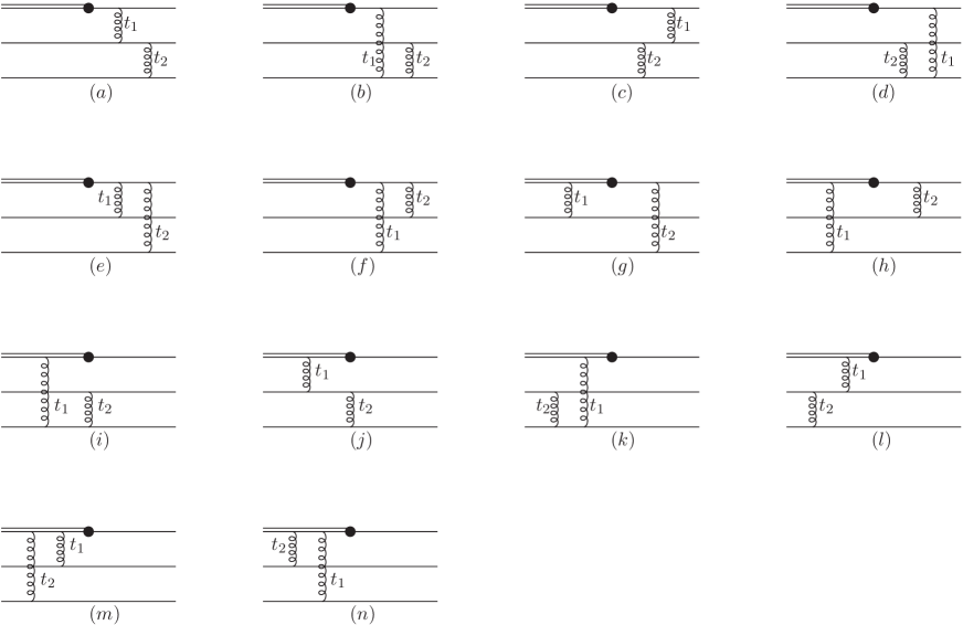
Figure 1: The lowest order diagrams for the $\Lambda_{b}\to\Lambda\gamma$ decay. The solid lines, double lines, wavy lines and the black blub vertex denote the light quarks, b quark, gluon and the electromagnetic penguin vertex, respectively. Diagrams with triple-gluon vertex do not contribute since their color factors are all zero in the present case.

Collecting all contributions in Fig.1 and multiplying the corresponding Wilson coefficients, one then obtains a hard scattering amplitude $H_{l,\mu}^{\alpha^{\prime}\beta^{\prime}\gamma^{\prime}\alpha\beta\gamma}(x,x^{\prime},b,b^{\prime},M_{\Lambda_{b}})=\sum_{i}C_{l}^{eff}(t)\tilde{H}_{l,\mu}^{i,\alpha^{\prime}\beta^{\prime}\gamma^{\prime}\alpha\beta\gamma}(x,x^{\prime},b,b^{\prime},M_{\Lambda_{b}})$. Here we have labelled the hard scale as $t$ which is taken to be the larger of the two variables $t_{1,2}$ associated with the virtual gluon momentum in Fig. 1, i.e. $t=\textrm{max}(t_{1}^{i},t_{2}^{i})$. The expressions for $t_{1,2}$ are listed in Appendix C.

Finally a RG running is applied to the hard scattering amplitude to match the scale $\nu$ in the wave functions and we obtainLip

$$H_{l,\mu}^{\alpha^{\prime}\beta^{\prime}\gamma^{\prime}\alpha\beta\gamma}(x,x^{\prime},b,b^{\prime},M_{\Lambda_{b}},\nu)=$$

$$\textrm{exp}[-6\int_{\nu}^{t}\frac{d\overline{\mu}}{\overline{\mu}}\gamma_{q}(\alpha_{s}(\overline{\mu}))]\times H_{l,\mu}^{\alpha^{\prime}\beta^{\prime}\gamma^{\prime}\alpha\beta\gamma}(x,x^{\prime},b,b^{\prime},M_{\Lambda_{b}})$$ (12)

The form factors are obtained by grouping relevant terms according to the definition in eq. (3). Using eq.(10) we obtain a generic expression for the form factors corresponding to each diagram as

$$F^{i}_{l} = \sum_{j=V,A,T}\frac{\pi^{2}}{27}f^{j}_{\Lambda}f_{{}_{\Lambda_{b}}}\int[Dx]\int[Db]^{i}C_{l}^{eff}(t^{i})$$

$$\Psi_{\Lambda_{b}}(x)\Phi_{\Lambda}^{j}(x^{\prime})\textrm{exp}[-S^{i}]H_{F}^{ij}\Omega^{i}$$

$$S = \sum^{3}_{k=2}s(\omega,x_{k}p^{-})+\sum^{3}_{k=1}s(\omega^{\prime},x_{k}^{\prime}p^{\prime+})+3\int_{\omega}^{t}\frac{d\overline{\mu}}{\overline{\mu}}\gamma_{q}(\alpha_{s}(\overline{\mu}))+3\int_{\omega^{\prime}}^{t}\frac{d\overline{\mu}}{\overline{\mu}}\gamma_{q}(\alpha_{s}(\overline{\mu}))$$ (13)

where $F^{i}_{l}$ represents the form factors contributed by the “i” the diagram in which operators with the Wilson coefficients $C_{l}^{eff}$ are inserted, in our case $C_{l}^{eff}=C_{7}^{eff}$. The superscript $j$ labels $V,A$, and $T$ related to the spin structure of the valence quarks in the $\Lambda$ baryon with $f^{A}_{\Lambda}=f^{V}_{\Lambda}=f_{\Lambda}$. The explicit expressions of $\Omega^{i}$ are presented in Appendix D. The functions $H_{F}^{ij}$ are given in Appendix E. The total form factors are obtained by summing over contributions from all diagrams.

III Numerical results

We are now ready to evaluate the form factors numerically. For concreteness, we adopt the model proposed in Ref.lambdabwave for the $\Lambda_{b}$ baryon distribution amplitude $\Psi$,

$$\Psi(x_{1},x_{2},x_{3})=Nx_{1}x_{2}x_{3}\mathrm{exp}[-{M^{2}_{\Lambda_{b}}\over 2\beta^{2}x_{1}}-{m^{2}_{q}\over 2\beta^{2}x_{2}}-{m^{2}_{q}\over 2\beta^{2}x_{3}}].$$ (14)

The normalization constant $N$ is obtained by the condition:

$$\int[dx]\Psi(x_{1},x_{2},x_{3})=1.$$ (15)

The decay constant $f_{\Lambda_{b}}$ is determined by fitting $B(\Lambda_{b}\to\Lambda_{c}l\overline{\nu})$ whose central value is 5% measured by DELPHIexpLic using the same PQCD method. When fitting the data we truncate the double log Sudakov factor in such a way that the factor exp(-s) is smaller than 1 following the prescription in Ref.suda1 . Our numbers for $f_{\Lambda_{b}}$ are different from those obtained in Ref.Lic where a $B(\Lambda_{b}\to\Lambda_{c}l\overline{\nu})$ was taken to be 2%. We also have chosen cut-offs as $\omega=1.14min(1/\tilde{b}_{1},1/\tilde{b}_{2},1/\tilde{b}_{3})$ and $\omega^{\prime}=1.14min(1/\tilde{b}^{\prime}_{1},1/\tilde{b}^{\prime}_{2},1/\tilde{b}^{\prime}_{3})$. The factor 1.14 is adopted because this cut-off choice can result in form factors which vary smoothly with square of momentum transfer in fitting $\Lambda_{b}\to\Lambda_{c}l\overline{\nu}$ process and it reflects the resummation of next-to-leading double log in higher order radiative correctionsLip2 . Also the $\beta$ and $m_{q}$ in the heavy baryon wavefunction distribution need to be fixed. In Ref.Lic ; Lip ; LiJ , $\beta=1$ GeV and $m_{q}=0.3$ GeV were used to estimate $\Lambda_{b}\to\Lambda_{c}l\bar{\nu}$, $\Lambda_{b}\to pl\bar{\nu}$ and also $\Lambda_{b}\to\Lambda J/\psi$ decay rates. $\beta$ should not be too much smaller than 1 GeV if the form factors are dominated by perturbative contributions. Therefore we will let both $\beta$ and $m_{q}$ vary within ranges as $0.6\sim 1$GeV and $0.2\sim 0.3$GeV. The results for $f_{\Lambda_{b}}$ are shown in Table 1 for different parameter choices respectively.

Table 1: Decay constant $f_{\Lambda_{b}}$ for different choices of $\beta$ and $m_{q}$, respectively.

$f_{\Lambda_{b}}$(GeV)	$\beta=0.6$GeV	$\beta=0.7$GeV	$\beta=0.8$GeV	$\beta=0.9$GeV	$\beta=1$GeV
$m_{q}=0.2$GeV	$0.691\times 10^{-3}$	$0.841\times 10^{-3}$	$1.02\times 10^{-3}$	$1.21\times 10^{-3}$	$1.43\times 10^{-3}$
$m_{q}=0.3$GeV	$1.27\times 10^{-3}$	$1.45\times 10^{-3}$	$1.65\times 10^{-3}$	$1.88\times 10^{-3}$	$2.12\times 10^{-3}$

The $\Lambda$ baryon distribution amplitudes have been studied using QCD sum rules. In this work, we adopt the model proposed in Ref.lambdawave ,

$$\phi^{V}(x_{1},x_{2},x_{3})=42\phi_{as}(x_{1},x_{2},x_{3})[0.18(x_{3}^{2}-x_{2}^{2})+0.10(x_{2}-x_{3})],$$

$$\phi^{A}(x_{1},x_{2},x_{3})=-42\phi_{as}(x_{1},x_{2},x_{3})[0.26(x_{3}^{2}+x_{2}^{2})+0.34x_{1}^{2}-0.56x_{2}x_{3}-0.24x_{1}(x_{2}+x_{3})],$$

$$\phi^{T}(x_{1},x_{2},x_{3})=42\phi_{as}(x_{1},x_{2},x_{3})[1.2(x_{2}^{2}-x_{3}^{2})-1.4(x_{2}-x_{3})],$$

$$\phi_{as}(x_{1},x_{2},x_{3})=120x_{1}x_{2}x_{3}.$$ (16)

The asymmetric distribution in the momentum fractions of the three quarks implies $SU(3)$ symmetry breaking.

The constants $f_{\Lambda}$ and $f_{\Lambda}^{T}$ are fixed to belambdawave

$$f_{\Lambda}=0.63\times 10^{-2}\mathrm{GeV}^{2},\;\;f_{\Lambda}^{T}=0.063\times 10^{-2}\mathrm{GeV}^{2}.$$ (17)

Finally to obtain the branching ratio for $\Lambda_{b}\to\Lambda\gamma$, for definitiveness we fix rest of the parameters as following. The parameter $\Lambda_{QCD}$ which enters in the strong coupling constant and various Wilson coefficients, the b quark mass and the CKM mixing parameters are set to be: $\Lambda_{QCD}$ at 0.2 GeV, $m_{b}=4.8$ GeV, and the CKM mixing parameters are set to their central valuesdata0 : $s_{12}=0.2243$, $s_{23}=0.00413$, $s_{13}=0.0037$ and $\delta_{13}=1.05$.

Our explicit calculations show that $F_{L}=0$ and a non-zero value for $F_{R}$ as expected since light quark and light baryon masses have been neglected. The contributions from each diagrams for $F_{R}$ are shown in Appendix E. The resulting branching ratio is shown in Table 2. We see that the branching ratio for $\Lambda_{b}\to\Lambda\gamma$ is in the range of $(4.3\sim 6.8)\times 10^{-8}$.

Table 2: Branching ratio(BR) of $\Lambda_{b}\to\Lambda\gamma$ for different choices of $\beta$ and $m_{q}$ with Sudakov truncation.

BR$(\times 10^{8})$	$\beta=0.6$GeV	$\beta=0.7$GeV	$\beta=0.8$GeV	$\beta=0.9$GeV	$\beta=1$GeV
$m_{q}=0.2$GeV	$6.76$	$6.26$	$6.19$	$4.90$	$4.67$
$m_{q}=0.3$GeV	$6.42$	$5.75$	$5.61$	$4.44$	$4.32$

IV Discussions and conclusions

In this work we have used the perturbative QCD approach to evaluate the branching ratio for radiative decay $\Lambda_{b}\rightarrow\Lambda\gamma$. This process occurs via penguin diagrams. Our results are shown in Table 2. The branching ratio obtained is much smaller than results obtained, shown in Table 3, using other methods.

Table 3: Decay branching ratios (B) of $\Lambda_{b}\to\Lambda\gamma$ based on the form factors from the QCD sum rule approach, the covariant oscillator quark model, HQET and MIT bag model, respectively

Model	pole modelMannel	QCD sum ruleHuang	covariant oscillator quark modelMohanta	HQETCheng	bag modelCheng
B	$(0.10\sim 0.45)\times 10^{-5}$	$(3.7\pm 0.5)\times 10^{-5}$	$0.23\times 10^{-5}$	$(1.2\sim 1.9)\times 10^{-5}$	$0.6\times 10^{-5}$

There are uncertainties in PQCD predictions due to unknown parameters in wavefunctions. We have tried to understand such uncertainties by varying several relevant parameters. Within reasonable ranges of the parameters it is not possible to obtain a branching ratio larger than $10^{-7}$. We have considered another possible uncertainty in the method used here. This is the choice of the infrared cut-offs $\omega(\omega^{\prime})$ in the Sudakov suppression factor which damps the perturbative contributions. In our calculations the cut-offs are set to the conventional values with $\omega=1.14min(1/\tilde{b}_{1},1/\tilde{b}_{2},1/\tilde{b}_{3})$ and $\omega^{\prime}=1.14min(1/\tilde{b}^{\prime}_{1},1/\tilde{b}^{\prime}_{2},1/\tilde{b}^{\prime}_{3})$ discussed in the text. The factor 1.14 is adopted because this choice for cut-offs’ can result in form factors which vary smoothly with square of momentum transfer in fitting $\Lambda_{b}\to\Lambda_{c}l\overline{\nu}$ process and it reflects the resummation of next-to-leading double log in higher order radiative correctionsLip2 . We have checked with slightly different cut-offs and find impossible to obtain branching ratio to be as large as what listed in Table 3.

The prescription of truncating the factor exp(-s) to be smaller than 1 described in Ref.suda1 may also be a source for uncertainties. We therefore have evaluated the branching ratio without this truncation. The results are shown in Table 4. We see that the results are similar to those obtained in Table 2.

Table 4: Branching ratio(BR) of $\Lambda_{b}\to\Lambda\gamma$ for different choices of $\beta$ and $m_{q}$ without Sudakov truncation.

BR$(\times 10^{8})$	$\beta=0.6$GeV	$\beta=0.7$GeV	$\beta=0.8$GeV	$\beta=0.9$GeV	$\beta=1$GeV
$m_{q}=0.2$GeV	$8.60$	$7.22$	$5.91$	$4.92$	$4.60$
$m_{q}=0.3$GeV	$5.96$	$5.73$	$5.70$	$4.67$	$4.30$

We therefore conclude that within the PQCD framework, the branching ratio for $\Lambda_{b}\to\Lambda\gamma$ is much smaller than other model calculations. This is somewhat surprising since PQCD calculation for the branching ratio of $B\to K^{(*)}\gamma$ obtains a value of order consistent to other model calculations and also agrees with experimental value of about $4\times 10^{-5}$newbgamma . There is a huge suppression for $\Lambda_{b}\to\Lambda\gamma$. At this moment there is no data available for $\Lambda_{b}\to\Lambda\gamma$ yet. One has to wait for future experimental data to tell us more. If a branching ratio above $10^{-7}$ is measured at some future facilities, such as LHCb, the PQCD method used here will certainly need to be modified.

On the theoretical side, one expects the branching ratio for $\Lambda_{b}\to\Lambda\gamma$ to be smaller than that of $B\to K^{(*)}\gamma$ due to several suppression factors such as an additional $\alpha_{s}^{2}$ and a large momentum squared $q^{2}$ suppression factor as one more hard gluon is exchanged between quarks. There is also an additional Sudakov suppression factor due to an additional spectator quark involved in the process as can be seen from eq.(13).

One might question the applicability of PQCD method for the process under consideration. One notes that in the PQCD approach, both gluons are hard ones which excludes the possibility of including contributions where two spectator quarks (not involved in the weak interaction vertex) form a collective object first due to soft gloun exchanges, i.e. the diquark, and then this object interacts with the other quark by exchanging a hard gluon. If this contribution turns out to be the dominant one, the branching ratio may be substantially larger. At present there is no solid theoretical method to treat this effect yet, we do not have a definitive answer about this. We, however, note that estimate for $\Lambda_{b}\to\Lambda J/\psi$ using the same method gives a reasonable range compared with dataLiJ . This can be taken as a support for the applicability of the method to $\Lambda_{b}$ decays. Our result for $B(\Lambda_{b}\to\Lambda\gamma)$ represents a reasonable estimate. The branching ratio for $\Lambda_{b}\to\Lambda\gamma$ is in the range of $(4.3\sim 8.6)\times 10^{-8}$ which is smaller than predictions using other methods listed in Table 3. We have to wait for future experiments to provide more information.

Acknowledgements:

This work is supported in part by NNSFC, NSC and NCTS. We would like to thank Hsiang-nan Li and Cai-Dian Lü for helpful discussions. We also thank H.n. Li for providing us with the program for numerical integration.

Appendix A: the $b$ measures
The ordinary b measure is defined as

$$[d\mathbf{b}]={d^{2}\mathbf{b}\over(2\pi)^{2}}$$ (18)

The explicit forms of $[D\mathbf{b}]^{i}$ for each diagram $i$ in Fig. 1 are given by

$$[D\mathbf{b}]^{(a)}=[d\mathbf{b}_{1}][d\mathbf{b}_{3}][d\mathbf{b}_{1}^{\prime}][d\mathbf{b}_{3}^{\prime}],\;\;[D\mathbf{b}]^{(b)}=[d\mathbf{b}_{1}][d\mathbf{b}_{2}][d\mathbf{b}_{1}^{\prime}][d\mathbf{b}_{2}^{\prime}],$$

$$[D\mathbf{b}]^{(c)}=[d\mathbf{b}_{1}][d\mathbf{b}_{3}][d\mathbf{b}_{1}^{\prime}][d\mathbf{b}_{3}^{\prime}],\;\;[D\mathbf{b}]^{(d)}=[d\mathbf{b}_{1}][d\mathbf{b}_{2}][d\mathbf{b}_{1}^{\prime}][d\mathbf{b}_{2}^{\prime}],$$

$$[D\mathbf{b}]^{(e)}=[d\mathbf{b}_{2}][d\mathbf{b}_{2}^{\prime}][d\mathbf{b}_{3}^{\prime}],\;\;\;\;\;\;\;\;\;\;[D\mathbf{b}]^{(f)}=[d\mathbf{b}_{3}][d\mathbf{b}_{2}^{\prime}][d\mathbf{b}_{3}^{\prime}],$$

$$[D\mathbf{b}]^{(g)}=[d\mathbf{b}_{2}][d\mathbf{b}_{3}][d\mathbf{b}_{3}^{\prime}],\;\;\;\;\;\;\;\;\;\;[D\mathbf{b}]^{(h)}=[d\mathbf{b}_{2}][d\mathbf{b}_{3}][d\mathbf{b}_{2}^{\prime}]$$

$$[D\mathbf{b}]^{(i)}=[d\mathbf{b}_{1}][d\mathbf{b}_{2}][d\mathbf{b}_{1}^{\prime}][d\mathbf{b}_{2}^{\prime}],\;\;[D\mathbf{b}]^{(j)}=[d\mathbf{b}_{1}][d\mathbf{b}_{3}][d\mathbf{b}_{1}^{\prime}][d\mathbf{b}_{3}^{\prime}],$$

$$[D\mathbf{b}]^{(k)}=[d\mathbf{b}_{1}][d\mathbf{b}_{2}][d\mathbf{b}_{1}^{\prime}][d\mathbf{b}_{2}^{\prime}],\;\;[D\mathbf{b}]^{(l)}=[d\mathbf{b}_{1}][d\mathbf{b}_{3}][d\mathbf{b}_{1}^{\prime}][d\mathbf{b}_{3}^{\prime}],$$

$$[D\mathbf{b}]^{(m)}=[d\mathbf{b}_{2}][d\mathbf{b}_{3}][d\mathbf{b}_{2}^{\prime}],\;\;\;\;\;\;\;\;\;[D\mathbf{b}]^{(n)}=[d\mathbf{b}_{2}][d\mathbf{b}_{3}][d\mathbf{b}_{3}^{\prime}].$$ (19)

Appendix B: Hard scattering amplitudes $H_{l,\mu}^{i,\alpha^{\prime}\beta^{\prime}\gamma^{\prime}\alpha\beta\gamma}(x_{i},x_{i}^{\prime},\textbf{k}_{T},\textbf{k}_{T}^{\prime},M_{\Lambda_{b}})$

Expressions of amplitude $H_{l,\mu}^{i,\alpha^{\prime}\beta^{\prime}\gamma^{\prime}\alpha\beta\gamma}(x_{i},x_{i}^{\prime},\textbf{k}_{T},\textbf{k}_{T}^{\prime},M_{\Lambda_{b}})$ for each diagram in Fig. 1. In the following $O^{l}_{\mu}$ comes from the $\gamma$-matrix in the effective Hamiltonian, $O^{l=7}_{\mu}=\sigma_{\mu\nu}q^{\nu}R$

For the hard amplitude of Fig.1(a):

$$H_{\mu}^{a,\alpha^{\prime}\beta^{\prime}\gamma^{\prime}\alpha\beta\gamma}(x_{i},x_{i}^{\prime},\textbf{k}_{T},\textbf{k}_{T}^{\prime},M_{\Lambda_{b}})=$$

$$[\varepsilon^{abc}\varepsilon^{a^{\prime}b^{\prime}c^{\prime}}(T^{j})_{c^{\prime}c}(T^{j}T^{i})_{b^{\prime}b}(T^{i})_{a^{\prime}a}]g_{s}^{4}{(\gamma_{\rho})_{\gamma^{\prime}\gamma}[\gamma^{\rho}(\hbox to0.0pt{/\hss}p^{\prime}-\hbox to0.0pt{/\hss}k^{\prime}_{1}-\hbox to0.0pt{/\hss}k_{3})\gamma^{\lambda}]_{\beta^{\prime}\beta}[\gamma_{\lambda}(\hbox to0.0pt{/\hss}p^{\prime}-\hbox to0.0pt{/\hss}p+\hbox to0.0pt{/\hss}k_{1})O_{\mu}]_{\alpha^{\prime}\alpha}\over(p^{\prime}-k_{1}^{\prime}-k_{3})^{2}(p^{\prime}-p+k_{1})^{2}(p-p^{\prime}+k_{1}^{\prime}-k_{1})^{2}(k_{3}-k_{3}^{\prime})^{2}}$$

$$=C_{N}g_{s}^{4}{(\gamma_{\rho})_{\gamma^{\prime}\gamma}[\gamma^{\rho}(\hbox to0.0pt{/\hss}p^{\prime}-\hbox to0.0pt{/\hss}k^{\prime}_{1}-\hbox to0.0pt{/\hss}k_{3})\gamma^{\lambda}]_{\beta^{\prime}\beta}[\gamma_{\lambda}(\hbox to0.0pt{/\hss}p^{\prime}-\hbox to0.0pt{/\hss}p+\hbox to0.0pt{/\hss}k_{1})O_{\mu}]_{\alpha^{\prime}\alpha}\over[A_{a}+(\textbf{k}_{1T}^{\prime}+\textbf{k}_{3T})^{2}][B_{a}+\textbf{k}_{1T}^{2}][C_{a}+(\textbf{k}_{1T}-\textbf{k}_{1T}^{\prime})^{2}][D_{a}+(\textbf{k}_{3T}-\textbf{k}_{3T}^{\prime})^{2}]}$$ (20)

with

$$A_{a}=x_{3}(1-x_{1}^{\prime})\rho M_{\Lambda_{b}}^{2},B_{a}=(1-x_{1})\rho M_{\Lambda_{b}}^{2},C_{a}=(1-x_{1})(1-x_{1}^{\prime})\rho M_{\Lambda_{b}}^{2},D_{a}=x_{3}x_{3}^{\prime}\rho M_{\Lambda_{b}}^{2}$$ (21)

and the color factor

$$C_{N}=\varepsilon^{abc}\varepsilon^{a^{\prime}b^{\prime}c^{\prime}}(T^{j})_{c^{\prime}c}(T^{j}T^{i})_{b^{\prime}b}(T^{i})_{a^{\prime}a}={(N^{2}-1)(N+1)\over 12}$$ (22)

For the hard amplitude of Fig.1(b):

$$H_{\mu}^{b,\alpha^{\prime}\beta^{\prime}\gamma^{\prime}\alpha\beta\gamma}(x_{i},x_{i}^{\prime},\textbf{k}_{T},\textbf{k}_{T}^{\prime},M_{\Lambda_{b}})=$$

$$[\varepsilon^{abc}\varepsilon^{a^{\prime}b^{\prime}c^{\prime}}(T^{i}T^{j})_{c^{\prime}c}(T^{i})_{b^{\prime}b}(T^{j})_{a^{\prime}a}]g_{s}^{4}{(\gamma^{\rho})_{\beta^{\prime}\beta}[\gamma_{\rho}(\hbox to0.0pt{/\hss}p^{\prime}-\hbox to0.0pt{/\hss}k_{1}^{\prime}-\hbox to0.0pt{/\hss}k_{2})\gamma_{\lambda}]_{\gamma^{\prime}\gamma}[\gamma^{\lambda}(\hbox to0.0pt{/\hss}p^{\prime}-\hbox to0.0pt{/\hss}p+\hbox to0.0pt{/\hss}k_{1})O_{\mu}]_{\alpha^{\prime}\alpha}\over(p^{\prime}-k_{1}^{\prime}-k_{2})^{2}(p^{\prime}-p+k_{1})^{2}(p-p^{\prime}-k_{1}+k_{1}^{\prime})^{2}(k_{2}^{\prime}-k_{2})^{2}}$$

$$=C_{N}g_{s}^{4}{(\gamma^{\rho})_{\beta^{\prime}\beta}[\gamma_{\rho}(\hbox to0.0pt{/\hss}p^{\prime}-\hbox to0.0pt{/\hss}k_{1}^{\prime}-\hbox to0.0pt{/\hss}k_{2})\gamma_{\lambda}]_{\gamma^{\prime}\gamma}[\gamma^{\lambda}(\hbox to0.0pt{/\hss}p^{\prime}-\hbox to0.0pt{/\hss}p+\hbox to0.0pt{/\hss}k_{1})O_{\mu}]_{\alpha^{\prime}\alpha}\over[A_{b}+(\textbf{k}_{1T}^{\prime}+\textbf{k}_{2T})^{2}][B_{b}+\textbf{k}_{1T}^{2}][C_{b}+(\textbf{k}_{1T}-\textbf{k}_{1T}^{\prime})^{2}][D_{b}+(\textbf{k}_{2T}-\textbf{k}_{2T}^{\prime})^{2}]}$$ (23)

with

$$A_{b}=x_{2}(1-x_{1}^{\prime})\rho M_{\Lambda_{b}}^{2},B_{b}=(1-x_{1})\rho M_{\Lambda_{b}}^{2},C_{b}=(1-x_{1})(1-x_{1}^{\prime})\rho M_{\Lambda_{b}}^{2},D_{b}=x_{2}x_{2}^{\prime}\rho M_{\Lambda_{b}}^{2}$$ (24)

Inspection of the above calculations, one notices that one can easily obtain $H_{\mu}^{b,\alpha^{\prime}\beta^{\prime}\gamma^{\prime}\alpha\beta\gamma}(x_{i},x_{i}^{\prime},\textbf{k}_{T},\textbf{k}_{T}^{\prime},M_{\Lambda_{b}})$ from $H_{\mu}^{a,\alpha^{\prime}\beta^{\prime}\gamma^{\prime}\alpha\beta\gamma}(x_{i},x_{i}^{\prime},\textbf{k}_{T},\textbf{k}_{T}^{\prime},M_{\Lambda_{b}})$ and vice versa by simply exchanging the momentum indices 2 and 3 for k and $\textbf{k}^{\prime}$, and exchanging the positions of the Dirac indices $\gamma^{\prime}\gamma$ and $\beta^{\prime}\beta$. Due to these properties, the contributions to the form factors from the above two diagrams are the same. This fact can be easily understood by noticing the following properties of the quantities related to the distribution amplitudes: i) The distribution amplitudes $\Psi(x_{1},x_{2},x_{3})$, and $\phi^{A}(x_{1},x_{2},x_{3})$ are symmetric in exchanging $x_{2}$ and $x_{3}$, while $\phi^{V,T}(x_{1},x_{2},x_{3})$ are anti-symmetric in exchanging $x_{2}$ and $x_{3}$, as can be seen from eqs.(14) and (16). And ii) When exchanging the Dirac indices $\beta$ and $\gamma$, the expressions for $(Y_{\Lambda_{b}})_{\alpha\beta\gamma}(k_{i}\nu)$ in eq.(6), and terms proportional to $\phi^{A}$ for $(Y_{\Lambda})_{\alpha\beta\gamma}(k^{\prime}_{i},\nu)$ in eq.(7) will have a sign change, while terms proportional to $\phi^{V,T}$ remain the same. Since going from the contribution of diagram (a) to diagram (b) involves both actions: exchanging the momentum indices 2 and 3, and the Dirac indices $\beta$ and $\gamma$, this results in no sign changes for all the terms involved. After integrating out $x(x^{\prime})_{2,3}$ and $b(b^{\prime})_{2,3}$ to obtain the final form factors using eq.(13), one then obtains the same results for both diagrams (a) and (b).

Similar situation happens for the following pairs of diagrams: (c) and (d), (e) and (f), (g) and (h), (i) and (j), (k) and (l), and, (m) and (n). In the following we will only display the results for diagrams (a), (c), (e), (g), (i), (k) and (m). The expressions for diagrams (b), (d), (f), (h), (j), (l) and (n) can be obtained by exchanging $x(x^{\prime})_{2}$ and $x(x^{\prime})_{3}$, and also $\gamma^{\prime}\gamma$ and $\beta^{\prime}\beta$.

For the hard amplitude of Fig.1(c):

$$H_{\mu}^{c,\alpha^{\prime}\beta^{\prime}\gamma^{\prime}\alpha\beta\gamma}(x_{i},x_{i}^{\prime},\textbf{k}_{T},\textbf{k}_{T}^{\prime},M_{\Lambda_{b}})=$$

$$[\varepsilon^{abc}\varepsilon^{a^{\prime}b^{\prime}c^{\prime}}(T^{j})_{c^{\prime}c}(T^{i}T^{j})_{b^{\prime}b}(T^{i})_{a^{\prime}a}]g_{s}^{4}{(\gamma_{\rho})_{\gamma^{\prime}\gamma}[\gamma^{\lambda}(\hbox to0.0pt{/\hss}p-\hbox to0.0pt{/\hss}k_{1}-\hbox to0.0pt{/\hss}k_{3}^{\prime})\gamma^{\rho}]_{\beta^{\prime}\beta}[\gamma_{\lambda}(\hbox to0.0pt{/\hss}p^{\prime}-\hbox to0.0pt{/\hss}p+\hbox to0.0pt{/\hss}k_{1})O_{\mu}]_{\alpha^{\prime}\alpha}\over(p-k_{1}-k_{3}^{\prime})^{2}(p^{\prime}-p+k_{1})^{2}(p-p^{\prime}+k_{1}^{\prime}-k_{1})^{2}(k_{3}-k_{3}^{\prime})^{2}}$$

$$=C_{N}g_{s}^{4}{(\gamma_{\rho})_{\gamma^{\prime}\gamma}[\gamma^{\lambda}(\hbox to0.0pt{/\hss}p-\hbox to0.0pt{/\hss}k_{1}-\hbox to0.0pt{/\hss}k_{3}^{\prime})\gamma^{\rho}]_{\beta^{\prime}\beta}[\gamma_{\lambda}(\hbox to0.0pt{/\hss}p^{\prime}-\hbox to0.0pt{/\hss}p+\hbox to0.0pt{/\hss}k_{1})O_{\mu}]_{\alpha^{\prime}\alpha}\over[A_{c}+(\textbf{k}_{1T}+\textbf{k}_{3T}^{\prime})^{2}][B_{c}+\textbf{k}_{1T}^{2}][C_{c}+(\textbf{k}_{3T}-\textbf{k}_{3T}^{\prime})^{2}][D_{c}+(\textbf{k}_{1T}-\textbf{k}_{1T}^{\prime})^{2}]}$$ (25)

with

$$A_{c}=x_{3}^{\prime}(1-x_{1})\rho M_{\Lambda_{b}}^{2},B_{c}=(1-x_{1})\rho M_{\Lambda_{b}}^{2},C_{c}=x_{3}x_{3}^{\prime}\rho M_{\Lambda_{b}}^{2},D_{c}=(1-x_{1})(1-x_{1}^{\prime})\rho M_{\Lambda_{b}}^{2}$$ (26)

For the hard amplitude of Fig.1(e):

$$H_{\mu}^{e,\alpha^{\prime}\beta^{\prime}\gamma^{\prime}\alpha\beta\gamma}(x_{i},x_{i}^{\prime},\textbf{k}_{T},\textbf{k}_{T}^{\prime},M_{\Lambda_{b}})=$$

$$[\varepsilon^{abc}\varepsilon^{a^{\prime}b^{\prime}c^{\prime}}(T^{i})_{c^{\prime}c}(T^{i}T^{j})_{b^{\prime}b}(T^{j})_{a^{\prime}a}]g_{s}^{4}{(\gamma_{\rho})_{\gamma^{\prime}\gamma}[\gamma^{\rho}(\hbox to0.0pt{/\hss}p^{\prime}-\hbox to0.0pt{/\hss}k_{2}^{\prime}-\hbox to0.0pt{/\hss}k_{3})\gamma^{\lambda}(\hbox to0.0pt{/\hss}p^{\prime}-\hbox to0.0pt{/\hss}p+\hbox to0.0pt{/\hss}k_{1})O_{\mu}]_{\alpha^{\prime}\alpha}(\gamma_{\lambda})_{\beta^{\prime}\beta}\over(p^{\prime}-k_{2}^{\prime}-k_{3})^{2}(p^{\prime}-p+k_{1})^{2}(k_{2}^{\prime}-k_{2})^{2}(k_{3}-k_{3}^{\prime})^{2}}$$

$$=C_{N}g_{s}^{4}{(\gamma_{\rho})_{\gamma^{\prime}\gamma}[\gamma^{\rho}(\hbox to0.0pt{/\hss}p^{\prime}-\hbox to0.0pt{/\hss}k_{2}^{\prime}-\hbox to0.0pt{/\hss}k_{3})\gamma^{\lambda}(\hbox to0.0pt{/\hss}p^{\prime}-\hbox to0.0pt{/\hss}p+\hbox to0.0pt{/\hss}k_{1})O_{\mu}]_{\alpha^{\prime}\alpha}(\gamma_{\lambda})_{\beta^{\prime}\beta}\over[A_{e}+(\textbf{k}_{2T}^{\prime}+\textbf{k}_{3T})^{2}][B_{e}+\textbf{k}_{1T}^{2}][C_{e}+(\textbf{k}_{2T}-\textbf{k}_{2T}^{\prime})^{2}][D_{e}+(\textbf{k}_{3T}-\textbf{k}_{3T}^{\prime})^{2}]}$$ (27)

with

$$A_{e}=x_{3}(1-x_{1}^{\prime})\rho M_{\Lambda_{b}}^{2},B_{e}=(1-x_{1})\rho M_{\Lambda_{b}}^{2},C_{e}=x_{2}x_{2}^{\prime}\rho M_{\Lambda_{b}}^{2},D_{e}=x_{3}x_{3}^{\prime}\rho M_{\Lambda_{b}}^{2}$$ (28)

For the hard amplitude of Fig.1(g):

$$H_{\mu}^{g,\alpha^{\prime}\beta^{\prime}\gamma^{\prime}\alpha\beta\gamma}(x_{i},x_{i}^{\prime},\textbf{k}_{T},\textbf{k}_{T}^{\prime},M_{\Lambda_{b}})=$$

$$[\varepsilon^{abc}\varepsilon^{a^{\prime}b^{\prime}c^{\prime}}(T^{i})_{c^{\prime}c}(T^{j})_{b^{\prime}b}(T^{i}T^{j})_{a^{\prime}a}]g_{s}^{4}{(\gamma_{\rho})_{\gamma^{\prime}\gamma}[\gamma^{\rho}(\hbox to0.0pt{/\hss}p^{\prime}-\hbox to0.0pt{/\hss}k_{2}^{\prime}-\hbox to0.0pt{/\hss}k_{3})O_{\mu}(\hbox to0.0pt{/\hss}p-\hbox to0.0pt{/\hss}k_{3}-\hbox to0.0pt{/\hss}k_{2}^{\prime}+m_{b})\gamma^{\lambda}]_{\alpha^{\prime}\alpha}(\gamma_{\lambda})_{\beta^{\prime}\beta}\over[(p-k_{3}-k_{2}^{\prime})^{2}-m_{b}^{2}](p^{\prime}-k_{2}^{\prime}-k_{3})^{2}(k_{2}^{\prime}-k_{2})^{2}(k_{3}^{\prime}-k_{3})^{2}}$$

$$=C_{N}g_{s}^{4}{(\gamma_{\rho})_{\gamma^{\prime}\gamma}[\gamma^{\rho}(\hbox to0.0pt{/\hss}p^{\prime}-\hbox to0.0pt{/\hss}k_{2}^{\prime}-\hbox to0.0pt{/\hss}k_{3})O_{\mu}(\hbox to0.0pt{/\hss}p-\hbox to0.0pt{/\hss}k_{3}-\hbox to0.0pt{/\hss}k_{2}^{\prime}+m_{b})\gamma^{\lambda}]_{\alpha^{\prime}\alpha}(\gamma_{\lambda})_{\beta^{\prime}\beta}\over[A_{g}+(\textbf{k}_{2T}^{\prime}+\textbf{k}_{3T})^{2}][B_{g}+(\textbf{k}_{2T}^{\prime}+\textbf{k}_{3T})^{2}][C_{g}+(\textbf{k}_{2T}-\textbf{k}_{2T}^{\prime})^{2}][D_{g}+(\textbf{k}_{3T}-\textbf{k}_{3T}^{\prime})^{2}]}$$ (29)

with

$$A_{g}=(x_{2}^{\prime}(1-x_{3})\rho+x_{3})M_{\Lambda_{b}}^{2},B_{g}=x_{3}(1-x_{2}^{\prime})\rho M_{\Lambda_{b}}^{2},C_{g}=x_{2}x_{2}^{\prime}\rho M_{\Lambda_{b}}^{2},D_{g}=x_{3}x_{3}^{\prime}\rho M_{\Lambda_{b}}^{2}$$ (30)

For the hard amplitude of Fig.1(i):

$$H_{\mu}^{i,\alpha^{\prime}\beta^{\prime}\gamma^{\prime}\alpha\beta\gamma}(x_{i},x_{i}^{\prime},\textbf{k}_{T},\textbf{k}_{T}^{\prime},M_{\Lambda_{b}})=$$

$$[\varepsilon^{abc}\varepsilon^{a^{\prime}b^{\prime}c^{\prime}}(T^{i}T^{j})_{c^{\prime}c}(T^{i})_{b^{\prime}b}(T^{j})_{a^{\prime}a}]g_{s}^{4}{[\gamma_{\rho}(\hbox to0.0pt{/\hss}p^{\prime}-\hbox to0.0pt{/\hss}k_{1}^{\prime}-\hbox to0.0pt{/\hss}k_{2})\gamma_{\lambda}]_{\gamma^{\prime}\gamma}[O_{\mu}(\hbox to0.0pt{/\hss}p-\hbox to0.0pt{/\hss}p^{\prime}-\hbox to0.0pt{/\hss}k_{1}^{\prime}+m_{b})\gamma^{\lambda}]_{\alpha^{\prime}\alpha}(\gamma^{\rho})_{\beta^{\prime}\beta}\over[(p-p^{\prime}+k_{1}^{\prime})^{2}-m_{b}^{2}](p^{\prime}-k_{1}^{\prime}-k_{2})^{2}(p-p^{\prime}-k_{1}+k_{1}^{\prime})^{2}(k_{2}^{\prime}-k_{2})^{2}}$$

$$=C_{N}g_{s}^{4}{[\gamma_{\rho}(\hbox to0.0pt{/\hss}p^{\prime}-\hbox to0.0pt{/\hss}k_{1}^{\prime}-\hbox to0.0pt{/\hss}k_{2})\gamma_{\lambda}]_{\gamma^{\prime}\gamma}[O_{\mu}(\hbox to0.0pt{/\hss}p-\hbox to0.0pt{/\hss}p^{\prime}-\hbox to0.0pt{/\hss}k_{1}^{\prime}+m_{b})\gamma^{\lambda}]_{\alpha^{\prime}\alpha}(\gamma^{\rho})_{\beta^{\prime}\beta}\over[A_{i}+(\textbf{k}_{2T}+\textbf{k}_{1T}^{\prime})^{2}][B_{i}+(\textbf{k}_{1T}^{\prime}+\textbf{k}_{2T})^{2}][C_{i}+(\textbf{k}_{1T}-\textbf{k}_{1T}^{\prime})^{2}][D_{i}+(\textbf{k}_{2T}-\textbf{k}_{2T}^{\prime})^{2}]}$$ (31)

with

$$A_{i}=(1-x_{1}^{\prime})\rho M_{\Lambda_{b}}^{2},B_{i}=x_{2}(1-x_{1}^{\prime})\rho M_{\Lambda_{b}}^{2},C_{i}=(1-x_{1})(1-x_{1}^{\prime})\rho M_{\Lambda_{b}}^{2},D_{i}=x_{2}x_{2}^{\prime}\rho M_{\Lambda_{b}}^{2}$$ (32)

For the hard amplitude of Fig.1(k):

$$H_{\mu}^{k,\alpha^{\prime}\beta^{\prime}\gamma^{\prime}\alpha\beta\gamma}(x_{i},x_{i}^{\prime},\textbf{k}_{T},\textbf{k}_{T}^{\prime},M_{\Lambda_{b}})=$$

$$[\varepsilon^{abc}\varepsilon^{a^{\prime}b^{\prime}c^{\prime}}(T^{i}T^{j})_{c^{\prime}c}(T^{j})_{b^{\prime}b}(T^{i})_{a^{\prime}a}]g_{s}^{4}{[\gamma_{\rho}(\hbox to0.0pt{/\hss}p-\hbox to0.0pt{/\hss}k_{1}-\hbox to0.0pt{/\hss}k_{2}^{\prime})\gamma_{\lambda}]_{\gamma^{\prime}\gamma}[O_{\mu}(\hbox to0.0pt{/\hss}p-\hbox to0.0pt{/\hss}p^{\prime}+\hbox to0.0pt{/\hss}k_{1}^{\prime}+m_{b})\gamma^{\rho}]_{\alpha^{\prime}\alpha}(\gamma^{\lambda})_{\beta^{\prime}\beta}\over[(p-p^{\prime}+k_{1}^{\prime})^{2}-m_{b}^{2}](p-k_{1}-k_{2}^{\prime})^{2}(p-p^{\prime}-k_{1}+k_{1}^{\prime})^{2}(k_{2}^{\prime}-k_{2})^{2}}$$

$$=C_{N}g_{s}^{4}{[\gamma_{\rho}(\hbox to0.0pt{/\hss}p-\hbox to0.0pt{/\hss}k_{1}-\hbox to0.0pt{/\hss}k_{2}^{\prime})\gamma_{\lambda}]_{\gamma^{\prime}\gamma}[O_{\mu}(\hbox to0.0pt{/\hss}p-\hbox to0.0pt{/\hss}p^{\prime}+\hbox to0.0pt{/\hss}k_{1}^{\prime}+m_{b})\gamma^{\rho}]_{\alpha^{\prime}\alpha}(\gamma^{\lambda})_{\beta^{\prime}\beta}\over[A_{k}+\textbf{k}_{1T}^{\prime 2}][B_{k}+(\textbf{k}_{1T}+\textbf{k}_{2T}^{\prime})^{2}][C_{k}+(\textbf{k}_{1T}-\textbf{k}_{1T}^{\prime})^{2}][D_{k}+(\textbf{k}_{2T}-\textbf{k}_{2T}^{\prime})^{2}]}$$ (33)

with

$$A_{k}=(1-x_{1}^{\prime})\rho M_{\Lambda_{b}}^{2},B_{k}=x_{2}^{\prime}(1-x_{1})\rho M_{\Lambda_{b}}^{2},C_{k}=(1-x_{1})(1-x_{1}^{\prime})\rho M_{\Lambda_{b}}^{2},D_{k}=x_{2}x_{2}^{\prime}\rho M_{\Lambda_{b}}^{2}$$ (34)

For the hard amplitude of Fig.1(m):

$$H_{\mu}^{m,\alpha^{\prime}\beta^{\prime}\gamma^{\prime}\alpha\beta\gamma}(x_{i},x_{i}^{\prime},\textbf{k}_{T},\textbf{k}_{T}^{\prime},M_{\Lambda_{b}})=$$

$$[\varepsilon^{abc}\varepsilon^{a^{\prime}b^{\prime}c^{\prime}}(T^{j})_{c^{\prime}c}(T^{i})_{b^{\prime}b}(T^{i}T^{j})_{a^{\prime}a}]g_{s}^{4}{(\gamma_{\lambda})_{\gamma^{\prime}\gamma}[O_{\mu}(\hbox to0.0pt{/\hss}p-\hbox to0.0pt{/\hss}p^{\prime}+\hbox to0.0pt{/\hss}k_{1}^{\prime}+m_{b})\gamma_{\rho}(\hbox to0.0pt{/\hss}p-\hbox to0.0pt{/\hss}k_{2}-\hbox to0.0pt{/\hss}k_{3}^{\prime}+m_{b})\gamma^{\lambda}]_{\alpha^{\prime}\alpha}(\gamma^{\rho})_{\beta^{\prime}\beta}\over[(p-p^{\prime}+k_{1}^{\prime})^{2}-m_{b}^{2}][(p-k_{2}-k_{3}^{\prime})^{2}-m_{b}^{2}](k_{2}^{\prime}-k_{2})^{2}(k_{3}^{\prime}-k_{3})^{2}}$$

$$=C_{N}g_{s}^{4}{(\gamma_{\lambda})_{\gamma^{\prime}\gamma}[O_{\mu}(\hbox to0.0pt{/\hss}p-\hbox to0.0pt{/\hss}p^{\prime}+\hbox to0.0pt{/\hss}k_{1}^{\prime}+m_{b})\gamma_{\rho}(\hbox to0.0pt{/\hss}p-\hbox to0.0pt{/\hss}k_{2}-\hbox to0.0pt{/\hss}k_{3}^{\prime}+m_{b})\gamma^{\lambda}]_{\alpha^{\prime}\alpha}(\gamma^{\rho})_{\beta^{\prime}\beta}\over[A_{m}+\textbf{k}_{1T}^{\prime 2}][B_{m}+(\textbf{k}_{2T}+\textbf{k}_{3T}^{\prime})^{2}][C_{m}+(\textbf{k}_{2T}-\textbf{k}_{2T}^{\prime})^{2}][D_{m}+(\textbf{k}_{3T}-\textbf{k}_{3T}^{\prime})^{2}]}$$ (35)

with

$$A_{m}=(1-x_{1}^{\prime})\rho M_{\Lambda_{b}}^{2},B_{m}=(x_{3}^{\prime}(1-x_{2})\rho+x_{2})M_{\Lambda_{b}}^{2},C_{m}=x_{2}x_{2}^{\prime}\rho M_{\Lambda_{b}}^{2},D_{m}=x_{3}x_{3}^{\prime}\rho M_{\Lambda_{b}}^{2}$$ (36)

The expressions for the hard scattering amplitude in $b$ and $b^{\prime}$ space are obtained by making a Fourier transformation on $k_{T}$ and $k^{\prime}_{T}$ space. In the following we given one example for Fig.1(a) as an illustration. We note that the $k_{T}$ and $k^{\prime}_{T}$ dependencies are all in the denominators in the above expressions, one then just needs to consider that part of the fourier transformation. For Fig.1(a), it is given by

$$\Omega^{(a)}(x_{i},x_{i}^{\prime},\textbf{k}_{T},\textbf{k}_{T}^{\prime},M_{\Lambda_{b}})={1\over[A_{a}+(\textbf{k}_{1T}^{\prime}+\textbf{k}_{3T})^{2}][B_{a}+\textbf{k}_{1T}^{2}][C_{a}+(\textbf{k}_{1T}-\textbf{k}_{1T}^{\prime})^{2}][D_{a}+(\textbf{k}_{3T}-\textbf{k}_{3T}^{\prime})^{2}]}.$$ (37)

The fourier transformed expression is then given by

$$\Omega^{(a)}(x_{i},x_{i}^{\prime},b_{i},b_{i}^{\prime},M_{\Lambda_{b}})=\int e^{-i(\textbf{k}_{1T}\cdot\textbf{b}_{1}+\textbf{k}_{1T}^{\prime}\cdot\textbf{b}_{1}^{\prime}+\textbf{k}_{3T}\cdot\textbf{b}_{3}+\textbf{k}_{3T}^{\prime}\cdot\textbf{b}_{3}^{\prime})}\Omega^{(a)}(x_{i},x_{i}^{\prime},\textbf{k}_{T},\textbf{k}_{T}^{\prime},M_{\Lambda_{b}})d^{2}\textbf{k}_{1T}d^{2}\textbf{k}_{1T}^{\prime}d^{2}\textbf{k}_{3T}d^{2}\textbf{k}_{3T}^{\prime}.$$ (38)

Defining $\textbf{k}_{AT}\equiv\textbf{k}_{1T}^{\prime}+\textbf{k}_{3T}$, $\textbf{k}_{BT}\equiv\textbf{k}_{1T}$, $\textbf{k}_{CT}\equiv\textbf{k}_{1T}-\textbf{k}_{1T}^{\prime}$, and $\textbf{k}_{DT}\equiv\textbf{k}_{3T}-\textbf{k}_{3T}^{\prime}$, we rewrite the transformation as

$$\Omega^{(a)}(x_{i},x_{i}^{\prime},b_{i},b_{i}^{\prime},M_{\Lambda_{b}})$$

$$=\int{e^{-i[\textbf{k}_{AT}\cdot(\textbf{b}_{3}+\textbf{b}_{3}^{\prime})+\textbf{k}_{BT}\cdot(\textbf{b}_{1}+\textbf{b}_{1}^{\prime}-\textbf{b}_{3}-\textbf{b}_{3}^{\prime})+\textbf{k}_{CT}\cdot(-\textbf{b}_{1}^{\prime}+\textbf{b}_{3}+\textbf{b}_{3}^{\prime})+\textbf{k}_{DT}\cdot(-\textbf{b}_{3}^{\prime})]}1\over(\textbf{k}_{AT}^{2}+A_{a})(\textbf{k}_{BT}^{2}+B_{a})(\textbf{k}_{CT}^{2}+C_{a})(\textbf{k}_{DT}^{2}+D_{a})}d^{2}\textbf{k}_{AT}d^{2}\textbf{k}_{BT}d^{2}\textbf{k}_{CT}d^{2}\textbf{k}_{DT}$$

$$=(2\pi)^{4}K_{0}(\sqrt{A_{a}}|b_{3}+b_{3}^{\prime}|)K_{0}(\sqrt{B_{a}}|b_{1}+b_{1}^{\prime}-b_{3}-b_{3}^{\prime}|)K_{0}(\sqrt{C_{a}}|b_{1}^{\prime}-b_{3}-b_{3}^{\prime}|)K_{0}(\sqrt{D_{a}}|b_{3}^{\prime}|),$$ (39)

In the above we have used

$$\int d^{2}k{e^{i\mathbf{k}\cdot\mathbf{b}}\over k^{2}+A}=2\pi K_{0}(\sqrt{A}|\mathbf{b}|),A>0.$$ (40)

One obtains the expression for $H_{\mu}^{a,\alpha^{\prime}\beta^{\prime}\gamma^{\prime}\alpha\beta\gamma}(x_{i},x_{i}^{\prime},b,b^{\prime},M_{\Lambda_{b}})$ as

$$H_{\mu}^{a,\alpha^{\prime}\beta^{\prime}\gamma^{\prime}\alpha\beta\gamma}(x_{i},x_{i}^{\prime},b,b^{\prime},M_{\Lambda_{b}})=C_{N}g_{s}^{4}{(\gamma_{\rho})_{\gamma^{\prime}\gamma}[\gamma^{\rho}(\hbox to0.0pt{/\hss}p^{\prime}-\hbox to0.0pt{/\hss}k^{\prime}_{1}-\hbox to0.0pt{/\hss}k_{3})\gamma^{\lambda}]_{\beta^{\prime}\beta}[\gamma_{\lambda}(\hbox to0.0pt{/\hss}p^{\prime}-\hbox to0.0pt{/\hss}p+\hbox to0.0pt{/\hss}k_{1})O_{\mu}]_{\alpha^{\prime}\alpha}\widetilde{\Omega^{(a)}}(x_{i},x_{i}^{\prime},b_{i},b_{i}^{\prime},M_{\Lambda_{b}})}.$$

In carrying out the fourier transformations for other diagrams, two other forms of functions will be encountered. We list them in the following

$$\int d^{2}k{e^{i\mathbf{k}\cdot\mathbf{b}}\over(k^{2}+A)(k^{2}+B)}=\pi\int^{1}_{0}dz{|\mathbf{b}|K_{1}(\sqrt{Z_{1}}|\mathbf{b}|)\over\sqrt{Z_{1}}},A,B>0,$$

$$\int d^{2}k_{1}d^{2}k_{2}{e^{i(\mathbf{k_{1}}\cdot\mathbf{b_{1}}+\mathbf{k_{2}}\cdot\mathbf{b_{2}})}\over(k_{1}^{2}+A)(k_{2}^{2}+B)[(k_{1}+k_{2})^{2}+C]}=\pi^{2}\int^{1}_{0}{dz_{1}dz_{2}\over z_{1}(1-z_{1})}{\sqrt{X_{2}}\over\sqrt{|Z_{2}|}}K_{1}(\sqrt{X_{2}Z_{2}}),$$ (42)

where $A>0$ and $B$, $C$ arbitrary. $K_{0}$ and $K_{1}$ are the modified Bessel functions of the second kind. And

$$Z_{1}=Az+B(1-z),$$

$$Z_{2}=A(1-z_{2})+{z_{2}\over z_{1}(1-z_{1})}[B(1-z_{1})+Cz_{1}],$$

$$X_{2}=(\mathbf{b}_{1}-z_{1}\mathbf{b}_{2})^{2}+{z_{1}(1-z_{1})\over z_{2}}\mathbf{b}_{2}^{2}$$ (43)

Appendix C: The maximum of $t_{1,2}$

The hard scales, the maximal of $t_{1}^{i}$ and $t_{2}^{i}$ for diagrams (a), (c), (e), (g), (i), (k), and (m) in Fig. 1. Exchanging $b(b^{\prime})_{2}$ and $b(b^{\prime})_{3}$, one obtains the expressions for diagrams (b), (d), (f), (h), (j), (l) and (n). The expressions of $C_{i},D_{i}$ are collected in Appendix B.

i	$t_{1}^{i}$	$t_{2}^{i}$
(a)	$\textrm{max}\{\sqrt{|C_{a}|},\frac{1}{|\mathbf{b}_{1}^{\prime}-\mathbf{b}_{3}-\mathbf{b}_{3}^{\prime}|},\omega,\omega^{\prime}\}$	$\textrm{max}\{\sqrt{|D_{a}|},\frac{1}{|\mathbf{b}_{3}^{\prime}|},\omega,\omega^{\prime}\}$
(c)	$\textrm{max}\{\sqrt{|C_{c}|},\frac{1}{|\mathbf{b}_{1}^{\prime}|},\omega,\omega^{\prime}\}$	$\textrm{max}\{\sqrt{|D_{c}|},\frac{1}{|\mathbf{b}_{3}|},\omega,\omega^{\prime}\}$
(e)	$\textrm{max}\{\sqrt{|C_{e}|},\frac{1}{|\mathbf{b}_{2}^{\prime}|},\omega,\omega^{\prime}\}$	$\textrm{max}\{\sqrt{|D_{e}|},\frac{1}{|\mathbf{b}_{3}^{\prime}|},\omega,\omega^{\prime}\}$
(g)	$\textrm{max}\{\sqrt{|C_{g}|},\frac{1}{|\mathbf{b}_{2}|},\omega,\omega^{\prime}\}$	$\textrm{max}\{\sqrt{|D_{g}|},\frac{1}{|\mathbf{b}_{3}^{\prime}|},\omega,\omega^{\prime}\}$
(i)	$\textrm{max}\{\sqrt{|C_{i}|},\frac{1}{|\mathbf{b}_{1}|},\omega,\omega^{\prime}\}$	$\textrm{max}\{\sqrt{|D_{i}|},\frac{1}{|\mathbf{b}_{2}^{\prime}|},\omega,\omega^{\prime}\}$
(k)	$\textrm{max}\{\sqrt{|C_{k}|},\frac{1}{|\mathbf{b}_{1}-\mathbf{b}_{2}-\mathbf{b}_{2}^{\prime}|},\omega,\omega^{\prime}\}$	$\textrm{max}\{\sqrt{|D_{k}|},\frac{1}{|\mathbf{b}_{2}|},\omega,\omega^{\prime}\}$
(m)	$\textrm{max}\{\sqrt{|C_{m}|},\frac{1}{|\mathbf{b}_{2}^{\prime}|},\omega,\omega^{\prime}\}$	$\textrm{max}\{\sqrt{|D_{m}|},\frac{1}{|\mathbf{b}_{3}|},\omega,\omega^{\prime}\}$

Appendix D: Expressions of $\Omega^{i}$
The expression of $\Omega^{i}$ for diagrams (a), (c), (e), (g), (i), (k), and (m) in Fig. 1. Exchanging $b(b^{\prime})_{2}$ and $b(b^{\prime})_{3}$, one obtains the expressions for diagrams (b), (d), (f), (h), (j), (l) and (n).

$$\Omega^{(a)}=(2\pi)^{4}K_{0}(\sqrt{A_{a}}|\mathbf{b}_{3}+\mathbf{b}_{3}^{\prime}|)K_{0}(\sqrt{B_{a}}|\mathbf{b}_{1}+\mathbf{b}_{1}^{\prime}-\mathbf{b}_{3}-\mathbf{b}_{3}^{\prime}|)K_{0}(\sqrt{C_{a}}|\mathbf{b}_{1}^{\prime}-\mathbf{b}_{3}-\mathbf{b}_{3}^{\prime}|)K_{0}(\sqrt{D_{a}}|\mathbf{b}_{3}^{\prime}|)$$

$$\Omega^{(c)}=(2\pi)^{4}K_{0}(\sqrt{A_{c}}|\mathbf{b}_{3}+\mathbf{b}_{3}^{\prime}|)K_{0}(\sqrt{B_{c}}|\mathbf{b}_{1}+\mathbf{b}_{1}^{\prime}+\mathbf{b}_{3}+\mathbf{b}_{3}^{\prime}|)K_{0}(\sqrt{C_{c}}|\mathbf{b}_{1}^{\prime}|)K_{0}(\sqrt{D_{c}}|\mathbf{b}_{3}|)$$

$$\Omega^{(e)}=8\pi^{5}\int^{1}_{0}dz_{1}dz_{2}{1\over z_{1}(1-z_{1})}{\sqrt{X_{2}^{e}}\over\sqrt{|Z_{2}^{e}|}}K_{1}(\sqrt{X_{2}^{e}Z_{2}^{e}})K_{0}(\sqrt{D_{e}}|\mathbf{b}_{3}^{\prime}|)$$

$$\Omega^{(g)}=16\pi^{5}\int^{1}_{0}dz{|\mathbf{b}_{3}+\mathbf{b}_{3}^{\prime}|K_{1}(\sqrt{Z_{1}^{g}}|\mathbf{b}_{3}+\mathbf{b}_{3}^{\prime}|)\over\sqrt{Z_{1}^{g}}}K_{0}(\sqrt{C_{g}}|\mathbf{b}_{2}|)K_{0}(\sqrt{D_{g}}|\mathbf{b}_{3}^{\prime}|)$$

$$\Omega^{(i)}=(2\pi)^{4}K_{0}(\sqrt{A_{i}}|\mathbf{b}_{1}+\mathbf{b}_{1}^{\prime}-\mathbf{b}_{2}-\mathbf{b}_{2}^{\prime}|)K_{0}(\sqrt{B_{i}}|\mathbf{b}_{2}+\mathbf{b}_{2}^{\prime}|)K_{0}(\sqrt{C_{i}}|\mathbf{b}_{1}|)K_{0}(\sqrt{D_{i}}|\mathbf{b}_{2}^{\prime}|)$$

$$\Omega^{(k)}=(2\pi)^{4}K_{0}(\sqrt{A_{k}}|\mathbf{b}_{1}+\mathbf{b}_{1}^{\prime}-\mathbf{b}_{2}-\mathbf{b}_{2}^{\prime}|)K_{0}(\sqrt{B_{k}}|\mathbf{b}_{2}+\mathbf{b}_{2}^{\prime}|)K_{0}(\sqrt{C_{k}}|\mathbf{b}_{1}-\mathbf{b}_{2}-\mathbf{b}_{2}^{\prime}|)K_{0}(\sqrt{D_{k}}|\mathbf{b}_{2}|)$$

$$\Omega^{(m)}=8\pi^{5}\int^{1}_{0}dz_{1}dz_{2}{1\over z_{1}(1-z_{1})}{\sqrt{X_{2}^{m}}\over\sqrt{|Z_{2}^{m}|}}K_{1}(\sqrt{X_{2}^{m}Z_{2}^{m}})K_{0}(\sqrt{D_{m}}|\mathbf{b}_{3}|)$$

with

$$X_{2}^{e}=(\mathbf{b}_{2}^{\prime}+z_{1}\mathbf{b}_{2})^{2}+{z_{1}(1-z_{1})\over z_{2}}\mathbf{b}_{2}^{2},Z_{2}^{e}=A_{e}(1-z_{2})+{z_{2}\over z_{1}(1-z_{1})}[B_{e}(1-z_{1})+C_{e}z_{1}]$$

$$Z_{1}^{g}=A_{g}z+B_{g}(1-z)$$

$$X_{2}^{m}=(\mathbf{b}_{2}^{\prime}+z_{1}\mathbf{b}_{2})^{2}+{z_{1}(1-z_{1})\over z_{2}}\mathbf{b}_{2}^{2},Z_{2}^{m}=A_{m}(1-z_{2})+{z_{2}\over z_{1}(1-z_{1})}[B_{m}(1-z_{1})+C_{m}z_{1}]$$

Appendix E: Expressions for $H_{F}^{ij}$

In this appendix we list $H^{ij}_{F}$ corresponding to the form factors defined in eq.(13). We use $\tilde{F}_{R}^{j}$ for each diagram. The expressions for diagrams (a), (e), (g), (i), (k), and (m) in Fig. 1, whenever non-zero, are listed in the following. The expressions for diagrams (b), (f), (h), (j), (l) and (n) can be obtained by exchanging $x(x^{\prime})_{2}$ and $x(x^{\prime})_{3}$ and changing the signs for expressions $F_{R}^{V,T}$. Diagrams (c) and (d) have no contributions to $\Lambda_{b}\to\Lambda\gamma$. $\tilde{F}_{L}$ is equal to zero in our approximation.

For the hard amplitudes of Fig.1(a):

$$\widetilde{F_{R}^{A}}=8x_{3}\rho^{2}M_{\Lambda_{b}}^{4}$$ (46)

The relation between the tilde form factors listed above and the form factors in eq.(3) is as the following, taking $\tilde{F}_{R}^{A}$ as an example, $F^{A}_{R}=\frac{\pi^{2}}{27}f^{j}_{\Lambda}f_{{}_{\Lambda_{b}}}\int[Dx]\int[Db]^{i}C_{l}^{eff}(t^{i})\Psi_{\Lambda_{b}}(x)\Phi_{\Lambda}^{j}(x^{\prime})\textrm{exp}[-S^{i}]\tilde{F}^{A}_{R}\Omega^{i}$. For this example $j=A$, and $f^{A}_{\Lambda}=f_{\Lambda}$. For Fig.1(a), ‘i’ takes the value ‘a’. Similar for other form factors and diagrams.

The other non-zero contributions are

$$Fig.1(e): \widetilde{F_{R}^{V}}=\widetilde{F_{R}^{A}}=-4M_{\Lambda_{b}}^{4}\rho^{2}x_{3},$$

$$Fig.1(g): \widetilde{F_{R}^{V}}=4M_{\Lambda_{b}}^{3}(m_{b}\rho+M_{\Lambda_{b}}(-2x_{3}(-1+\rho)+(1+x_{2}^{\prime}(-1+\rho))\rho))$$

$$\widetilde{F_{R}^{A}}=4M_{\Lambda_{b}}^{3}(-1+\rho)(m_{b}+M_{\Lambda_{b}}(-1+x_{2}^{\prime}\rho)),$$

$$Fig.1(i): \widetilde{F_{R}^{A}}=8M_{\Lambda_{b}}^{3}x_{2}(m_{b}(-1+\rho)+M_{\Lambda_{b}}(1+(-1+x_{1}^{\prime})\rho)),$$

$$Fig.1(k): \widetilde{F_{R}^{A}}=8M_{\Lambda_{b}}^{3}\rho x_{2}^{\prime}(m_{b}+M_{\Lambda_{b}}(-1+\rho)),$$

$$Fig.1(m): \widetilde{F_{R}^{V}}=-4M_{\Lambda_{b}}^{2}(-m_{b}^{2}(-2+\rho)+M_{\Lambda_{b}}m_{b}(x_{2}-x_{2}\rho+(-1+x_{1}^{\prime}+x_{3}^{\prime})\rho)$$ (47)

$$\;\;\;\;\;\;+M_{\Lambda_{b}}^{2}(-2+(2-x_{1}^{\prime}+x_{3}^{\prime})\rho-x_{3}^{\prime}\rho^{2}+x_{2}(1+(-1+x_{1}^{\prime})\rho)))$$

$$\widetilde{F_{R}^{A}}=-4M_{\Lambda_{b}}^{2}(m_{b}^{2}\rho+M_{\Lambda_{b}}m_{b}(-2+x_{2}(1+\rho)+(-1+x_{1}^{\prime}+x_{3}^{\prime})\rho)$$

$$\;\;\;\;\;\;+M_{\Lambda_{b}}^{2}(2-(2+x_{1}^{\prime}+x_{3}^{\prime})\rho+x_{3}^{\prime}\rho^{2}+x_{2}(-1+(1+x_{1}^{\prime})\rho)))$$

References

(1)CLEO Collaboration, M.S. Alam et al., Phys. Rev. Lett.
74 (1995) 2885.
(2)Belle Collaboration, P.
Koppenburg et al., Phys.Rev.Lett. 93 (2004) 061803, BABAR
Collaboration, B. Aubert et al., arXiv:hep-ex/0507001.
(3)Belle Collaboration, M. Nakao et al., Phys. Rev. D69 (2004) 112001 ;
BABAR Collaboration, B. Aubert et al., Phys. Rev. D70 (2004)
112006.
(4)S. Bertolini, F. Borzumati and A. Masiero, Phys. Rev. Lett.
59, (1987) 180; Mikolaj Misiak, Nucl.Phys. B393
(1993) 23; K. Adel, York-Peng Yao, Phys.Rev D49(1994) 4945;
Christoph Greub, Tobias Hurth, Daniel Wyler Phys.Rev D54
(1996) 3350; Nicolas Pott, Phys.Rev D54 (1996) 938; X.-G.
He, C.-S. Li and L.-L. Yang, Phys. Rev. D71 (2005) 054006;
Riccardo Barbieri, G.F. Giudice, Phys.Lett. B309 (1993) 86;
J.L. Hewett, Phys. Rev. Lett. 70 (1993) 1045; V. Barger,
M.S. Berger and R.J.N. Phillips, Phys. Rev. Lett. 70 (1993)
1368.
(5) N.G. Deshpande, P. Lo, J. Trampetic, G. Eilam and P. Singer,
Phys. Rev. Lett. 59 (1987) 183;
N.G. Deshpande, Josip Trampetic and Kuriakose Panose,
Phys.Lett.B214 (1988) 467; H.-N. Li and G.-L. Lin, Phys.
Rev. D60, (1999) 054001; M. Beneke, T. Feldmann and D.
Seidel, Nucl. Phys. B612 (2001) 25; S. W. Bosch and G.
Buchalla, Nucl. Phys. B621 (2002) 459; Ahmed Ali and A.Y.
Parkhomenko Eur.Phys.J C23 (2002) 89.
(6) M. Matsumori and A.I. Sanda, Y.-Y. Keum, Phys.
Rev. D72 (2005) 014013.
(7)M. Beneke, G. Buchalla, M. Neubert and
C.T. Sachrajda, Phys. Rev. Lett. 83 (1999) 1914; Nucl. Phys.
B591 (2000) 313; Nucl. Phys. B606 (2001) 245.
(8)Yong-Yeon Keum and Hsiang-nan Li, Phys. Rev. D63
(2001) 074006; Chuan-Hung Chen, Yong-Yeon Keum and Hsiang-nan Li,
Phys. Rev. D64 (2001) 112002; Yong-Yeon Keum, Hsiang-nan Li
and A.I. Sanda, Phys. Rev. D63 (2001) 054008; Chuan-Hung
Chen, Yong-Yeon Keum and Hsiang-nan Li, Phys. Rev. D66
(2002) 054013; Cai-Dian Lü, Kazumasa Ukai and Mao-Zhi Yang,
Phys. Rev. D63 (2001) 074009; Cai-Dian Lü and Mao-Zhi
Yang, Eur. Phys. J. C23 (2002) 275.
(9) C.-K. Chua, X.-G. He and W.-S. Hou, Phys. Rev. D60,
(1999) 014003.
(10)T. Mannel and S. Recksiegel, J. Phys. G24 (1998) 979.
(11)Chao-Shang Huang and Hua-Gang Yan, Phys. Rev. D59 (1999) 114022.
(12)R. Mohanta, A.K. Giri, M.P. Khanna, M. Ishida and S. Ishida, Prog. Theor. Phys. 102 (1999)
645.
(13)H.Y. Cheng, C-Y. Cheung, G-L. Lin, Y.C. Lin, T.-M.
Yan and H-L. Yu, Phys. Rev. D51 (1995) 1199.
(14)Hsien-Hung Shih, Shih-Chang Lee and Hsiang-nan Li, Phys. Rev. D59 (1999)
094014.
(15)Hsien-Hung Shih, Shih-Chang Lee and Hsiang-nan Li, Phys. Rev. D61 (2000)
114002.
(16)Chung-Hsien Chou, Hsien-Hung Shih, Shih-Chang Lee and Hsiang-nan Li, Phys. Rev. D65 (2002) 074030.