Radiative Corrections in K, D, and B decays

Abstract

In this talk I review recent developments in the calculation of radiative corrections to $K,D,B$ meson decays and discuss their impact on precision phenomenology.

I Motivation

The calculation of electromagnetic radiative corrections (RC) to a given observable is typically needed when the corresponding experimental measurement reaches the precision of a few percent. In the context of flavor physics, RC are truly at the basis for meaningful $\%$-level phenomenology for two-fold reasons:

• One one hand, RC are essential in extracting fundamental Standard Model parameters (like the CKM matrix elements) or weak hadronic matrix elements from precisely measured decay rates.

• On the other hand, recent experience shows that knowledge of radiative effects (such as emission of real photons) and their proper simulation are essential in performing precision measurements of branching fractions. In fact, real photon emission distorts the spectra of ”primary” decay products and thus affects the distribution of kinematic quantities used to select and count signal events RadCorr ; CGatti . The inclusion of RC in the experimental fits is known to produce shifts in the measured fractions at the several percent level.

The relevance of RC has been widely recognized in the K physics community, where high statistics experiments have triggered theoretical studies on the subject throughout the past decade. In heavy flavor physics this issue has received comparatively less attention. However, experiments at B and charm factories are approaching (in some channels) an accuracy level that requires a satisfactory understanding of radiative effects.

In this talk I review the theoretical framework for the study of RC to meson decays and describe recent theoretical efforts to obtain model-independent results despite the complications due to strong interactions.

II Radiative Corrections in Meson Decays: Overview

II.1 Theoretical Framework

Within the Standard Model (and its extensions) weak decays of mesons are studied via an effective lagrangian which factorizes the short- and long-distance physics:

$${\cal L}_{eff}=G_{F}\,\sum_{n}\ C_{n}\,O_{n}\ .$$ (1)

The Wilson coefficients $C_{n}$ encode information on short-distance degrees of freedom ($W$,$Z$,$t$ masses, for example), while the local dimension-six operators $O_{n}$ are constructed out of ”light” fields (quarks, leptons, gluons, photons).

In this framework, radiative corrections are accounted for by keeping track of $O(\alpha)$ effects in the calculation of both Wilson coefficients and hadronic matrix elements $\langle f|O_{n}|H\rangle$, eventually resulting in $O(\alpha)$ corrections to the decay rate $\Gamma(H\to f)$. The effective lagrangian framework leads to a natural separation into short- and long-distance corrections.
(i) Short distance (SD) corrections to the Wilson coefficients are calculated in perturbation theory and are by now well known for both semi-leptonic SDcorr1 and non-leptonic SDcorr2 operators. They typically result in large UV logs $\delta C_{n}\sim\alpha/\pi\log\left(M_{Z}/M_{H}\right)$, implying $\delta\Gamma_{\rm SD}/\Gamma\sim\,{\rm few}\,\%$.
(ii) Long distance (LD) corrections in general cannot be calculated in perturbation theory. The matrix elements $\langle f|O_{n}|H\rangle$ pose great challenges already without inclusion of $O(\alpha)$ effects, i.e. without virtual photons. Rigorous results can be obtained only in certain ranges of external momenta, corresponding to various hadronic Effective Field Theories (EFT), for example Chiral Perturbation Theory (ChPT), Heavy Quark Effective Theory (HQET), Heavy Hadron ChPT (HHChPT). In these cases it is possible to at least formally match from the quark-level to the hadronic EFT, thus generating $O(\alpha)$ effective hadronic vertices without introduction of large logarithms.

Despite the hadronic uncertainties, an important class of long distance corrections, the infrared (IR) effects, can be treated in a model-independent way. IR photons are defined as those with a wavelength much larger than the typical size of hadrons and therefore are not sensitive to the hadronic structure. Their effects can be calculated in the approximation of point-like hadrons, using only gauge invariance as the guiding principle in constructing the interaction lagrangian. The calculation of virtual photon corrections in the point-like approximation leads (as in standard QED) to IR divergent matrix elements and decay rates. One obtains IR-finite results only for the observable photon-inclusive decay rates such as

$$d\Gamma^{\rm incl}(E_{\gamma}^{\rm cut})=d\Gamma_{H\to f}+d\Gamma_{H\to f+\gamma}+d\Gamma_{H\to f+2\gamma}+\dots$$ (2)

with $\sum_{n}E_{\gamma}^{(n)}<E_{\gamma}^{\rm cut}$. The typical size of long-distance corrections is then given by $\delta\Gamma_{\rm LD}/\Gamma\sim\alpha/\pi\log\left(M_{H}/E_{\gamma}^{\rm cut}\right)$. When $E_{\gamma}^{\rm cut}\ll M_{H}$ the IR corrections are quite large and one needs to sum the effect to all orders in perturbation theory Weinberg:1965nx ; Yennie:1961ad .

II.2 General parameterization

Denoting with $\xi$ the collection of independent variables characterizing the non-radiative $H\to f$ decay and with $E_{\gamma}^{\rm cut}(\xi)$ the photon energy cut (in general $\xi$-dependent), the IR safe decay distribution can be written as follows

$$\frac{d\Gamma^{\rm incl}}{d\xi} = \left(\frac{\bar{E}}{M_{H}}\right)^{b(\xi)}\ \frac{d\Gamma^{(0)}}{d\xi}\,(1+\delta_{SD})$$ (3)

$$+ \delta_{LD}\left(\xi,E_{\gamma}^{\rm cut}(\xi)/\bar{E}\right)\ ,$$

where

$$b=-\frac{1}{8\pi^{2}}\sum_{m,n}\eta_{m}\eta_{n}e_{m}e_{n}\,\beta_{mn}^{-1}\ \log\frac{1+\beta_{mn}}{1-\beta_{mn}}~{}.$$ (4)

The sum in Eq. (4) runs over pairs of charged particles appearing in the initial and final states, $e_{m,n}$ are their electric charges, while $\eta_{m}=+1$ for out-going particles and $\eta_{m}=-1$ for in-going particles. $\beta_{mn}$ denotes the relative velocity of particles $m$ and $n$ in the rest frame of either of them Weinberg:1965nx :

$$\beta_{mn}=\left[1-\frac{m_{n}^{2}m_{m}^{2}}{(p_{n}\cdot p_{n})^{2}}\right]^{1/2}\ .$$ (5)

Eq. (3) requires some comments:

• $\bar{E}\ll M_{H}$ is an arbitrary soft scale, used to define IR photons . IR effects from real and virtual photons can be re-summed to all orders in perturbation theory Weinberg:1965nx and result in the overall factor $\left(\frac{\bar{E}}{M_{H}}\right)^{b(\xi)}$. This effect is model-independent and for $E_{\gamma}^{\rm cut}(\xi)\sim\bar{E}\ll M_{H}$ provides the largest long-distance correction.

• $\delta_{SD}$ is the model-independent short distance correction and always appears as a multiplicative correction to the ”Born” rate $\frac{d\Gamma^{(0)}}{d\xi}$.

• $\delta_{LD}\left(\xi,E_{\gamma}^{\rm cut}(\xi)/\bar{E}\right)$ is the long-distance, structure dependent correction. In general it does not factorize in the product of Born rate times a correction. In experimental setups where $E_{\gamma}^{\rm cut}(\xi)\sim E_{\gamma}^{\rm MAX}(\xi)\sim O(M_{H})$ , this is the dominant LD correction.

A parameterization similar to Eq. (3) is possible for the photon-energy distribution:

$$\frac{d\Gamma^{\rm incl}}{dE_{\gamma}\,d\xi}=\left(\frac{E_{\gamma}}{M_{H}}\right)^{b(\xi)}\,\frac{b(\xi)}{E_{\gamma}}\frac{d\Gamma^{(0)}}{d\xi}+\tilde{\delta}_{LD}\left(\xi,E_{\gamma}\right)\ .$$ (6)

The first term describes the universal soft-photon spectrum and is fixed by gauge invariance and kinematics. It is crucial in describing the soft radiative tails in experimental Monte Carlo studies CGatti . The second term starts at $O(E_{\gamma}^{0})$ and describes the hard-photon spectrum. The impact of $\tilde{\delta}_{LD}\left(\xi,E_{\gamma}\right)$ in simulations depends on the specific experimental setup.

In the parameterization of Eqs. (3) and (6) $\delta_{LD}$ and $\tilde{\delta}_{LD}$ are the quantities sensitive to the hadronic structure, and therefore the hardest to calculate. In Kaon decays, ChPT provides a universal tool to treat both virtual and real photon effects over all of the available phase space. The framework to treat both semileptonic  Knecht:1999ag and non-leptonic Ecker:2000zr decays has been fully developed and explicit calculation exist for $K\to\pi\pi$ k2pi , $K\to\pi\pi\pi$ k3pi , $K\to\pi\ell\nu$ radcorr1 ; radcorr1bis , $K\to\pi\pi\ell\nu$ kl4 . On the other hand, in most B (D) decays, rigorous EFT treatments only work in corners of phase space. In what follows I describe a few examples of calculations of radiative corrections to exclusive K, D, and B decays and their impact on phenomenology.

III Recent progress in exclusive modes

III.1 $K\to\pi\ell\bar{\nu}_{\ell}(\gamma)$ and $V_{us}$

	$\Delta^{K}_{SU(2)}$ (%)	$\Delta^{K\ell}_{\rm EM}(\%)$
		3-body              full
$K^{+}_{e3}$	2.31 $\pm$ 0.22   Gasser:1984ux ; radcorr1	-0.35 $\pm$ 0.16   radcorr1	-0.10 $\pm$ 0.16   radcorr1
$K^{0}_{e3}$	0	+0.30 $\pm$ 0.10   radcorr1bis	+0.55 $\pm$ 0.10   radcorr1bis
			+0.65 $\pm$ 0.15   radcorr2
$K^{+}_{\mu 3}$	2.31 $\pm$ 0.22   Gasser:1984ux ; radcorr1
$K^{0}_{\mu 3}$	0		+0.95 $\pm$ 0.15   radcorr2

Table 1: Summary of SU(2) and radiative correction factors for various $K_{\ell 3}$ decay modes. Refs. Gasser:1984ux ; radcorr1 ; radcorr1bis work within chiral perturbation theory to order $p^{4},e^{2}p^{2}$, while Ref. radcorr2 works within a hadronic model for Kaon electromagnetic interactions.

In this section I briefly review the extraction of $V_{us}$ from $K_{\ell 3}$ decays and the impact of radiative corrections. The decay rates for all $K_{\ell 3}$ modes ($K={K^{\pm},K^{0}},\ell=\mu,e$) can be written compactly as follows:

$$\Gamma(K_{\ell 3[\gamma]}) = \frac{G_{F}^{2}\,S_{\rm ew}\,M_{K}^{5}}{128\pi^{3}}\,C^{K}I^{K\ell}(\lambda_{i})\times$$

$$|V_{us} \times f_{+}^{K^{0}\pi^{-}}(0)|^{2}\times\Big{[}1+2\,\Delta^{K}_{SU(2)}+2\,\Delta^{K\ell}_{\rm EM}\Big{]}\ .$$

Here $G_{F}$ is the Fermi constant as extracted from muon decay, $S_{\rm ew}=1+\frac{2\alpha}{\pi}\left(1-\frac{\alpha_{s}}{4\pi}\right)\times\log\frac{M_{Z}}{M_{\rho}}+O(\frac{\alpha\alpha_{s}}{\pi^{2}})$ represents the short distance electroweak correction to semileptonic charged-current processes SDcorr1 , $C^{K}$ is a Clebsh-Gordan coefficient equal to 1 (1/$\sqrt{2}$) for neutral (charged) kaon decay, while $I^{K\ell}(\lambda_{i})$ is a phase-space integral depending on slope and curvature of the form factors. The latter are defined by the QCD matrix elements

$$\langle\pi^{j}(p_{\pi})|\bar{s}\gamma_{\mu}u|K^{i}(p_{K})\rangle=$$

$$f_{+}^{K^{i}\pi^{j}}(t)\,(p_{K}+p_{\pi})_{\mu}+f_{-}^{K^{i}\pi^{j}}(t)\,(p_{K}-p_{\pi})_{\mu}~{}.$$ (8)

As shown explicitly in Eq. (LABEL:eq:masterkl3), it is convenient to normalize the form factors of all channels to $f_{+}^{K^{0}\pi^{-}}(0)$, which in the following will simply be denoted by $f_{+}(0)$. The channel-dependent terms $\Delta^{K}_{SU(2)}$ and $\Delta^{K\ell}_{\rm EM}$ represent the isospin-breaking and long-distance electromagnetic corrections, respectively. A determination of $V_{us}$ from $K_{\ell 3}$ decays at the $1\%$ level requires $\sim 1\%$ theoretical control on $f_{+}(0)$ as well as the inclusion of $\Delta^{K}_{SU(2)}$ and $\Delta^{K\ell}_{\rm EM}$.

The natural framework to analyze these corrections is provided by chiral perturbation theory Weinberg:1978kz ; Gasser:1983yg ; Gasser:1984gg (CHPT), the low energy effective theory of QCD. Physical amplitudes are systematically expanded in powers of external momenta of pseudo-Goldstone bosons ($\pi,K,\eta$) and quark masses. When including electromagnetic corrections, the power counting is in $(e^{2})^{m}\,(p^{2}/\Lambda_{\chi}^{2})^{n}$, with $\Lambda_{\chi}\sim 4\pi F_{\pi}$ and $p^{2}\sim O(p_{\rm ext}^{2},M_{K,\pi}^{2})\sim O(m_{q})$. To a given order in the above expansion, the effective theory contains a number of low energy couplings (LECs) unconstrained by symmetry alone. In lowest orders one retains model-independent predictive power, as these couplings can be determined by fitting a subset of available observables. Even in higher orders the effective theory framework proves very useful, as it allows one to bound unknown or neglected terms via power counting and dimensional analysis arguments.

Strong isospin breaking effects $O(m_{u}-m_{d})$ were first studied to $O(p^{4})$ in Ref. Gasser:1984ux . Both loop and LECs contributions appear to this order. Using updated input on quark masses and the relevant LECs, the results quoted in Table 1 for $\Delta^{K}_{SU(2)}$ were obtained in Ref. radcorr1 .

Long distance electromagnetic corrections were studied within CHPT to order $e^{2}p^{2}$ in Refs. radcorr1 ; radcorr1bis . To this order, both virtual and real photon corrections contribute to $\Delta^{K\ell}_{\rm EM}$. The virtual photon corrections involve (known) loops and tree level diagrams with insertion of $O(e^{2}p^{2})$ LECs. Some of The relevant LECs have been estimated in moussallam and more recently in descotes using large-$N_{C}$ techniques. These works show that once the large UV logs have been isolated, the residual values of the LECs are well within the bounds implied by naive dimensional analysis. The resulting matching uncertainty is reported in Table 1, and does not affect the extraction of $V_{us}$ at an appreciable level.

Radiation of real photons is also an important ingredient in the calculation of $\Delta^{K\ell}_{\rm EM}$, because only the inclusive sum of $K_{\ell 3}$ and $K_{\ell 3\gamma}$ rates is infrared finite to any order in $\alpha$. Moreover, the correction factor depends on the precise definition of inclusive rate. In Table 1 we collect results for the fully inclusive rate (“full”) and for the “3-body” prescription, where only radiative events consistent with three-body kinematics are kept. CHPT power counting implies that to order $e^{2}p^{2}$ one has to treat $K$ and $\pi$ as point-like (and with constant weak form factors) in the calculation of the radiative rate, while structure dependent effects enter to higher order in the chiral expansion  kl3rad .

Radiative corrections to $K_{\ell 3}$ decays have been recently calculated also outside the CHPT framework radcorr2 ; radcorr3 . Within these schemes, the UV divergences of loops are regulated with a cutoff (chosen to be around 1 GeV). In addition, the treatment of radiative decays includes part of the structure dependent effects, introduced by the use of form factors in the weak vertices. Table 1 shows that numerically the “model” approach of Ref. radcorr2 agrees rather well with the effective theory.

Finally, it is worth stressing that the consistency of the calculated isospin-breaking and electromagnetic corrections can be tested by experimental data by comparing the determination of $V_{us}\times f_{+}(0)$ from various decay modes, as shown in Fig. 1. The average is blucher-marciano

$$V_{us}\times f_{+}(0)=0.2169\pm 0.0009~{}.$$ (9)

An analysis of the uncertainties reveals that $\delta V_{us}/V_{us}=0.2\%(\Gamma)\pm 0.35\%(I^{K\ell})\pm 0.1\%(\Delta_{EM}^{K\ell})$ confirming that the electromagnetic corrections are at the moment well under control. In the final extraction of $V_{us}$ the dominant uncertainty ($\sim 1\%$) comes form the hadronic form factor $f_{+}(0)$ blucher-marciano .

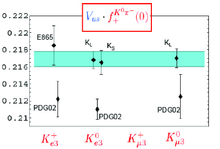
Figure 1: The quantity $V_{us}\times f_{+}(0)$ as extracted from various $K_{\ell 3}$ decay modes. The theoretical input needed to obtain these plots is discussed in the text. All the experimental input is taken from blucher-marciano . The shaded horizontal band represent the average over all modes (including correlations) with one-sigma error. For comparison, results based on ”old” (PDG02) $K_{\ell 3}$ measurements are also shown.

III.2 $B(D)\to P_{1}P_{2}$

Radiative corrections in heavy meson decays pose a harder theoretical problem, due to the lack of a universally valid effective theory (as it is ChPT in Kaon decays). Nonetheless, as remarked earlier, it is certainly possible to calculate the important IR effects using the approximation of point-like hadrons. A first step in this direction has been made in Ref. Baracchini:2005wp , that studied the non-leptonic decays $B(D)\to P_{1}P_{2}$ of heavy mesons into two pseudo-scalar mesons ($P_{1,2}=K,\pi$). In this work the electromagnetic interactions of hadrons are described by minimal coupling of the photon field to point-like pseudoscalar meson fields. The authors perform a complete $O(\alpha)$ calculation, which correctly captures the potentially large IR effects due to virtual and real photons. There is no attempt to perform a UV matching and to model the ”direct emission” of real photons. This implies an overall $O(\alpha/\pi)$ uncertainty in the final results and the impossibility to apply the results to emission of hard photons.

Despite these limitations, the analysis of Ref. Baracchini:2005wp has provided a definite improvement over existing calculations and MC implementations of radiative corrections for non-leptonic modes of heavy mesons. Moreover, it nicely illustrates the need to define an IR-safe observable, i.e. the necessity to give a prescription for the treatment of soft photons that always accompany charged decay products. The simplest definition of IR-safe observable Baracchini:2005wp involves a sum over the parent and radiative modes, with an upper cutoff on the energy carried by photons in the CMS of the decaying particle:

$$\Gamma^{\rm incl}_{H\to P_{1}P_{2}}(E^{\rm max})=\sum_{n}\Gamma(H\to P_{1}P_{2}+n\gamma)\Big{|}_{\sum E_{\gamma}<E^{\rm max}}~{}.$$ (10)

With the above definition, the explicit calculation leads to

$$\Gamma^{\rm incl}_{H\to P_{1}P_{2}}(E^{\rm max})=\Gamma^{0}_{H\to P_{1}P_{2}}\,G_{12}(E^{\rm max})$$ (11)

where $\Gamma^{0}_{H\to P_{1}P_{2}}$ represents the unobservable purely weak decay rate and $G_{12}(E^{\rm max})$ is the IR correction factor given to $O(\alpha)$ by:

$$G_{12}(E^{\rm max})=1+b\,\log\left(\frac{M_{H}}{2E^{\rm max}}\right)+c+O\left(\frac{E^{\rm max}}{M_{H}}\right)$$ (12)

where $b$ is the factor of Eq. 4 for the relevant decay mode and $c$ is a constant of $O(\alpha)$ fixed by the complete calculation of Ref. Baracchini:2005wp . In Fig. 2 I report the results for $G_{\pi\pi}$ and $G_{KK}$ in $B$ decays Baracchini:2005wp . The plot illustrates the importance to declare how the measured inclusive rate is defined: different definitions imply that one has to use different correction factors $G_{12}(E^{\rm max})$ to extract $\Gamma^{0}$ (and ultimately learn about the underlying weak and strong dynamics). For example, the correction factor is as large as $5\%$ in $B^{0}\to\pi^{+}\pi^{-}$ when $E^{\rm max}=250$ MeV.

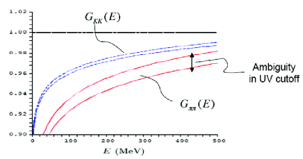
Figure 2: Examples of the e.m. correction factors for the photon-inclusive widths as a function of the cut on the maximal missing energy Baracchini:2005wp . The full lines represent $G_{\pi^{+}\pi^{-}}$ while the dashed lines represent $G_{K^{+}K^{-}}$ for the decays of $B$ mesons. In each case the upper curve is obtained by taking the renormalization scale $\mu=M_{\rho}$ while the lower curve for $\mu=M_{\pi}(M_{K})$. The difference is an estimate of the ambiguity entailed in the UV matching.

III.3 Factorization in $B\to\pi\ell\bar{\nu}_{\ell}\gamma$

Among radiative decays of heavy mesons, the mode $B\to\gamma\pi\ell\bar{\nu}_{\ell}$ offers one of the simplest testing-grounds of EFT tools. The hadronic dynamics of the radiative semileptonic decays is complicated by the presence of many energy scales. However, in certain kinematic regions a model independent treatment is possible. In the limit of a soft photon, Low’s theorem Low fixes the terms of order $O(q^{-1})$ and $O(q^{0})$ in the expansion of the decay amplitude in powers of the photon momentum $q$. Higher order terms in $q$ could be calculated with the help of the heavy hadron chiral perturbation theory wise ; BuDo ; TM ; review , as long as the pion and photon are sufficiently soft in the B rest-frame. This is the case in a limited corner of the phase space, corresponding to a large dilepton invariant mass $W^{2}=(p_{e}+p_{\nu})^{2}\sim m_{b}^{2}$. On the other hand, at low $W^{2}$ the decay $B\to\gamma\pi\ell\bar{\nu}_{\ell}$ produces in general either an energetic pion or an energetic photon (see Fig. 1). The non-trivial dynamics is encoded in the correlator of the weak semileptonic current with the electromagnetic current ($j_{\mu}^{\rm em}=\sum_{q}e_{q}\bar{q}\gamma_{\mu}q$)

$$T_{\mu\nu}(q)=i\int d^{4}xe^{iq.x}T\{(\bar{q}\gamma_{\nu}P_{L}b)(0)\,,j_{\mu}^{\rm e.m.}(x)\}.$$ (13)

Using soft-collinear effective theory (SCET) scet0 ; bfps ; scet2 ; scet3 -scet3.5 ; scet4 methods, it is possible to prove a factorization relation for the decay amplitude in the kinematic region with an energetic photon and a soft pion Cirigliano:2005ms . The hadronic matrix element of the correlator defined in Eq. 13 can then be written as

$$\langle\pi(p^{\prime})|T_{\mu\nu}(q)|\bar{B}(p)\rangle=C^{a}(E_{\gamma})\times$$

$$\int d\omega\,J(\omega)\,\times\langle\pi(p^{\prime})|O^{a}_{\mu\nu}(\omega)|\bar{B}(p)\rangle+O(\Lambda/Q)~{},$$ (14)

with $\Lambda\sim\Lambda_{QCD}$ and $Q\sim\{E_{\gamma},m_{b}\}$. Here $C^{a}$ and $J$ denote Wilson coefficients encoding the corrections coming respectively from hard and hard-collinear degrees of freedom and are therefore calculable in perturbation theory. $O^{a}_{\mu\nu}$ denote bi-local operators expressed in terms of $b$ and light-quark fields as well as soft Wilson lines. The above factorization relation holds for any process $B\to\gamma M\ell\nu$ ($M=\rho,\omega,\cdots$ a light soft meson) with the appropriate soft function $S(B\to M)$ replacing $\langle\pi(p^{\prime})|O^{a}_{\mu\nu}(\omega)|\bar{B}(p)\rangle$. The key point is that when $M=\pi$ we can use heavy hadron chiral perturbation theory wise ; BuDo ; TM ; review to relate the soft matrix elements $\langle\pi(p^{\prime})|O^{a}_{\mu\nu}(\omega)|\bar{B}(p)\rangle$ to $\langle 0|O^{a}_{\mu\nu}(\omega)|\bar{B}(p)\rangle$, that in turn can be expressed in terms of the B meson light-cone wave function $\phi_{+}^{B}(k_{+})$ GPchiral . The convolution of $\phi_{+}^{B}(k_{+})$ with the jet function $J$ in Eq. (14) is the main non-perturbative parameter characterizing $B\to\gamma\pi\ell\bar{\nu}_{\ell}$ to leading order in $\Lambda/Q$.

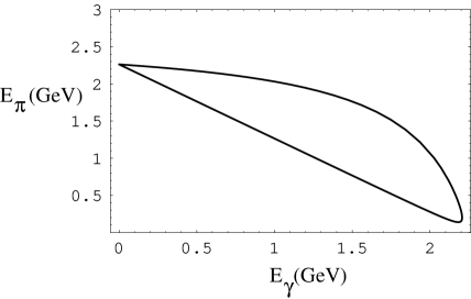
Figure 3: The Dalitz plot for $B\to\gamma\pi\ell\bar{\nu}$ at $W^{2}=4$ GeV². Our computation of the form factors is applicable in the lower right corner of the Dalitz plot, with an energetic photon and a soft pion.

In Ref. Cirigliano:2005ms we analyzed the above factorization formula, with a twofold intent: (i) give predictions for quantities such as photon spectrum and the integrated rate with appropriate cuts; (ii) compare our effective-theory based results with simplified approaches to $\bar{B}\to\pi e\bar{\nu}\gamma$, which are usually implemented in the Monte Carlo (MC) simulations used in the experimental analysis. In the numerical study we focused on the neutral B decay $\bar{B}^{0}\to\pi^{+}e^{-}\bar{\nu}_{e}\gamma$.

Factorization results
The theoretical tools used (SCET and HHChPT) force us to provide results for the photon energy spectrum, the distribution in the electron-photon angle, and integrated rate with various kinematic cuts:

1. An upper cut on the pion energy in the B rest frame $E_{\pi}<E_{\pi}^{\rm max}$, required by the applicability of chiral perturbation theory.

2. A lower cut on the charged lepton-photon angle in the rest frame of the $B$ meson, $\theta_{e\gamma}>\theta^{\rm min}_{e\gamma}$, required to regulate the collinear singularity introduced by photon radiation off the charged lepton.

3. Finally, to ensure the validity of the factorization theorem, we require the photon to be sufficiently energetic (in the $B$ rest frame) $E_{\gamma}^{\rm min}\gg\Lambda_{QCD}$. We choose $E_{\gamma}^{\rm min}=1$ GeV.

Working to leading order in $\alpha_{s}$ and in the chiral expansion, the non-perturbative quantities needed are: the first inverse moment of the light-cone B wave function $\phi_{+}^{B}(k_{+})$

$$\lambda_{B}^{-1}=\int dk_{+}\ \frac{\phi_{B}^{+}(k_{+},\mu)}{k_{+}}\ ,$$ (15)

the $B$ meson decay constant $f_{B}$, and the HHChPT $B-B^{*}-\pi$ coupling $g$. The numerical ranges used for the various input parameters parameters ; parameters1 ; parameters2 are summarized in Table 2.

The phase space integration with the cuts described above was performed using the Monte Carlo event generator RAMBO RAMBO . The factorization results for the photon energy spectrum and the distribution in $\cos\theta_{e\gamma}$ are shown in Fig. 4 (solid lines), using the central and extreme values for the input parameters as reported in Table 2. The shaded bands reflect the uncertainty in our prediction, which is due mostly to the variation of $\lambda_{B}$. For $E_{\gamma}^{\rm min}=1\ {\rm GeV}$, $E_{\pi}^{\rm max}=0.5\ {\rm GeV}$, and $\theta_{e\gamma}^{\rm min}=5^{o}$, the integrated radiative branching fraction predicted by our factorization formula is (up to small perturbative corrections in $\alpha_{s}(m_{b})$ and $\alpha_{s}(\sqrt{m_{b}\Lambda})$)

$${\rm Br}_{\bar{B}\to\pi e\bar{\nu}\gamma}^{\rm cut}({\rm fact}) = \Big{(}1.2\ \pm 0.2(g)\ ^{+2.2}_{-0.6}(\lambda_{B})\Big{)}\times 10^{-6}$$ (16)

$$\times \left(\frac{|V_{ub}|}{0.004}\right)^{2}\times\left(\frac{f_{B}}{200\ {\rm MeV}}\right)^{2}\ .$$

Apart from the overall quadratic dependence on $V_{ub}$ and $f_{B}$, the main uncertainty of this prediction comes from the poorly known non-perturbative parameter $\lambda_{B}$. It is worth mentioning that radiative rate, photon spectrum and angular distribution could be used in the future to obtain experimental constraints on $\lambda_{B}$, given their strong sensitivity to it. This requires, however, a reliable estimate of the impact of chiral corrections, $O(\alpha_{s})$ corrections, and the uncertainty in other input parameters.

Table 2: Input parameters used in the numerical computation parameters ; parameters1 ; parameters2 .

$f_{B}$	$(200\pm 30)$ MeV	$f_{\pi}$	$131$ MeV
$\lambda_{B}$	$(350\pm 150)$ MeV	$g$	$0.5\pm 0.1$
$|V_{ub}|$	$0.004$

Table 3: Branching fractions of the cut $\bar{B}\to\pi e\bar{\nu}\gamma$ decay corresponding to the factorization amplitude and the IB1, IB2 cases defined in the text, for central values of the input parameters reported in Table 2.

cuts	$10^{6}$ Br(fact)	$10^{6}$ Br(IB1)	$10^{6}$ Br(IB2)
$E_{\gamma}>1$ GeV
$E_{\pi}<0.5$ GeV	$1.2$	$2.4$	$2.8$
$\theta_{e\gamma}>5^{\circ}$

Figure 4: Left panel: Differential rate $d\bar{\Gamma}/dE_{\gamma}$, as a function of the photon energy in the $B$-meson rest frame. The normalization is given by $\bar{\Gamma}=10^{6}\,\Gamma_{B^{0}}^{-1}\times\Gamma(\bar{B}\to\pi e\bar{\nu}\gamma)$. Right panel: Differential radiative rate $d\bar{\Gamma}/d(\cos\theta_{e\gamma})$, as a function of the cosine of electron-photon angle in the $B$-meson rest frame. The shaded bands and the superimposed continuous lines represent the uncertainty in the factorization result (FACT) induced by the parameter $\lambda_{B}$, assumed to range between 200 (upper line) and 500 (lower line) MeV, with all other parameters equal to the central values of Table 2. The dark(light)-gray dashed line corresponds to the IB1 (IB2) results (see text for their definition).

Comparison with simplified approaches
In the Monte Carlo simulations used in most experimental analyses of B decays, simplified versions of the radiative hadronic matrix elements are implemented. These rely essentially on Low’s theorem Low and are valid only in the limit of soft photons ($E_{\gamma}\ll\Lambda$). They are nonetheless used over the entire kinematic range, for lack of better results. Our interest here is to evaluate how these methods fare in the region of soft pion and hard photon (certainly beyond their regime of validity), where we can use the QCD-based factorization results as benchmark.

We use two simplified versions of the $\bar{B}\to\pi e\bar{\nu}\gamma$ matrix element, which we denote IB1 and IB2.

• This is the $O(q^{-1})$ component of Low’s amplitude. The PHOTOS Monte Carlo photos implements this form of the radiative amplitude.

• This corresponds to a tree-level calculation with point-like $B$ and $\pi$, and a constant transition form factor Ginsberg .

The results for the photon energy spectrum and the distribution in $\cos\theta_{e\gamma}$ are shown in Figs. 4 (IB1: dark-gray dashed lines, IB2: light-gray dashed lines). The integrated branching fractions are listed in Table 3 (together with the factorization prediction) for central values of the input parameters given in Table 2. The IB1 and IB2 branching fractions scale very simply with the input parameters, being proportional to $(|V_{ub}|\,g\,f_{B})^{2}$. As can be seen from the comparison of differential distributions and BRs, the two cases IB1 and IB2 lead to almost identical predictions, which are, however, quite different from the factorization ones. For central values of the input parameters reported in Table 2 the IB1 and IB2 predict a radiative BR roughly a factor of two larger than the factorization result. Moreover, the shape of the distributions in $E_{\gamma}$ and $\cos\theta_{e\gamma}$ are quite different. We hope that our results can help construct more reliable MCs for the simulation of $\bar{B}\to\pi e\bar{\nu}\gamma$ decays, or at least address the systematic uncertainty to be assigned to the present MC results.

IV Conclusions

In this talk I have reviewed recent developments in the calculation of radiative corrections to $K$ and $B$ decays, arguing that control of radiative effects is mandatory in order to make meaningful phenomenology at the few $\%$ level.

The situation in $K$ decays is satisfactory, because the chiral expansion provides a robust tool to calculate radiative corrections and estimate the residual uncertainties.

In $B$ and $D$ decays there is no ”universal” effective theory that can be invoked. Rigorous treatments are possible only in limited regions of phase space. For those modes in which experimental precision will reach the few $\%$ level in the near future, the minimal goal is to perform complete $O(\alpha)$ calculation in the approximation of point-like hadrons. This should at least capture the leading IR effects, that are known to be large in some modes Baracchini:2005wp . Whenever possible, it is desirable to perform calculations within the appropriate hadronic effective theory. This will help assessing the uncertainty entailed in the point-like approximation and in the Monte Carlo simulations presently used in experimental analyses. As an example of EFT calculation, I have discussed the process $\bar{B}\to\pi e\bar{\nu}\gamma$ in the regime of soft pion and hard photon Cirigliano:2005ms .