Hadronic $B$ decays from SCET

Abstract

In this talk I will discuss non-leptonic $B$ decays, in particular how soft-collinear effective field theory (SCET) can be used to constrain the non-perturbative hadronic parameters required to describe the various observables.

I Introduction

The standard model (SM) of particle physics has proven to hold up against any experimental tests it has been subjected to so far. The SM has several striking features for which no underlying principle has been experimentally confirmed to this date. First, the SM requires the scale of electro-weak symmetry breaking to be of order a few hundred GeV, which is many orders of magnitude below the only fundamental scale of nature we know of, the Planck scale. Second, to explain the masses and flavor violating transitions of fermions requires the fundamental Yukawa matrices to satisfy a very particular scaling, for which no satisfactory symmetry or other underlying principle has been found so far. While the scale of electro-weak symmetry breaking is known from the measured properties of gauge interactions, the scale of flavor violation could be completely unrelated to that scale. However, many models of new physics which address the electro-weak scale also give additional contributions to flavor physics. Thus, precise measurements of flavor and CP violating observables can severely constrain possible models of electro-weak symmetry breaking.

Since the standard model predicts the short distance couplings of quarks to one another, while experimental measurements are done with hadrons, one needs to understand long distance QCD effects on the measured quantities to extract the underlying physics. It is the purpose of this talk to discuss how this separation between long and short distance physics can be achieved using effective theories. The effective theory that is applicable to the non-leptonic $B$ decays to two light mesons, as we are concerned with here, is the soft-collinear effective theory (SCET) SCET .

II Factorization in $B\to M_{1}M_{2}$

There has been tremendous progress over the last few years in understanding charmless two-body, non-leptonic $B$ decays in the heavy quark limit of QCD QCDF ; PQCD ; pipiChay ; bprs ; Bauer:2001cu ; pQCDKpi ; BW . In this limit one can prove factorization theorems of the matrix elements describing the strong dynamics of the decay into simpler structures such as light cone distribution amplitudes of the mesons and matrix elements describing a heavy to light transition QCDF . It is very important that these results are obtained from a systematic expansion in powers of $\Lambda_{\rm QCD}/m_{b}$. The development of soft-collinear effective theory (SCET) SCET allowed these decays to be treated in the framework of effective theories, clarifying the separation of scales in the problem, and allowing factorization to be generalized to all orders in $\alpha_{s}$.

Factorization for $B\to M_{1}M_{2}$ decays involves three distinct distance scales $m_{b}^{2}\gg E_{M}\Lambda\gg\Lambda^{2}$. For $B\to M_{1}M_{2}$ decays, a factorization theorem was proposed by Beneke, Buchalla, Neubert and Sachrajda QCDF , often referred to as the QCDF result in the literature. Another proposal is a factorization formula which depends on transverse momenta, which is referred to as PQCD PQCD . The factorization theorem derived using SCET bprs ; pipiChay agrees with the structure of the QCDF proposal if perturbation theory is applied at the scales $m_{b}^{2}$ and $m_{b}\Lambda$. One of the differences is that QCDF treats $c\bar{c}$ penguins perturbatively, while in the SCET analysis they are left as a perturbative contribution plus an unfactorized large ${\cal O}(v)$ term. The SCET result improved the factorization formula by generalizing it to allow each of the scales $m_{b}^{2}$, $E_{M}\Lambda$, and $\Lambda^{2}_{\rm QCD}$ to be discussed independently.

The derivation of the SCET factorization theorem occurs in several steps, corresponding to integrating out the various scales in the problem. As already mentioned, the relevant scales are $\mu\sim m_{b}$, $\mu\sim\sqrt{m_{b}\Lambda_{\rm QCD}}$ and $\mu\sim\Lambda_{\rm QCD}$. One starts from the effective weak Hamiltonian, which describes the effects of the weak physics in terms of local 4-quark operators. Integrating out $\sim m_{b}$ fluctuations, the effective Hamiltonian at leading order in ${\rm SCET}_{\rm I}$ bps4 can be written schematically as

$$H_{W}\!\! = \!\!\frac{2G_{F}}{\sqrt{2}}\sum_{i}\left[c_{i}\otimes Q_{i}^{(0)}+b_{i}\otimes Q_{i}^{(1)}+{\cal Q}_{c\bar{c}}\right]\,,$$ (1)

where $c_{i}$ and $b_{i}$ are Wilson coefficients, and the symbol $\otimes$ denotes convolutions over various momentum fractions.

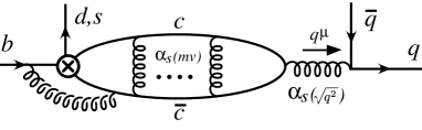
Figure 1: Example of long distance charming penguins. The $mv$ gluons are nonperturbative and LO soft gluons are exchanged by the $b$, $c$, $\bar{c}$ and spectator quark which is not shown.

The term ${\cal Q}_{c\bar{c}}$ denotes operators appearing in long distance charm effects as in Fig. 1. There is broad agreement that charm loop contributions from hard ($\sim\!m_{b}$) momenta can be computed in perturbation theory and they are included in the $c_{i}$ and $b_{i}$ coefficients in Eq. (1). However, there are non-perturbative contributions from penguin charm quark loops (so-called charming penguins cpens ), which are contained in ${\cal Q}_{c\bar{c}}$. While no proof of factorization for the matrix element of this operator exists, it is still possible to determine its parametric dependence on $m_{c}/m_{b}$, $v$, and $\Lambda_{\rm QCD}/m_{b}$ using operators in effective field theories. We find

$$\frac{A_{c\bar{c}}^{\pi\pi}}{A^{\pi\pi}_{LO}}\sim\alpha_{s}(2m_{c})\>f\Big{(}\frac{2m_{c}}{m_{b}}\Big{)}\>v\,,$$ (2)

Thus, this contribution gives rise to a source of strong phases in the amplitudes, while all strong phases vanish for the other terms. For this reason, we will keep this term and treat its matrix element as an unknown complex parameter in the theory.

The collinear fields in the operators $O_{i}^{(0,1)}$ can be decoupled from the ultrasoft fields by making a simple field redefinition SCET . The operators $O_{i}^{(0,1)}$ then factor into $(n,v)$ and ${\bar{n}}$ parts,

$$Q_{i}^{(0,1)}=\tilde{Q}_{i}^{(0,1)}Q_{i}^{\bar{n}}\,.$$ (3)

The first term contains both a soft $b$ quark field and a collinear field in the ${\bar{n}}$ direction, while the second term contains two collinear fields in the $n$ direction. The matrix element of the operators $O_{i}^{(0,1)}$ thus factor into a $B\to M$ transition matrix element, and a vacuum to light meson matrix element.

Putting all these results together, we obtain the SCET factorization formula

$$A\!\! = \!\!\frac{G_{F}m_{B}^{2}}{\sqrt{2}}\!\bigg{[}\bigg{\{}f_{M_{1}}\!\int_{0}^{1}\!\!\!\!du\,dz\,T_{1\!J}(u,z)\zeta^{BM_{2}}_{J}(z)\phi^{M_{1}}(u)$$ (4)

$$+f_{M_{1}}\zeta^{BM_{2}}\!\!\int_{0}^{1}\!\!\!\!du\,T_{1\zeta}(u)\phi^{M_{1}}(u)\bigg{\}}\!+\!\Big{\{}1\leftrightarrow 2\Big{\}}$$

$$+\lambda_{c}^{(f)}A_{c\bar{c}}^{M_{1}M_{2}}\bigg{]},$$

where $\zeta^{BM}$ and $\zeta^{BM}_{J}$ are non-perturbative parameters describing $B\to M$ transition matrix elements, and $A_{\rm c\bar{c}}^{M_{1}M_{2}}$ parameterizes complex amplitudes from charm quark contractions for which factorization has not been proven. Power counting implies $\zeta^{BM}\sim\zeta^{BM}_{J}\sim(\Lambda/Q)^{3/2}$. $T_{1\!J}(u,z)$ and $T_{1\zeta}(u)$ are perturbatively calculable in an expansion in $\alpha_{s}(m_{b})$ and depend upon the process of interest.

At leading order in $\alpha_{s}(m_{b})$ the short distance coefficients $T_{1\!J}(u,z)$ is independent of the parameter $z$, which implies that the functional form of the non-perturbative function $\zeta_{J}^{BM}(z)$ does not matter, since we can define a new hadronic parameter $\zeta_{J}^{BM}\equiv\int\!dz\,\zeta_{J}^{BM}(z)$.

III Phenomenology

III.1 Counting of hadronic parameters

Without any theoretical input, there are 4 real hadronic parameters for each decay mode (one complex amplitude for each CKM structure) minus one overall strong phase. In addition, there are the weak CP violating phases that we want to determine. For $B\to\pi\pi$ decays there are a total of 11 hadronic parameters, while in $B\to K\pi$ decays there are 15 hadronic parameters.

Using isospin, the number of parameters is reduced. Isospin gives one amplitude relation for both the $\pi\pi$ and the $K\pi$ system, thus eliminating 4 hadronic parameters in each system (two complex amplitudes for each CKM structure). This leaves 7 hadronic parameters for $B\to\pi\pi$ and 11 for $B\to K\pi$.

The SU(3) flavor symmetry relates not only the decays $B\to\pi\pi$ and $B\to K\pi$, $B\to KK$, but also $B\to\pi\eta_{8}$, $B\to\eta_{8}K$ and $B_{s}$ decays to two light mesons. The decomposition of the amplitudes in terms of SU(3) reduced matrix elements can be obtained from Zeppenfeld ; SavageWise ; GrinsteinLebed . and 20 hadronic parameters are required to describe all these decays minus 1 overall phase (plus additional parameters for singlets and mixing to properly describe $\eta$ and $\eta^{\prime}$). Of these hadronic parameters, only 15 are required to describe $B\to\pi\pi$ and $B\to K\pi$ decays (16 minus an overall phase). If we add $B\to KK$ decays then 4 more paramaters are needed (which are solely due to electroweak penguins).

	no			SCET	SCET
	expn.	SU(2)	SU(3)	+SU(2)	+SU(3)
$B\to\pi\pi$	11	7/5		4
$B\to K\pi$	15	11	15/13	+5(6)	4
$B\to K\bar{K}$	11	11	+4/0	+3(4)	+0

Table 1: Number of real hadronic parameters from different expansions in QCD. The first column shows the number of theory inputs with no approximations, while the next columns show the number of parameters using only SU(2), using only SU(3), using SU(2) and SCET, and using SU(3) with SCET. For the cases with two numbers, $\#/\#$, the second follows from the first after neglecting the small penguin coefficients, ie setting $C_{7,8}=0$. In SU(2) + SCET $B\to K\pi$ has 6 parameters, but 1 appears already in $B\to\pi\pi$, hence the $+5(6)$. The notation is analogous for the $+3(4)$ for $B\to K\bar{K}$.

The number of parameters that occur at leading order in different expansions of QCD are summarized in Table 1, including the SCET expansion. The parameters with isospin+SCET are

$$\pi\pi: \{\zeta^{B\pi}\!+\!\zeta_{J}^{B\pi},\beta_{\pi}\zeta_{J}^{B\pi},P_{\pi\pi}\}\,,$$ (5)

$$K\pi: \{\zeta^{B\pi}\!+\!\zeta_{J}^{B\pi},\beta_{\bar{K}}\zeta_{J}^{B\pi},\zeta^{B\bar{K}}+\zeta_{J}^{B\bar{K}},\beta_{\pi}\zeta_{J}^{B\bar{K}},P_{K\pi}\}\,,$$

$$K\bar{K}: \{\zeta^{B\bar{K}}+\zeta_{J}^{B\bar{K}},\beta_{K}\zeta_{J}^{B\bar{K}},P_{K\bar{K}}\}\,.$$

Here $P_{M_{1}M_{2}}$ are complex penguin amplitudes and the remaining parameters are real.

Taking SCET + SU(3) we have the additional relations $\zeta^{B\pi}=\zeta^{BK}=\zeta^{B\bar{K}}$, $\zeta_{J}^{B\pi}=\zeta_{J}^{BK}=\zeta_{J}^{B\bar{K}}$, $\beta_{\pi}=\beta_{K}=\beta_{\bar{K}}$, and $A_{cc}^{\pi\pi}=A_{cc}^{K\pi}=A_{cc}^{K\bar{K}}$ which reduces the number of parameters considerably.

III.2 Implications of small phases

In SCET, the only source of strong phases are from the charm penguin amplitude parameter $A_{cc}$. Since by SU(2) flavor symmetry there is only a single such amplitude parameter for the decays $B\to K\pi$, all relative strong phases between $A_{cc}$ and any other term are the same, while relative strong phases between any other two amplitude parameters are identically zero. This result can be used to make several predictions in SCET, which are relatively independent of the actual size of the value of the amplitude parameters. An example are certain sum rules in the decays $B\to K\pi$, which are constructed out of the ratios of brancing ratios

$$R_{1} = \frac{2{\rm Br}(B^{-}\to\pi^{0}K^{-})}{{\rm Br}(B^{-}\to\pi^{-}\bar{K}^{0})}-1\,,$$ (6)

$$R_{2} = \frac{{\rm Br}(\bar{B}^{0}\to\pi^{-}K^{+})\tau_{B^{-}}}{{\rm Br}(B^{-}\to\pi^{-}\bar{K}^{0})\tau_{B^{0}}}-1\,,$$

$$R_{3} = \frac{2{\rm Br}(\bar{B}^{0}\to\pi^{0}\bar{K}^{0})\tau_{B^{-}}}{{\rm Br}(B^{-}\to\pi^{-}\bar{K}^{0})\tau_{B^{0}}}-1\,,$$

and rescaled asymmetries

$$\Delta_{1} = (1+R_{1})A_{\rm CP}(\pi^{0}K^{-})\,,$$ (7)

$$\Delta_{2} = (1+R_{2})A_{\rm CP}(\pi^{-}K^{+})\,,$$

$$\Delta_{3} = (1+R_{3})A_{\rm CP}(\pi^{0}\bar{K}^{0})\,,$$

$$\Delta_{4} = A_{\rm CP}(\pi^{-}\bar{K}^{0})\,.$$

They can be combined into linear combinations, which satisfy

$$R_{1}-R_{2}+R_{3}\sim{\cal O}(\epsilon^{2})$$ (8)

and

$$\Delta_{1}-\Delta_{2}+\Delta_{3}-\Delta_{4}\sim\epsilon^{2}\sin\gamma\sin(\Delta\phi)$$ (9)

Here $\epsilon$ denotes a small parameter that is either proportional to $\lambda_{u}/\lambda_{c}$ or $C_{9,10}/C_{4}$. Thus, these combinations of parameters are expected to give contributions which are much smaller than each of the individual terms. Furthermore, the fact that the sum rule for the CP asymmetries is proportional to the differences of strong phases, reduces the predicted result in SCET even more.

Table 2: Predicted CP averaged branching ratios ($\times 10^{-6}$, first row) and direct CP asymmetries (second row for each mode) for $\Delta S=0$ and $\Delta S=1$ $B$ decays (separated by horizontal line) to isosinglet pseudoscalar mesons. The Theory I and Theory II columns give predictions corresponding to two possible solutions for the hadronic parameters. The errors on the predictions are estimates of SU(3) breaking, $1/m_{b}$ corrections and errors due to SCET parameters, respectively. No prediction on CP asymmetries is given, if $[-1,1]$ range is allowed at $1\sigma$.

Mode	Exp.	Theory I	Theory II
$B^{-}\to\pi^{-}\eta$	$4.3\pm 0.5\;(S=1.3)$	$4.9\pm 1.7\pm 1.0\pm 0.5$	$5.0\pm 1.7\pm 1.2\pm 0.4$
	$-0.11\pm 0.08$	$0.05\pm 0.19\pm 0.21\pm 0.05$	$0.37\pm 0.19\pm 0.21\pm 0.05$
$B^{-}\to\pi^{-}\eta^{\prime}$	$2.53\pm 0.79\;(S=1.5)$	$2.4\pm 1.2\pm 0.2\pm 0.4$	$2.8\pm 1.2\pm 0.3\pm 0.3$
	$0.14\pm 0.15$	$0.21\pm 0.12\pm 0.10\pm 0.14$	$0.02\pm 0.10\pm 0.04\pm 0.15$
$\bar{B}^{0}\to\pi^{0}\eta$	$<2.5$	$0.88\pm 0.54\pm 0.06\pm 0.42$	$0.68\pm 0.46\pm 0.03\pm 0.41$
	$-$	$0.03\pm 0.10\pm 0.12\pm 0.05$	$-0.07\pm 0.16\pm 0.04\pm 0.90$
$\bar{B}^{0}\to\pi^{0}\eta^{\prime}$	$<3.7$	$2.3\pm 0.8\pm 0.3\pm 2.7$	$1.3\pm 0.5\pm 0.1\pm 0.3$
	$-$	$-0.24\pm 0.10\pm 0.19\pm 0.24$	$-$
$\bar{B}^{0}\to\eta\eta$	$<2.0$	$0.69\pm 0.38\pm 0.13\pm 0.58$	$1.0\pm 0.4\pm 0.3\pm 1.4$
	$-$	$-0.09\pm 0.24\pm 0.21\pm 0.04$	$0.48\pm 0.22\pm 0.20\pm 0.13$
$\bar{B}^{0}\to\eta\eta^{\prime}$	$<4.6$	$1.0\pm 0.5\pm 0.1\pm 1.5$	$2.2\pm 0.7\pm 0.6\pm 5.4$
	$-$	$-$	$0.70\pm 0.13\pm 0.20\pm 0.04$
$\bar{B}^{0}\to\eta^{\prime}\eta^{\prime}$	$<10$	$0.57\pm 0.23\pm 0.03\pm 0.69$	$1.2\pm 0.4\pm 0.3\pm 3.7$
	$-$	$-$	$0.60\pm 0.11\pm 0.22\pm 0.29$
$\bar{B}^{0}\to\bar{K}^{0}\eta^{\prime}$	$63.2\pm 4.9\;(S=1.5)$	$63.2\pm 24.7\pm 4.2\pm 8.1$	$62.2\pm 23.7\pm 5.5\pm 7.2$
	$0.07\pm 0.10\;(S=1.5)$	$0.011\pm 0.006\pm 0.012\pm 0.002$	$-0.027\pm 0.007\pm 0.008\pm 0.005$
$\bar{B}^{0}\to\bar{K}^{0}\eta$	$<1.9$	$2.4\pm 4.4\pm 0.2\pm 0.3$	$2.3\pm 4.4\pm 0.2\pm 0.5$
	$-$	$0.21\pm 0.20\pm 0.04\pm 0.03$	$-0.18\pm 0.22\pm 0.06\pm 0.04$
$B^{-}\to K^{-}\eta^{\prime}$	$69.4\pm 2.7$	$69.5\pm 27.0\pm 4.3\pm 7.7$	$69.3\pm 26.0\pm 7.1\pm 6.3$
	$0.031\pm 0.021$	$-0.010\pm 0.006\pm 0.007\pm 0.005$	$0.007\pm 0.005\pm 0.002\pm 0.009$
$B^{-}\to K^{-}\eta$	$2.5\pm 0.3$	$2.7\pm 4.8\pm 0.4\pm 0.3$	$2.3\pm 4.5\pm 0.4\pm 0.3$
	$-0.33\pm 0.17\;(S=1.4)$	$0.33\pm 0.30\pm 0.07\pm 0.03$	$-0.33\pm 0.39\pm 0.10\pm 0.04$

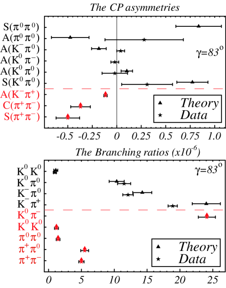
Figure 2: Comparison of theory and experiment for all available data in $B\to\pi\pi$ and $B\to K\pi$ decays, with $\gamma=83^{\circ}$. The 8 pieces of data in red (below the dashed line) have been used to determine the SCET hadronic parameters $\zeta^{B\pi}$, $\zeta_{J}^{B\pi}$, $P_{\pi\pi}$ as described in the text. The data above the line are predictions. The CP asymmetry in $B^{-}\to K^{0}\pi^{-}$ is expected to be small, but its numerical value is not predicted reliably.

Experimentally, one finds

$$R_{1}-R_{2}+R_{3}=(0.19\pm 0.15)^{\rm expt}$$

$$\Delta_{1}-\Delta_{2}+\Delta_{3}-\Delta_{4}=(0.14\pm 0.15)^{\rm expt}\,,$$ (10)

and these results are consistent with zero. The SCET predictions are considerably more precise than the current measurements, and using conservative ranges $\zeta^{B\pi}+\zeta^{B\pi}_{J}=0.2\pm 0.1$, $\beta_{\bar{K}}\zeta_{J}^{B\pi}=0.10\pm 0.05$, $\zeta^{B\bar{K}}+\zeta^{B\bar{K}}_{J}=0.2\pm 0.1$, $\beta_{\pi}\zeta_{J}^{B\bar{K}}=0.10\pm 0.05$, $\gamma=70^{\circ}\pm 15^{\circ}$,and all phase differences $\Delta\phi=0^{\circ}\pm 30^{\circ}$ one finds

$$R_{1}-R_{2}+R_{3}=0.028\pm 0.021\,,$$ (11)

and for the CP-sum rule

$$\Delta_{1}-\Delta_{2}+\Delta_{3}-\Delta_{4}=0\pm 0.013\,.$$ (12)

Experimental deviations that are larger than these would be a signal for new physics.

III.3 General analysis for $B\to\pi\pi$, $B\to K\pi$ decays

From Table 1 and Eq. (5) we can see that a total of 12 hadronic parameters are required to describe the decays $B\to\pi\pi$, $B\to K\pi$ and $B\to KK$ at leading order in SCET. On top of that, there is one weak phase $\gamma$ which we will take as an unknown parameter. However, in both the decays $B\to K\pi$ and $B\to KK$, the coefficients multiplying the $B\to K$ transition matrix elements $\zeta^{BK}$ and $\zeta_{J}^{BK}$ are very small, which implies that the observables are insensitive to the numerical value of these hadronic matrix elements. This eliminates three of the hadronic parameters, namely $\zeta^{BK}+\zeta_{J}^{BK}$, $\beta_{\pi}\zeta_{J}^{BK}$ and $\beta_{K}\zeta_{J}^{BK}$. Finally, if we take the inverse moments of pion and kaon wave functions as experimental input, we obtain one additional relation between hadronic parameters. This leaves us with a total of 7 hadronic parameters as well as one weak phase. The 8 measurements used to fix these parameters are the branching ratios for $B$ decays to $\pi^{+}\pi^{-}$, $\pi^{+}\pi^{0}$, $\pi^{0}\pi^{0}$, $K^{0}K^{0}$, $K^{0}\pi^{-}$, as well as the CP asymmetries $S(\pi^{+}\pi^{-})$, $C(\pi^{+}\pi^{-})$ and $A_{\rm CP}(K^{-}\pi^{+})$.

Using the hadronic parameters extracted from the $B\to\pi\pi$ decays ($\zeta^{B\pi}$, $\zeta_{J}^{B\pi}$ and $P_{\pi\pi}$), the value for $P_{K\pi}$ determined from the decays $B^{-}\to\pi^{-}\bar{K}^{0}$ and $\bar{B}^{0}\to\pi^{-}K^{+}$ decays and independently varying $\zeta^{BK}+\zeta^{BK}_{J}=0.2\pm 0.1$ and $\beta_{\pi}\zeta^{BK}_{J}=0.10\pm 0.05$, we can calculate all the remaining currently measured $K\pi$ observables. The results are shown in Fig. 2. The data used in the fit are shown in red below the dashed dividing line while those above the line are predictions. Note that there is one more piece of data below the line than there are hadronic parameters. This additional experimental information was used to determine the value $\gamma=83^{\circ}$.

We see that $\gamma=83^{\circ}$ gives a good match to the $B\to\pi\pi$ data except for the asymmetry $C(\pi^{0}\pi^{0})$. When taking into account the theoretical error the most striking disagreements are the ${\rm Br}(K^{-}\pi^{+})$ at $2.3\sigma$ and the CP-asymmetry $A_{\rm CP}(K^{-}\pi^{0})$ at $2.6\sigma$. All other predictions agree within the uncertainties. Note that one could demand that $A_{\rm CP}(K^{-}\pi^{0})$ be reproduced, which would imply a negative value of $\zeta_{J}^{BK}$ (a naive fit for $\gamma=83^{\circ}$ gives $\zeta_{J}^{BK}\sim-0.15$). Note however, that this would imply that both perturbation theory at the intermediate scale $\mu=\sqrt{E\Lambda}$ and SU(3) are badly broken.

III.4 Including isosinglet mesons

The above analysis has recently been repeated to include decays to iso-singlet final states ZW . This requires adding additional contributions which arise from purely gluonic configurations. It turns out that the additional operators do not change the form of the factorization theorem given in Eq. (4), but the hadronic parameters $\zeta$, $\zeta_{J}$ and $A_{cc}$ receive order one contributions from these additional operators. To add isosinglet mesons to the phenomenological analysis thus requires a second set of parameters $\zeta_{g}$, $\zeta_{J,g}$ and $A_{cc,g}$, which have to be determined from data separately. Since experimentally there are not enough decays available, SU(3) flavor symmetry is required to retain predictive power. At the present time, there are two solutions possible for the gluonic hadronic parameters, and the degeneracy can only be lifted with further data. The results of the global fit, as taken from ZW , are shown in Table 2.

IV Conclusions

In this talk I have discussed how one can separate the long distance non-perturbative physics from the underlying short distance physics using the soft-colinear effective theory. One finds that the number of hadronic parameters is significantly reduced, such that they can be extracted directly from a subset of the data, and then used to make predictions for the remaining data. I have given a brief discussion of the factorization theorem as it emerges from SCET, and then discussed three phenomenological applications. First, I gave a detailed counting of the hadronic parameters using various theoretical approaches, then I discussed a few impacts of the fact that there is only one source of strong phases in the decay amplitudes, and finally, I showed results for global analyses of $B$ decays to two pseudoscalar mesons, with and without including isosinglet mesons.

References

• (1) C. W. Bauer, S. Fleming and M. E. Luke, Phys. Rev. D 63, 014006 (2001); C. W. Bauer, S. Fleming, D. Pirjol and I. W. Stewart, Phys. Rev. D 63, 114020 (2001); C. W. Bauer and I. W. Stewart, Phys. Lett. B 516, 134 (2001); Phys. Rev. D 65, 054022 (2002); C. W. Bauer, S. Fleming, D. Pirjol, I. Z. Rothstein and I. W. Stewart, Phys. Rev. D 66, 014017 (2002).
• (2) M. Beneke, G. Buchalla, M. Neubert and C. T. Sachrajda, Phys. Rev. Lett.  83, 1914 (1999) [arXiv:hep-ph/9905312]; Nucl. Phys. B 591, 313 (2000) [arXiv:hep-ph/0006124]; M. Beneke, G. Buchalla, M. Neubert and C. T. Sachrajda, Nucl. Phys. B 606, 245 (2001) [arXiv:hep-ph/0104110]; M. Beneke and M. Neubert, Nucl. Phys. B 675, 333 (2003) [arXiv:hep-ph/0308039].
• (3) Y.Y. Keum et al, Phys. Lett. B 504, 6 (2001); Phys. Rev. D 63, 054008 (2001); C. D. Lu et al., Phys. Rev. D 63, 074009 (2001).
• (4) C. W. Bauer, D. Pirjol, I. Z. Rothstein and I. W. Stewart, Phys. Rev. D 70, 054015 (2004) [arXiv:hep-ph/0401188].
• (5) J. g. Chay and C. Kim, Phys. Rev. D 68, 071502 (2003) [arXiv:hep-ph/0301055]; Nucl. Phys. B 680, 302 (2004) [arXiv:hep-ph/0301262].
• (6) C. W. Bauer, D. Pirjol and I. W. Stewart, Phys. Rev. Lett.  87, 201806 (2001) [arXiv:hep-ph/0107002].
• (7) H. n. Li, S. Mishima and A. I. Sanda, arXiv:hep-ph/0508041.
• (8) C. N. Burrell and A. R. Williamson, arXiv:hep-ph/0504024.
• (9) C.W. Bauer, D. Pirjol and I.W. Stewart, Phys. Rev. D 67, 071502 (2003).
• (10) M. Ciuchini, E. Franco, G. Martinelli and L. Silvestrini,Nucl. Phys. B 501, 271 (1997); M. Ciuchini et al., Phys. Lett. B 515, 33 (2001). M. Ciuchini et al., arXiv:hep-ph/0208048. P. Colangelo, G. Nardulli, N. Paver and Riazuddin, Z. Phys. C 45, 575 (1990).
• (11) D. Zeppenfeld, Z. Phys. C 8, 77 (1981).
• (12) M. J. Savage and M. B. Wise, Phys. Rev. D 39, 3346 (1989) [Erratum-ibid. D 40, 3127 (1989)].
• (13) B. Grinstein and R. F. Lebed, Phys. Rev. D 53, 6344 (1996) [arXiv:hep-ph/9602218].
• (14) A. R. Williamson and J. Zupan, arXiv:hep-ph/0601214.