Measuring C-odd correlations at lepton-proton and photon-proton collisions

Abstract

We consider the charge-odd correlations (COC) in cross sections of processes of production of charged particles. The cases of a muonic pair and pion systems $\pi^{+}\pi^{-}$, $\pi^{+}\pi^{-}\pi^{0}$ are considered in detail for electron-proton or photon-proton collisions in the proton fragmentation region kinematics. COC arise from interference of amplitudes which describe the different mechanisms of charged leptons (pions) creation. One of them corresponds to production of particles in the charge-odd state (one virtual photon or vector meson annihilation to this system of particles) and the other corresponds to the charge-even state of produced particles (creation by two photons). COC for muon-antimuon pair creation have a pure QED nature and can be considered as a normalization process. The processes with pion production are sensitive to some characteristics of proton wave functions and, besides, can be used for checking the anomalous and normal parts of the effective pionic lagrangian.

Three electromagnetic currents operator matrix element can be measured in photon-proton interactions with lepton pair production. For this aim a charge-odd combination of cross sections can be constructed as a conversion of leptonic 3-rank tensor with hadronic ones. These experiments can be considered as an alternative to deep virtual Compton scattering.

I Introduction

We want attract an attention to problem of experimental studies of anomalies of meson lagrangian. Wess-Zumino-Witten effective meson lagrangian BKK (it’s anomalous part) contains four types of anomalies: $\pi^{0}\to 2\gamma$, $\gamma^{*}\to 3\pi$, $\gamma\gamma\to 3\pi$, $K\bar{K}\to 3\pi$. First two of them was experimentally studied up to now (a lot of information about $\pi^{0}\to 2\gamma$ and rather poor one about $\gamma^{*}\to 3\pi$). But last two of them wasn’t investigated before. In experiments with fragmentation region kinematics the anomalous vertex $\gamma\gamma\to 3\pi$ can be measured. That is one of the main purpose of our paper.

In papers hpst1 ; hpst2 ; hpst3 the asymmetries of two pion production was investigated with the use of QCD lagrangian based approach. The main attention there was paid to differential distributions on azimuthal angles and invariant mass of pion pair produced in pionization region. This kinematics permits one to investigate C-odd interference of two and three gluon exchange mechanisms.

In our paper we use alternative approach based on Wess-Zumino-Witten effective meson lagrangian expressed in terms of hadronic fields. We obtained distributions on energy fractions of pions in fragmentation region if initial proton.

The charge-odd contribution to cross section of processes

$$e^{-}(p_{1})+p(p) \to e^{-}(p_{1}^{\prime})+p(p^{\prime})+\mu^{-}(q_{-})+\mu^{+}(q_{+}),$$

$$e^{-}(p_{1})+p(p) \to e^{-}(p_{1}^{\prime})+p(p^{\prime})+\pi^{-}(q_{-})+\pi^{+}(q_{+}),$$ (1)

$$e^{-}(p_{1})+p(p) \to e^{-}(p_{1}^{\prime})+p(p^{\prime})+\pi^{-}(q_{-})+\pi^{+}(q_{+})+\pi^{0}(q_{0}),$$

is caused by interference of amplitudes describing the two-photon mechanism and one photon mechanism of meson set production (see Fig. 1, a, b).

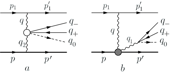
Figure 1: The mechanisms of production of muons (pions) pair and three pions state.

The similar quantity can be constructed for inelastic collisions of photon with hadron with production of lepton pairs. The properties of effective meson lagrangian as well as three-current correlators matrix elements, averaged on hadron states can be measured in relevant experiments, which is a motivation of our paper. We consider below the experimental set-up corresponding to the kinematical region of proton fragmentation,which means that the recoil proton and mesons created move in directions close to the initial proton motion in the center of mass system of initial particles, with invariant mass square of this jet $s_{1}$ much smaller than the center of mass square of the total energy of initial particles $s+M^{2}$ ($M$ is proton mass,we put below the electron mass as well as $\mu$ and $\pi$ meson masses $m$ to be small and neglect the terms of order $m^{2}/s_{1}$, $s_{1}/s$).

For laboratory system (initial proton in rest) the angles of emission of the produced particles can be of order of unity (see discussion below).

This quantity can be measured using the combination of the double differential cross sections

$$\frac{d\sigma^{odd}}{d\Gamma}=\frac{1}{2}[F(q_{+},q_{-},X)-F(q_{-},q_{+},X)],\qquad\frac{d\sigma}{d\Gamma}=F(q_{+},q_{-},X),$$ (2)

where $X$ is the characteristics of other particles, $d\Gamma$ is the phase volume of final particles.

Our paper is organized as follows. In section II we calculate charge-odd cross section for processes (1). In section III the charge-odd inelastic photon-hadron (proton) scattering is discussed. In Conclusion we estimate the order of C-odd contribution, give spectral distribution and discuss the background effects.

II Mesons production

The remarkable feature of such a kinematics-the relevant contribution to the cross section do not depend on $s$ in high energy limit. The corresponding matrix elements are proportional to $s$. This fact can be explicitly seen using the Gribov’s representation of nominator of the virtual photon Green function in Feynman gauge:

$$g_{\mu\nu}=g_{\bot\mu\nu}+\frac{2}{s}[p_{1\mu}\tilde{p}_{\nu}+p_{1\nu}\tilde{p}_{\mu}],$$ (3)

with light-like vectors $p_{1}$, $\tilde{p}=p-\frac{M^{2}}{s}p_{1}$, $p_{1}^{2}=\tilde{p}^{2}=0$.

Matrix element corresponding to one photon mechanism of $\mu^{+}\mu^{-}$ meson pair production (”bremsstrahlung” ones) have a form

$$M_{1}=\frac{(4\pi\alpha)^{2}}{q_{1}^{2}q_{2}^{2}}\frac{2}{s}sN_{1}s\bar{u}(p^{\prime})V^{p}_{\mu}u(p)J^{m}_{\mu},$$ (4)

with $q=p_{1}-p_{1}^{\prime}$, $q_{1}=q_{+}+q_{-}$, $J^{m}_{\mu}=\bar{u}(q_{-})\gamma_{\mu}v(q_{+})$ is the conversion of virtual photon to muon pair current and

$$N_{1}=\frac{1}{s}\bar{u}(p_{1}^{\prime})\tilde{p}_{\nu}\gamma^{\nu}u(p_{1}),$$

$$V^{p}_{\mu}=\hat{p}_{1}\frac{\hat{p}^{\prime}-\hat{q}+M}{d_{1}}\gamma_{\mu}+\gamma_{\mu}\frac{\hat{p}+\hat{q}+M}{d}\hat{p}_{1},$$

$$d=(p+q)^{2}-M^{2},\qquad d_{1}=(p^{\prime}-q)^{2}-M^{2}.$$

When summing over spin states of electron (initial and the scattered) we have $\sum|N_{1}|^{2}=2$. As well the averaged on waves of initial and the recoil proton functions the quantity $V_{\mu}$ will be finite in the high energy limit.

The two photon mechanism matrix element have a form

$$M_{2}=\frac{(4\pi\alpha)^{2}}{q^{2}q_{2}^{2}}\frac{2}{s}sN_{1}\bar{u}(p^{\prime})\gamma_{\lambda}u(p)sI_{\lambda},\qquad q_{2}=p-p^{\prime},$$ (5)

with $I_{\lambda}=\bar{u}(q_{-})V^{m}_{\lambda}v(q_{+})$-two photon conversion to muon pair current

$$V^{m}_{\lambda}=\hat{p}_{1}\frac{\hat{q}_{-}-\hat{q}}{d_{-}}\gamma_{\lambda}+\gamma_{\lambda}\frac{-\hat{q}_{+}+\hat{q}}{d_{+}}\hat{p}_{1},\qquad d_{\pm}=(q_{\pm}-q)^{2}-m^{2}.$$ (6)

The similar expression is valid for creation of pion pair bremsstrahlung matrix element. It can be obtained from the muon pair one by replacing $J^{m}_{\mu}$ by $J^{\pi}_{\mu}=(q_{-}-q_{+})_{\mu}$. For pion pair creation by two photon mechanism the replacement $I^{m}_{\lambda}\to I^{\pi}_{\lambda}$ must be done in the relevant matrix element for muons

$$I^{\pi}_{\lambda}=\frac{1}{s}p_{1}^{\nu}\left[\frac{(2q_{-}-q)_{\nu}(-2q_{+}+q_{2})_{\lambda}}{d_{-}}+\frac{(-2q_{+}+q)_{\nu}(2q_{-}-q_{2})_{\lambda}}{d_{+}}-2g_{\nu\lambda}\right].$$ (7)

For the case of three pion production we must replace the one photon conversion to 2 pions current $J_{\mu}$ by $J^{3\pi}_{\mu}=\frac{1}{4\pi^{2}f_{\pi}^{3}}(\mu q_{+}q_{-}q_{0})$, with $(\mu q_{+}q_{-}q_{0})=\epsilon_{\mu\alpha\beta\gamma}q_{+}^{\alpha}q_{-}^{\beta}q_{0}^{\gamma}$.

For two photon conversion to 3 pions we use (see BKK for details)

$$\Pi_{\nu} = \frac{p_{1}^{\nu}}{s}[\rho(\mu\nu qq_{2})+(\mu\nu(q_{2}-q)q_{0})-$$ (8)

$$-\frac{q_{+}^{\nu}}{q_{+}q_{2}}(\mu qq_{-}q_{0})-\frac{q_{-}^{\nu}}{q_{-}q_{2}}(\mu qq_{+}q_{0})-\frac{q_{+}^{\mu}}{q_{+}q}(\nu q_{2}q_{-}q_{0})-\frac{q_{-}^{\mu}}{q_{-}q}(\nu q_{2}q_{+}q_{0})],$$

with $\rho=\frac{5}{3}-6(q_{+}q_{-})/(q_{+}+q_{-}+q_{0})^{2}$. Here $f_{\pi}=94~{}\mbox{MeV}$ is the pion decay constant.

Due to gauge invariance the replacement $p_{1}\to q$ in expressions $V_{\mu}^{p},V_{\lambda}^{m},I^{\pi}_{\lambda},\Pi_{\nu}$ turns them to zero. Keeping in mind the approximate kinematical relation $q=\frac{s_{1}}{s}p_{1}+q_{\bot}$, $q_{\bot}p_{1}=q_{\bot}p=0$ with $q_{\bot}$-transversal component of the transfer momentum $q$, one can be convinced that all these currents turns to zero at $q_{\bot}\to 0$ limit.

At this stage we use the Sudakov’s parametrization of 4-momenta of the problem (see Appendix A). Accepting it we perform the phase volume of the process of type $2\to 4$ and $2\to 5$ defined as:

$$d\Gamma_{4} = \frac{(2\pi)^{4}}{(2\pi)^{12}}\frac{d^{3}p_{1}^{\prime}}{2E_{1}^{\prime}}\frac{d^{3}q_{+}}{2E_{+}}\frac{d^{3}q_{-}}{2E_{-}}\frac{d^{3}p^{\prime}}{2E^{\prime}}\delta^{4}(p_{1}+p-p_{1}^{\prime}-p^{\prime}-q_{+}-q_{-});$$

$$d\Gamma_{5} = \frac{(2\pi)^{4}}{(2\pi)^{15}}\frac{d^{3}p_{1}^{\prime}}{2E_{1}^{\prime}}\frac{d^{3}q_{+}}{2E_{+}}\frac{d^{3}q_{-}}{2E_{-}}\frac{d^{3}q_{0}}{2E_{0}}\frac{d^{3}p^{\prime}}{2E^{\prime}}\delta^{4}(p_{1}+p-p_{1}^{\prime}-p^{\prime}-q_{+}-q_{-}-q_{0})$$

to the form

$$d\Gamma_{4} = \frac{1}{(2\pi)^{8}}\frac{d^{2}q^{\bot}~{}d^{2}q_{+}^{\bot}~{}d^{2}q_{-}^{\bot}~{}dx_{+}~{}dx_{-}}{8sx_{+}x_{-}(1-x_{+}-x_{-})};$$

$$d\Gamma_{5} = \frac{1}{(2\pi)^{11}}\frac{d^{2}q^{\bot}~{}d^{2}q_{+}^{\bot}~{}d^{2}q_{-}^{\bot}~{}d^{2}q_{0}^{\bot}~{}dx_{+}~{}dx_{-}~{}dx_{0}}{16sx_{+}x_{-}x_{0}(1-x_{+}-x_{-}-x_{0})}.$$

Deriving these expressions we had introduced an auxiliary integration $\int d^{4}q\delta^{4}(p_{1}-p_{1}^{\prime}-q)=1$, use the relation $d^{3}q_{i}/(2E_{i})=d^{4}q_{i}\delta(q_{i}^{2}-m_{i}^{2})=\frac{dx_{i}d^{2}q_{i\bot}}{2x_{i}}$ with $x_{i}$-the energy fraction of $i$-th particle in the center of mass of colliding beams. Further we denote $q_{i}^{\bot}\equiv(0,\vec{q}_{i})$, where $i=\pm,0$ and $\vec{q}_{i}$ is the two-dimensional vector lying in the plane orthogonal to beam line.

The standard procedure leads to the charge-odd contribution to the cross sections:

$$d\sigma^{odd}_{\mu\mu} = \frac{16\alpha^{4}(d^{2}\vec{q}/\pi)(d^{2}\vec{q}_{+}/(2\pi))(d^{2}\vec{q}_{-}/(2\pi))dx_{+}dx_{-}}{\pi(q^{2})^{2}q_{1}^{2}q_{2}^{2}x_{+}x_{-}(1-x_{+}-x_{-})}R^{(\mu)},$$

$$d\sigma^{odd}_{\pi\pi} = \frac{4\alpha^{4}(d^{2}\vec{q}/\pi)(d^{2}\vec{q}_{+}/(2\pi))(d^{2}\vec{q}_{-}/(2\pi))dx_{+}dx_{-}}{\pi(q^{2})^{2}q_{1}^{2}q_{2}^{2}x_{+}x_{-}(1-x_{+}-x_{-})}R^{(\pi)},$$

$$d\sigma^{odd}_{3\pi} = \frac{4\alpha^{4}(d^{2}\vec{q}/\pi)(d^{2}\vec{q}_{+}/(2\pi))(d^{2}\vec{q}_{-}/(2\pi))(d^{2}\vec{q}_{0}/(2\pi))dx_{+}dx_{-}dx_{0}}{\pi(q^{2})^{2}q_{1}^{2}q_{2}^{2}x_{+}x_{-}x_{0}(1-x_{+}-x_{-}-x_{0})}\left(\frac{M^{3}}{4\pi f_{\pi}^{3}}\right)^{2}R^{(3\pi)},$$

with

$$R^{(\mu)} = \frac{1}{4}Tr(\hat{p}^{\prime}+M)V^{p}_{\mu}(\hat{p}+M)\gamma_{\lambda}*\frac{1}{4}Tr\hat{q}_{-}V^{m}_{\lambda}\hat{q}_{+}\gamma_{\mu},$$

$$R^{(\pi)} = \frac{1}{4}Tr(\hat{p}^{\prime}+M)V^{p}_{\mu}(\hat{p}+M)\gamma_{\lambda}(q_{-}-q_{+})_{\mu}I^{\pi}_{\lambda},$$

$$R^{3\pi} = \frac{1}{M^{4}}\frac{1}{4}Tr(\hat{p}^{\prime}+M)V^{p}_{\mu}(\hat{p}+M)\gamma_{\lambda}(\mu q_{+}q_{-}q_{0})\Pi_{\lambda}.$$

Explicit forms of $V^{p}_{\mu}$, $V^{m}_{\lambda}$, $I^{\pi}_{\lambda}$, $\Pi_{\lambda}$ in terms of Sudakov’s variables are given above;the ones for the case $\vec{q}^{2}<s_{1}$ are given in Appendix A. For general case the expressions $R_{i}$ are complicated. For the realistic case $-q^{2}=\vec{q}^{2}<s_{1}$ they can be considerably simplified. Really, one can perform the angular averaging on transfer momentum $\vec{q}$ and omit the terms of higher order on $\vec{q}^{2}$ in the nominators.

Performing the integration on transversal momenta of mesons we obtain:

$$\frac{d\sigma^{odd}_{\mu\mu}}{dx_{+}dx_{-}d\vec{q}^{2}} = \frac{\alpha^{4}}{\pi M^{2}\vec{q}^{2}}F^{\left(2\mu\right)}\left(x_{+},x_{-}\right),$$ (9)

$$F^{\left(2\mu\right)}\left(x_{+},x_{-}\right) = \frac{\left(x_{+}-x_{-}\right)\Delta\left(3-14\Delta+16\Delta^{2}\right)}{6\left(1-\Delta\right)^{3}}.$$ (10)

Note that in paper of one of us Kuraev:1976ww the similar quantity was considered for process $e^{+}e^{-}\to e^{+}e^{-}\mu^{+}\mu^{-}$.

The similar manipulations for $\pi^{+}\pi^{-}$ pair production leads to:

$$\frac{d\sigma^{odd}_{\pi\pi}}{dx_{+}dx_{-}d\vec{q}^{2}} = \frac{\alpha^{4}}{\pi M^{2}\vec{q}^{2}}F^{\left(2\pi\right)}\left(x_{+},x_{-}\right),$$ (11)

$$F^{\left(2\pi\right)}\left(x_{+},x_{-}\right) = \frac{\left(x_{+}-x_{-}\right)\Delta\left(1+\Delta\right)}{3\left(1-\Delta\right)^{4}}.$$ (12)

For the case of 3 pions production we have

$$\frac{d\sigma^{3\pi}_{odd}}{dx_{+}dx_{-}d\vec{q}^{2}} = \frac{\alpha^{4}M^{4}}{16\pi^{5}f_{\pi}^{6}\vec{q}^{2}}F^{\left(3\pi\right)}\left(x_{+},x_{-}\right),$$ (13)

$$F^{\left(3\pi\right)}\left(x_{+},x_{-}\right) = \frac{1}{x_{+}x_{-}\vec{q}^{2}}\int\frac{dx_{0}d^{2}q_{+}d^{2}q_{-}d^{2}q_{0}}{\pi^{3}x_{0}(1-x_{+}-x_{-}-x_{0})q_{1}^{2}q_{2}^{2}}~{}\bar{R}^{3\pi},$$ (14)

where integration is performed with additional condition $0.2<\Delta=1-x_{+}-x_{-}-x_{0}<1$ and $\bar{R}^{3\pi}$ is averaged by azimuthal angle of transfer momentum $\vec{q}$:

$$\bar{R}^{3\pi}=\int\limits_{0}^{2\pi}\frac{d\phi}{2\pi}R^{3\pi},$$ (15)

where $\phi$ is the azimuthal angle between vector $\vec{q}$ and the vectors of problem. The result of numerical integration for $F^{\left(3\pi\right)}\left(x_{+},x_{-}\right)$ as well as $F^{\left(2\mu\right)}$ and $F^{\left(2\pi\right)}$ are given in the tables 1, 2, 3. For more illustrative presentation of these functions dependence see Fig. 2, 3 and 4.

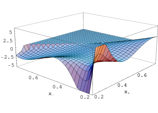
Figure 2: Function $100\cdot F^{\left(2\mu\right)}\left(x_{+},x_{-}\right)$ (see (10)) dependence of $x_{+}$ and $x_{-}$.

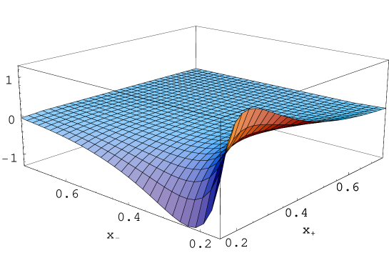
Figure 3: Function $F^{\left(2\pi\right)}\left(x_{+},x_{-}\right)$ (see (12)) dependence of $x_{+}$ and $x_{-}$.

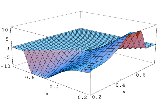
Figure 4: Function $100\cdot F^{\left(3\pi\right)}\left(x_{+},x_{-}\right)$ (see (14)) dependence of $x_{+}$ and $x_{-}$.

III Probing three current correlator in charge-odd experimental set-up of photon-proton collisions

In photon-proton collisions with production of lepton pair

$$\gamma(k)+p(p)\to e^{+}(q_{+})+e^{-}(q_{-})+X(q_{h})$$ (16)

with charge odd experimental set-up

$$\frac{d\sigma_{odd}}{d\Gamma}=\frac{1}{2}\left[F(q_{+},q_{-},q_{h})-F(q_{-},q_{+},q_{h})\right],\qquad\frac{d\sigma}{d\Gamma}=F(q_{+},q_{-},q_{h}),$$ (17)

where $d\Gamma$ is the phase volume of final particles including leptons, gives the possibility to measure the three electromagnetic currents correlator

$$H_{\mu\nu\lambda}=<p|J_{\mu}(k)J_{\nu}(q)J_{\lambda}(q_{1})|p>.$$ (18)

Really in such kind of experiment the interference of amplitudes of two mechanisms of lepton pair creation can be measured. One of them (two-photon ones) corresponds to charge-even state of lepton pair, another one (bremsstrahlung mechanism) describes the creation of a pair by the single virtual photon (see Fig. 5, a, b).

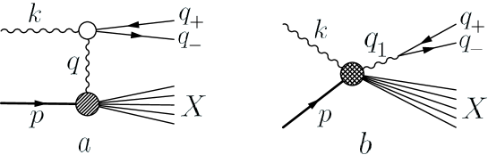
Figure 5: The two mechanisms of lepton pair creation: (a) production of lepton pair in charge-even state, (b) is the bremsstrahlung mechanism.

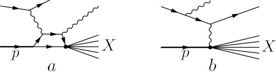
Figure 6: DVCS alternative to $\gamma p$ DIS from Fig. 5.

Charge-odd cross section can be written in form

$$\frac{d\sigma}{d\Gamma_{+}d\Gamma_{-}}\sim\frac{\alpha^{3}}{q^{2}q_{1}^{2}}L^{(e)}_{\mu\nu\lambda}H_{\mu\nu\lambda}d\Gamma_{h},$$ (19)

with $d\Gamma_{h}$ is the phase volume of the final hadron system. Leptonic tensor $L^{(e)}_{\mu\nu\lambda}$, (we neglect lepton mass)

$$L^{(e)}_{\mu\nu\lambda}=\frac{1}{4}Tr\left[\hat{q}_{-}O_{\mu\nu}\hat{q}_{+}\gamma_{\lambda}\right],$$ (20)

with

$$O_{\mu\nu}=\frac{1}{\kappa_{-}}\gamma_{\mu}(\hat{q}_{-}-\hat{k})\gamma_{\nu}+\frac{1}{\kappa_{+}}\gamma_{\nu}(-\hat{q}_{+}+\hat{k})\gamma_{\mu},\kappa_{\pm}=2kq_{\pm}$$ (21)

obey the gauge conditions $L^{(e)}_{\mu\nu\lambda}k^{\mu}=L^{(e)}_{\mu\nu\lambda}q^{\nu}=L^{(e)}_{\mu\nu\lambda}q_{1}^{\lambda}=0$ with

$$k^{2}=q_{\pm}^{2}=0,\qquad k+q=q_{1}=q_{+}+q_{-}.$$ (22)

Leptonic tensor can be written in explicitly gauge invariant form:

$$L^{(e)}_{\mu\nu\lambda} = Q_{\lambda}T^{Q}_{\mu\nu}+P_{\nu}T^{P}_{\mu\lambda}+R_{\mu}T^{R}_{\nu\lambda},$$

$$Q_{\lambda} = \frac{1}{2}\left(\frac{1}{\kappa_{+}}-\frac{1}{\kappa_{-}}\right)[\kappa_{+}\tilde{q}_{-\lambda}+s_{1}\tilde{k}_{\lambda}],$$

$$P_{\nu} = \frac{s_{1}}{2}\left(\frac{1}{\kappa_{-}}-\frac{1}{\kappa_{+}}\right)\tilde{k}_{\nu}+\frac{\kappa_{-}+\kappa_{+}}{2\kappa_{-}}\tilde{q}_{-\nu},$$

$$R_{\mu} = \frac{s_{1}}{2}\left(\frac{1}{\kappa_{-}}-\frac{1}{\kappa_{+}}\right)\tilde{k}_{\mu}-\frac{2s_{1}+\kappa_{+}+\kappa_{-}}{2\kappa_{-}}\tilde{q}_{-\mu},$$

$$\tilde{q}_{-\mu} = q_{-\mu}-\frac{q_{-}k}{q_{+}k}q_{+\mu},\qquad\tilde{k}_{\mu}=k_{\mu},$$

$$\tilde{q}_{-\nu} = q_{-\nu}-\frac{q_{-}q}{q_{+}q}q_{+\nu},\qquad\tilde{k}_{\nu}=k_{\nu}-\frac{kq}{q_{+}q}q_{+\nu},$$

$$\tilde{q}_{-\lambda} = q_{-\lambda}-\frac{q_{-}q_{1}}{q_{+}q_{1}}q_{+\lambda},\qquad\tilde{k}_{\lambda}=k_{\lambda}-\frac{kq_{1}}{q_{+}q_{1}}q_{+\lambda},$$

besides

$$T^{Q}_{\mu\nu}=\tilde{g}_{\mu\nu}+\frac{\tilde{k}_{\nu}\tilde{q}_{-\mu}}{kq};\quad T^{P}_{\mu\lambda}=\tilde{g}_{\mu\lambda}+\frac{\tilde{k}_{\lambda}\tilde{q}_{-\mu}}{kq_{1}};\quad T^{R}_{\nu\lambda}=\tilde{g}_{\nu\lambda}+\frac{\tilde{q}_{-\nu}(\tilde{q}_{-}-\tilde{k})_{\lambda}}{qq_{1}};$$ (23)

and, finally

$$\tilde{g}_{\mu\nu}=g_{\mu\nu}-\frac{k_{\nu}q_{\mu}}{kq};\quad\tilde{g}_{\mu\lambda}=g_{\mu\lambda}-\frac{k_{\lambda}q_{1\mu}}{kq_{1}};\quad\tilde{g}_{\lambda\nu}=g_{\lambda\nu}-\frac{q_{\lambda}q_{1\mu}}{qq_{1}}.$$ (24)

The form of hadronic 3-rank tensor depends on experimental conditions of detection of hadron jet particles. It won’t be touched here.

IV Conclusion

The processes with meson production mentioned above can be studied at such a facilities as HERA and HERMES. Photon-hadron interaction processes (the analog of DIS experiments) can be realized at the facilities with the high energy photon beams. The effective meson lagrangian predictions can be examined for 2 and 3 pions production for the experiments of the first class. In particular the anomaly $2\gamma\to 3\pi$ can be measured.

In hpst1 ; hpst2 ; hpst3 charge-asymmetry in $2\pi$ production at virtual photon-proton scattering was investigated in detail. There was discussed the consequences of Pomeron and Odderon characteristics measurement.

Our results concern definite process of two and three pion production at $e-p$ collisions. We obtained some concrete values of asymmetries which is presented in form of tables and plots convenient for comparison with corresponding experimental data. This values change from $10^{-4}$ % to several percents and presumably can be measured at facilities like CEBAF.

The accuracy of our results is determined by omitted terms and doesn’t exceed 10 %. The uncertainties appear from neglecting the pion final state interaction (which is small for rather large invariant masses of pion pairs) and systematical omitting of terms

$$O\left(\frac{\alpha}{\pi},\frac{\vec{q}^{2}}{s},\frac{m_{\pi}^{2}}{M^{2}},\frac{s_{1}}{s}\right)\sim O\left(0.5\%,3-4\%,2\%,3-5\%\right),$$ (25)

and the total accuracy is of order 5-7 %.

For experiments with photon hadron production the three electromagnetic currents correlations can be studied. Unfortunately these correlations are very poorly investigated in experiments as well as theoretically Ioffe:1982qb .

Our results was obtained in frames of QED with point-like mesons. In real applications we must include formfactors of pion $J_{\mu}^{2\pi}\to F_{\pi}(q_{1}^{2})(q_{+}-q_{-})_{\mu}$. Another modification is replacement of QED coupling constant used for proton-photon interaction by ones for proton-$\rho$-meson interaction: $\alpha^{4}\to\alpha^{2}(g_{\rho nn}^{2}/(4\pi))^{2}$. Besides we must take into account the resonance character of vector mesons propagators

$$\frac{1}{q_{1}^{2}}\to Re\left(\frac{1}{q_{1}^{2}-M_{\rho}^{2}+iM_{\rho}\Gamma_{\rho}}\right)=\frac{q_{1}^{2}-M_{\rho}^{2}}{\left(q_{1}^{2}-M_{\rho}^{2}\right)^{2}+M_{\rho}^{2}\Gamma_{\rho}},$$ (26)

for $\gamma^{*}\to\rho\to 2\pi$ and the similar expression with replacement $M_{\rho},\Gamma_{\rho}\to M_{\omega},\Gamma_{\omega}$ for $\gamma^{*}\to\omega\to 3\pi$ case. All these factors was not included in calculation of spectra given above.

C-odd effects in two pions production in proton fragmentation region provides besides the possibility to measure the deviation from point pion approximation used above. Really the subprocess of two charged pions production at two photons collision for the case when one of the is real and another is virtual

$$\gamma(q)+\gamma^{*}(q_{2})\to\pi(q_{-})+\pi(q_{+})$$ (27)

can be described in terms of three kinematical singularities free amplitudes Arbuzov:1997je :

$$T^{\pi_{-}\pi_{+}}_{\rho\sigma} = a_{1}L^{(1)}_{\rho\sigma}+a_{2}L^{(2)}_{\rho\sigma}+a_{3}L^{(3)}_{\rho\sigma},$$ (28)

$$L^{(1)}_{\rho\sigma} = (qq_{2})g_{\rho\sigma}-q_{2\sigma}q_{\rho},$$

$$L^{(2)}_{\rho\sigma} = -(qq_{2})Q_{\rho}Q_{\sigma}+(qQ)(q_{2\sigma}Q_{\rho}-q_{\rho}Q_{\sigma})+(qQ)^{2}g_{\rho\sigma},$$

$$L^{(3)}_{\rho\sigma} = (qQ)(q_{2}^{2}g_{\rho\sigma}-q_{2\rho}q_{2\sigma})+Q_{\sigma}((qq_{2})q_{2\rho}-q_{2}^{2}q_{\rho}),$$

with $Q=(q_{+}-q_{-})/2$. All three tensor structures are gauge invariant

$$L^{(i)}_{\rho\sigma}q^{\sigma}=L^{(i)}_{\rho\sigma}q_{2}^{\rho}=0.$$ (29)

The case of point-like pions corresponds to the choice

$$a^{(1)}_{0}=\frac{-1}{\chi_{+}+\chi_{-}}\left(\frac{\chi_{+}}{\chi_{-}}+\frac{\chi_{-}}{\chi_{+}}\right),\qquad a^{(2)}_{0}=\frac{4}{\chi_{+}\chi_{-}},\qquad a^{(3)}_{0}=0,$$ (30)

where $2qQ=\chi_{+}-\chi_{-}$, $qq_{2}=\chi_{+}+\chi_{-}$, $\chi_{\pm}=qq_{\pm}$. We note that in charge-odd experimental set-up differential cross section contains the linear combination of amplitudes.

Photon-proton deep inelastic interaction (see Section III) can be considered as an alternative to deep inelastic Compton scattering (see Fig. 6, a, b) where as well three current correlator $H_{\mu\nu\lambda}$ can be measured DVCS .

Appendix A Sudakov’s parametrization

For light lepton-proton scattering $e(p_{1})+p(p)\to e(p_{1}^{\prime})+q(q_{-})+\bar{q}(q_{+})+\cdots+p(p^{\prime})$ in high energy limit (keeping in mind the experimental requirement of detecting the final state particles i.e. we must imply the polar angles between their 3-momenta and the beam axes to be sufficiently large) we can consider the leptons ($e^{\pm},\mu^{\pm}$) as well as pions $\pi^{+,-,0}$ to be massless. Errors caused by this assumptions is of order

$$O\left(\left(\frac{m_{\pi}}{M}\right)^{2},\frac{m_{\pi}^{2}}{s_{1}},\frac{s_{1}}{s}\right),$$ (31)

with $m_{\pi}$, $M$ are masses of pion and proton, $s_{1}$-invariant mass square of produced particles (excluding the scattered electron), $s=2pp_{1}\gg s_{1}\sim M^{2}$.

Introducing the light-like 4-vector $\tilde{p}=p-p_{1}(M^{2}/s)$ we use the standard Sudakov parametrization of 4-momenta of problem:

$$q_{i}=x_{i}\tilde{p}+\beta_{i}p_{1}+q_{i\bot},\qquad a_{\bot}p_{1}=a_{\bot}p=0,\qquad\tilde{p}^{2}=p_{1}^{2}=0,$$

$$p^{\prime}=\Delta\tilde{p}+\beta_{p}p_{1}+p^{\prime}_{\bot},\qquad q^{2}=q_{\bot}^{2}=-\vec{q}^{2},\qquad p=\tilde{p}+\frac{M^{2}}{s}p_{1},$$

$$q=p_{1}-p_{1}^{\prime}=\alpha_{q}\tilde{p}+\beta_{q}p_{1}+q_{\bot}.$$ (32)

We imply $\vec{q}_{i}$ to be two-dimensional vectors situated in the plane transversal to the initial electron direction of motion (chosen as a z-axes direction).

Putting on the mass shell conditions $q_{i}^{2}=0$, $(p^{\prime})^{2}=M^{2}$, permits to exclude the ”small” coefficients $\beta_{i}$:

$$\beta_{i}=\frac{\vec{q}_{i}^{2}}{sx_{i}},\qquad\beta_{p}=\frac{(\vec{p}^{\prime}_{i})^{2}+M^{2}}{s\Delta}.$$ (33)

Both light-cone component of transfer momentum $q$, $\alpha_{q}$, $\beta_{q}$ are small (of order of $s_{1}/s$) so we have $q^{2}\approx-\vec{q}^{2}$. The conservation law reads as

$$q+p = q_{+}+q_{-}+...+p^{\prime},$$

$$1 = x_{+}+x_{-}+...+\Delta,$$

$$\vec{q} = \vec{q}_{+}+\vec{q}_{-}+...+\vec{p}^{\prime},$$

$$\beta_{q}+\frac{M^{2}}{s} = \beta_{+}+\beta_{-}+...+\beta_{p}.$$

In the center-of mass of initial particles the quantities $x_{i}$-are the fractions of energy of the initial proton. Scattering angles of the set of particles, moving along initial proton direction of motion $\theta_{i}$ are small quantities $\theta_{i}=\frac{2|\vec{q}_{i}|}{x_{i}\sqrt{s}}$.

Special attention must be paid for describing the processes in the laboratory frame, with resting proton. In this frame the light-like 4-vectors are

$$\tilde{p}=\frac{M}{2}(1,-1,0,0),\qquad p_{1}=E(1,1,0,0),\qquad s=2ME.$$ (34)

Energies of pions are $E_{i}=\frac{x_{i}M}{2}+\frac{\vec{q}_{i}^{2}}{2x_{i}M}$ and the energy of the scattered proton is $E^{\prime}=\frac{\Delta M}{2}+\frac{(\vec{p}^{\prime})^{2}+M^{2}}{2M\Delta}$. The scattering angles of the pions and recoil proton are the quantities of order of unity :

$$\sin\theta_{i} = \frac{2x_{i}M|\vec{q}_{i}|}{M^{2}x_{i}^{2}+\vec{q}_{i}^{2}},$$

$$\tan\theta = \frac{2M\Delta|\vec{p}^{\prime}|}{(\vec{p}^{\prime})^{2}+M^{2}(1-\Delta^{2})}.$$

We put here the expressions of kinematical invariants entering $R_{i}$ in terms of Sudakov’s variables:

$$d_{\pm} = \left(q_{\pm}-q\right)^{2}-m^{2}=-\vec{q}^{2}+2\vec{q}_{\pm}\vec{q}-s_{1}x_{\pm},$$

$$2q_{\pm}q_{2} = 2\vec{q}_{\pm}\vec{p}^{\prime}+\frac{\vec{q}_{\pm}^{2}\bar{\Delta}}{x_{\pm}}-\frac{x_{\pm}}{\Delta}[(\vec{p}^{\prime})^{2}+\bar{\Delta}M^{2}],$$

$$2q_{\pm}q = -2\vec{q}\vec{q}_{\pm}+s_{1}x_{\pm},$$

$$2q_{+}q_{-} = \frac{(\vec{q}_{-}x_{+}-\vec{q}_{+}x_{-})^{2}}{x_{-}x_{+}},$$

$$2q_{\pm}q_{0} = \frac{(\vec{q}_{\pm}x_{0}-\vec{q}_{0}x_{\pm})^{2}}{x_{\pm}x_{0}},$$

$$q_{2}^{2}=-\frac{1}{\Delta}[(\vec{p}^{\prime})^{2}+\bar{\Delta}^{2}M^{2}],\qquad\bar{\Delta}=1-\Delta,$$

$$q_{1}^{2}=(q+q_{2})^{2}=-\vec{q}^{2}+q_{2}^{2}+2\vec{q}\vec{p}^{\prime}+s_{1}\bar{\Delta}.$$ (35)

The quantity $s_{1}$ for $\pi_{+},\pi_{-}p^{\prime}$ jet have a form

$$s_{1} = -M^{2}+\frac{\vec{q}_{+}^{2}}{x_{+}}+\frac{\vec{q}_{-}^{2}}{x_{-}}+\frac{\vec{p}^{\prime 2}+M^{2}}{\Delta},\vec{q}=\vec{q}_{+}+\vec{q}_{-}+\vec{p}^{\prime};$$ (36)

and for $\pi_{+},\pi_{-},\pi_{0}p^{\prime}$ jet is

$$s_{1} = -M^{2}+\frac{\vec{q}_{+}^{2}}{x_{+}}+\frac{\vec{q}_{-}^{2}}{x_{-}}+\frac{\vec{q}_{0}^{2}}{x_{0}}+\frac{\vec{p}^{\prime 2}+M^{2}}{\Delta},\vec{q}=\vec{q}_{+}+\vec{q}_{-}+\vec{q}_{0}+\vec{p}^{\prime}.$$ (37)

The simplified expressions for vertex functions $V^{p}_{\mu}$, $V^{m}_{\lambda}$, $I^{\pi}_{\lambda}$, $\Pi_{\lambda}$ (lowest order on $|\vec{q}|$ expression) are

$$V^{p}_{\mu} = \frac{2\vec{p}\vec{q}}{s_{10}^{2}\Delta}\gamma_{\mu}+\frac{\gamma_{\mu}\hat{q}_{\bot}\hat{p}_{1}}{ss_{10}}+\frac{\hat{p}_{1}\hat{q}_{\bot}\gamma_{\mu}}{ss_{10}\Delta},\qquad\vec{p}=\vec{q}_{+}+\vec{q}_{-},$$

$$V^{m}_{\lambda} = \frac{2\vec{q}\vec{r}}{s_{10}^{2}x_{+}x_{-}}\gamma_{\lambda}+\frac{\hat{p}_{1}\hat{q}_{\bot}\gamma_{\lambda}}{s_{1}x_{-}}-\frac{\gamma_{\lambda}\hat{q}_{\bot}\hat{p}_{1}}{s_{1}x_{+}},\qquad\vec{r}=x_{-}\vec{q}_{+}-x_{+}\vec{q}_{-},$$

$$I^{\pi}_{\nu} = \frac{1}{s_{10}}\left(\frac{2\vec{q}_{-}\vec{q}}{s_{10}x_{-}}\left(2q_{+}-q_{2}\right)_{\nu}+\frac{2\vec{q}_{+}\vec{q}}{s_{10}x_{+}}\left(2q_{-}-q_{2}\right)_{\nu}+2q^{\bot}_{\nu}\right),$$

$$\Pi^{\nu} = \frac{1}{s}\left[\rho\left(p_{1}\nu q_{\bot}q_{2}\right)-\left(p_{1}\nu q_{\bot}q_{0}\right)-\frac{q_{+}^{\nu}}{q_{+}q_{2}}\left(p_{1}q_{\bot}q_{-}q_{0}\right)-\frac{q_{-}^{\nu}}{q_{-}q_{2}}\left(p_{1}q_{\bot}q_{+}q_{0}\right)\right]-$$

$$- \frac{1}{s_{10}}\left[\frac{\vec{q}_{+}\vec{q}}{q_{+}q}\left(\nu q_{2}q_{-}q_{0}\right)+\frac{\vec{q}_{-}\vec{q}}{q_{-}q}\left(\nu q_{2}q_{+}q_{0}\right)\right],$$

with $s_{10}=s_{1}(\vec{q}=0)$.

$x_{-}/x_{+}$	0.15	0.20	0.25	0.30	0.35	0.40	0.45	0.50	0.55	0.60	0.65	0.70
0.15	0.000	8.338	5.625	2.112	0.000	-0.676	-0.370	0.446	1.399	2.222	2.734	2.821
0.20	-8.338	0.000	0.704	0.000	-0.406	-0.247	0.319	1.050	1.728	2.188	2.308	2.012
0.25	-5.625	-0.704	0.000	-0.135	-0.123	0.191	0.700	1.235	1.641	1.795	1.610	0.000
0.30	-2.112	0.000	0.135	0.000	0.064	0.350	0.741	1.094	1.282	1.207	0.000
0.35	0.000	0.406	0.123	-0.064	0.000	0.247	0.547	0.769	0.805	0.569
0.40	0.676	0.247	-0.191	-0.350	-0.247	0.000	0.256	0.402	0.341
0.45	0.370	-0.319	-0.700	-0.741	-0.547	-0.256	0.000	0.114
0.50	-0.446	-1.050	-1.235	-1.094	-0.769	-0.402	-0.114
0.55	-1.399	-1.728	-1.641	-1.282	-0.805	-0.341
0.60	-2.222	-2.188	-1.795	-1.207	-0.569
0.65	-2.734	-2.308	-1.610	0.000
0.70	-2.821	-2.012	0.000

Table 1: The result of integration for odd part of spectrum of $2\mu$ production $100\cdot F^{\left(2\mu\right)}\left(x_{+},x_{-}\right)$ (see (10)) for the case $\vec{q}^{2}<s_{1}$.

$x_{-}/x_{+}$	0.15	0.20	0.25	0.30	0.35	0.40	0.45	0.50	0.55	0.60	0.65	0.70
0.15	0.000	1.191	1.250	1.039	0.800	0.594	0.432	0.309	0.217	0.148	0.098	0.061
0.20	-1.191	0.000	0.346	0.400	0.357	0.288	0.221	0.162	0.115	0.078	0.050	0.028
0.25	-1.250	-0.346	0.000	0.119	0.144	0.132	0.108	0.082	0.059	0.039	0.022	0.000
0.30	-1.039	-0.400	-0.119	0.000	0.044	0.054	0.049	0.039	0.028	0.017	0.000
0.35	-0.800	-0.357	-0.144	-0.044	0.000	0.016	0.020	0.017	0.011	0.005
0.40	-0.594	-0.288	-0.132	-0.054	-0.016	0.000	0.006	0.006	0.003
0.45	-0.432	-0.221	-0.108	-0.049	-0.020	-0.006	0.000	0.001
0.50	-0.309	-0.162	-0.082	-0.039	-0.017	-0.006	-0.001
0.55	-0.217	-0.115	-0.059	-0.028	-0.011	-0.003
0.60	-0.148	-0.078	-0.039	-0.017	-0.005
0.65	-0.098	-0.050	-0.022	0.000
0.70	-0.061	-0.028	0.000

Table 2: The result of integration for odd part of spectrum of $2\pi$ production $F^{\left(2\pi\right)}\left(x_{+},x_{-}\right)$ (see (12)) for the case $\vec{q}^{2}<s_{1}$.

$x_{-}/x_{+}$	0.15	0.20	0.25	0.30	0.35	0.40	0.45	0.50	0.55
0.15	0.000	1.222	1.661	3.267	5.727	8.724	11.380	12.661	10.661
0.20	-1.037	0.000	1.114	2.826	5.088	7.261	8.551	7.544
0.25	-1.736	-1.090	0.000	1.635	3.548	4.988	4.883
0.30	-3.206	-2.831	-1.645	0.000	1.642	2.424
0.35	-5.779	-5.031	-3.509	-1.628	0.000
0.40	-8.718	-7.219	-5.003	-2.399
0.45	-11.371	-8.551	-4.934
0.50	-12.675	-7.543
0.55	-10.789

Table 3: The result of numerical integration for odd part of spectrum of $3\pi$ production $100\cdot F^{\left(3\pi\right)}\left(x_{+},x_{-}\right)$ (see (14)) for the case $\vec{q}^{2}<s_{1}$.

References

(1)
A. P. Bukhvostov, S. I. Kruglov and E. A. Kuraev,
XXVI Winter school LIYAF;
E. Witten,
Nucl. Phys. B 223, 422 (1983).
J. Wess and B. Zumino,
Phys. Lett. B 37, 95 (1971).
O. Kaymakcalan, S. Rajeev and J. Schechter,
Phys. Rev. D 30, 594 (1984).
(2)
P. Hagler, B. Pire, L. Szymanowski and O. V. Teryaev, Eur. Phys.
J. C 26 (2002) 261, [hep-ph/0207224].
(3)
P. Hagler, B. Pire, L. Szymanowski and O. V. Teryaev, Nucl. Phys.
A 711 (2002) 232, [hep-ph/0206270].
(4)
P. Hagler, B. Pire, L. Szymanowski and O. V. Teryaev, Phys. Lett. B 535 (2002) 117, [Erratum-ibid. B 540 (2002)
324], [hep-ph/0202231].
(5)
E. A. Kuraev, L. N. Lipatov, N. P. Merenkov and M. I. Strikman,
Yad. Fiz. 23, 163 (1976).
(6)
S. Mikhailov, private communication;
B. L. Ioffe and A. V. Smilga,
Nucl. Phys. B 216, 373 (1983).
(7)
A. B. Arbuzov, V. A. Astakhov, A. V. Fedorov, G. V. Fedotovich, E. A. Kuraev and N. P. Merenkov,
JHEP 9710, 006 (1997)
[arXiv:hep-ph/9703456].
(8)
E. Vinokurov and E. Kuraev, JETP 63, (1972), 1142.
(9)
A. V. Radyushkin,
Phys. Lett. B 380, 417 (1996)
[arXiv:hep-ph/9604317].