Abstract

In this article, we analyze the vertices $D^{*}D_{s}K$, $D^{*}_{s}DK$, $D_{0}D_{s}K$ and $D_{s0}DK$ within the framework of the light-cone QCD sum rules approach in an unified way. The strong coupling constants $G_{D^{*}D_{s}K}$ and $G_{D^{*}_{s}DK}$ are important parameters in evaluating the charmonium absorption cross sections in searching for the quark-gluon plasmas, our numerical values of the $G_{D^{*}D_{s}K}$ and $G_{D^{*}_{s}DK}$ are compatible with the existing estimations although somewhat smaller, the $SU(4)$ symmetry breaking effects are very large, about $60\%$. For the charmed scalar mesons $D_{0}$ and $D_{s0}$, we take the point of view that they are the conventional $c\bar{u}$ and $c\bar{s}$ mesons respectively, and calculate the strong coupling constants $G_{D_{0}D_{s}K}$ and $G_{D_{s0}DK}$ with the vector interpolating currents. The numerical values of the scalar-$D_{s}K$ and -$DK$ coupling constants $G_{D_{0}D_{s}K}$ and $G_{D_{s0}DK}$ are compatible with the existing estimations, the large values support the hadronic dressing mechanism. Furthermore, we study the dependence of the four strong coupling constants $G_{D^{*}D_{s}K}$, $G_{D^{*}_{s}DK}$, $G_{D_{0}D_{s}K}$ and $G_{D_{s0}DK}$ on the non-perturbative parameter $a_{4}$ of the twist-2 $K$ meson light-cone distribution amplitude.

PACS numbers: 12.38.Lg; 13.25.Jx; 14.40.Cs

Key Words: Strong coupling constants, light-cone QCD sum rules

1 Introduction

The suppression of the $J/\psi$ production in relativistic heavy ion collisions maybe one of the important signatures to identify the possible phase transition to the quark-gluon plasma [1]. The dissociation of the $J/\psi$ in the quark-gluon plasma due to color screening can lead to a reduction of its production, however, the $J/\psi$ suppression maybe already present in the hadron-nucleus collisions. It is necessary to separate the absorption of the $J/\psi$ by the nucleons and by the co-mover light mesons ($\pi$, $K$, $\rho$, $\omega$, etc.) before we can make a definitive conclusion about the formation of the quark-gluon plasma. It is of great importance to understand the $J/\psi$ production and absorption mechanisms in the hadronic matter. The values of the $J/\psi$ absorption cross sections by the light hadrons are not known empirically, we have to resort to some theoretical approaches. Among existing approaches for evaluating the charmonium absorption cross sections by the light hadrons, the one-meson exchange model and the effective $SU(4)$ theory are typical [2, 3]. The detailed knowledge about the hadronic vertices or the strong coupling constants which are basic parameters in the effective Lagrangians is of great importance.

The discovery of the two strange-charmed mesons $D_{s0}$ and $D_{s1}$ with spin-parity $0^{+}$ and $1^{+}$ respectively has triggered hot debate on their nature, under-structures and whether it is necessary to introduce the exotic states [4]. The mass of the $D_{s0}$ is significantly lower than the values of the $0^{+}$ state mass from the quark models and lattice simulations [5]. The difficulties to identify the $D_{s0}$ and $D_{s1}$ states with the conventional $c\overline{s}$ mesons are rather similar to those appearing in the light scalar mesons below $1GeV$. Among the various explanations, the hadronic dressing mechanism is typical. The scalar mesons $a_{0}(980)$, $f_{0}(980)$, $D_{0}$ and $D_{s0}$ may have bare $q\overline{q}$, $\bar{c}u$ and $c\bar{s}$ kernels in the $P-$wave states with strong coupling to the nearby threshold respectively, the $S-$wave virtual intermediate hadronic states (or the virtual mesons loops) play a crucial role in the composition of those bound states (or resonances due to the masses below or above the thresholds). The hadronic dressing mechanism (or unitarized quark models) takes the point of view that the $f_{0}(980)$, $a_{0}(980)$ , $D_{0}$ and $D_{s0}$ mesons have small $q\bar{q}$, $\bar{c}u$ and $c\bar{s}$ kernels of the typical $q\bar{q}$, $c\bar{u}$ and $c\bar{s}$ mesons size respectively. The strong couplings to the virtual intermediate hadronic states (or the virtual mesons loops) may result in smaller masses than the conventional scalar $q\bar{q}$ , $c\bar{u}$ and $c\bar{s}$ mesons in the constituent quark models, enrich the pure $q\bar{q}$ , $c\bar{u}$ and $c\bar{s}$ states with other components [6, 7]. Those mesons may spend part (or most part) of their lifetime as virtual $K\bar{K}$, $D_{s}K$ and $DK$ states [6, 7]. It is interesting to study the possibility of the hadronic dressing mechanism.

In this article, we calculate the values of the strong coupling constants $G_{D^{*}D_{s}K}$, $G_{D_{s}^{*}DK}$, $G_{D_{0}D_{s}K}$ and $G_{D_{s0}DK}$ within the framework of the light-cone QCD sum rules approach. The light-cone QCD sum rules approach carries out the operator product expansion near the light-cone $x^{2}\approx 0$ instead of the short distance $x\approx 0$ while the non-perturbative matrix elements are parameterized by the light-cone distribution amplitudes which classified according to their twists instead of the vacuum condensates [8, 9]. Furthermore, we study the dependence of the strong coupling constants $G_{D^{*}D_{s}K}$, $G_{D_{s}^{*}DK}$, $G_{D_{0}D_{s}K}$ and $G_{D_{s0}DK}$ on the coefficient $a_{4}$ of the twist-2 $K$ meson light-cone distribution amplitude $\phi_{K}(u)$, and estimate the values of the non-perturbative parameter. It is very difficult to determine the $a_{4}$ with the QCD sum rules, the values of the $a_{4}$ suffer from large uncertainties, as it concerns high dimension vacuum condensates which are known poorly [8, 9, 10, 11, 12]. It is of great importance to determine the values directly from the experimental data.

The article is arranged as: in Section 2, we derive the strong coupling constants $G_{D^{*}D_{s}K}$, $G_{D^{*}_{s}DK}$, $G_{D_{0}D_{s}K}$ and $G_{D_{s0}DK}$ within the framework of the light-cone QCD sum rules approach; in Section 3, the numerical results and discussions; and in Section 4, conclusion.

2 Strong coupling constants $G_{D^{*}D_{s}K}$, $G_{D^{*}_{s}DK}$, $G_{D_{0}D_{s}K}$ and $G_{D_{s0}DK}$ with light-cone QCD sum rules

In the following, we write down the definitions for the strong coupling constants $G_{D^{*}D_{s}K}$, $G_{D^{*}_{s}DK}$, $G_{D_{0}D_{s}K}$ and $G_{D_{s0}DK}$ ,

$$\langle D^{*}(q+P)D_{s}(q)|K(P)\rangle = G_{D^{*}D_{s}K}(P-q)\cdot\epsilon\,,$$

$$\langle D^{*}_{s}(q+P)D(q)|K(P)\rangle = G_{D^{*}_{s}DK}(P-q)\cdot\epsilon\,,$$

$$\langle D_{0}(q+P)D_{s}(q)|K(P)\rangle = G_{D_{0}D_{s}K}\,,$$

$$\langle D_{s0}(q+P)D(q)|K(P)\rangle = G_{D_{s0}DK}\,,$$ (1)

here the $\epsilon_{\mu}$ are the polarization vectors of the mesons $D^{*}$ and $D^{*}_{s}$. We study the strong coupling constants $G_{D^{*}D_{s}K}$, $G_{D^{*}_{s}DK}$, $G_{D_{0}D_{s}K}$ and $G_{D_{s0}DK}$ with the interpolating currents $J_{D_{s}}(x)$, $J_{D}(x)$, $J^{D_{s}}_{\mu}(x)$ and $J^{D}_{\mu}(x)$ in an unified way, and choose the two-point correlation functions $\Pi_{\mu}^{1}(P,q)$ and $\Pi_{\mu}^{2}(P,q)$,

$$\Pi_{\mu}^{1}(P,q) = i\int d^{4}x\,e^{-iq\cdot x}\,\langle 0|T\left\{J^{D}_{\mu}(0)J_{D_{s}}(x)\right\}|K(P)\rangle\,,$$ (2)

$$\Pi_{\mu}^{2}(P,q) = i\int d^{4}x\,e^{-iq\cdot x}\,\langle 0|T\left\{J^{D_{s}}_{\mu}(0)J_{D}(x)\right\}|K(P)\rangle\,,$$ (3)

$$J^{D}_{\mu}(x) = {\bar{u}}(x)\gamma_{\mu}c(x)\,,$$

$$J^{D_{s}}_{\mu}(x) = {\bar{s}}(x)\gamma_{\mu}c(x)\,,$$

$$J_{D}(x) = \bar{c}(x)i\gamma_{5}u(x)\,,$$

$$J_{D_{s}}(x) = \bar{c}(x)i\gamma_{5}s(x)\,.$$ (4)

The correlation functions $\Pi^{1(2)}_{\mu}(P,q)$ can be decomposed as

$$\Pi^{1(2)}_{\mu}(P,q) = \Pi^{1(2)}_{P}\left(q^{2},(q+P)^{2}\right)P_{\mu}+\Pi^{1(2)}_{q}\left(q^{2},(q+P)^{2}\right)q_{\mu},$$ (5)

due to the Lorentz covariance. In this article, we derive the sum rules with the tensor structures $P_{\mu}$ and $q_{\mu}$ respectively, and make detailed studies.

According to the basic assumption of current-hadron duality in the QCD sum rules approach [13], we can insert a complete series of intermediate states with the same quantum numbers as the current operators $J_{D_{s}}(x)$ ($J_{D}(x)$) and $J^{D}_{\mu}(x)$ ($J^{D_{s}}_{\mu}(x)$) into the correlation function $\Pi^{1}_{\mu}$ ($\Pi^{2}_{\mu}$) to obtain the hadronic representation. After isolating the ground states and the first orbital excited states contributions from the pole terms of the $D_{s}$, $D^{*}$ and $D_{0}$ ($D$, $D^{*}_{s}$ and $D_{s0}$ ) mesons, the correlation function $\Pi^{1}_{\mu}$ ($\Pi^{2}_{\mu}$) can be expressed in terms of the strong coupling constants $G$ and the decay constants $f_{M}$ of the heavy mesons, the explicit expressions are presented in the appendix. We use the standard definitions for the decay constants $f_{M}$ ($f_{D_{s}}$, $f_{D}$, $f_{D_{s}^{*}}$, $f_{D^{*}}$, $f_{D_{s0}}$, $f_{D_{0}}$ ) of the heavy mesons,

$$\langle 0|J_{D}(0)|D(q)\rangle = \frac{f_{D}m_{D}^{2}}{m_{c}+m_{u}}\,,$$

$$\langle 0|J_{D_{s}}(0)|D_{s}(q)\rangle = \frac{f_{D_{s}}m_{D_{s}}^{2}}{m_{c}+m_{s}}\,,$$

$$\langle 0|J^{D}_{\mu}(0)|D^{*}(q)\rangle = f_{D^{*}}m_{D^{*}}\epsilon_{\mu}\,,$$

$$\langle 0|J^{D_{s}}_{\mu}(0)|D^{*}_{s}(q)\rangle = f_{D_{s}^{*}}m_{D_{s}^{*}}\epsilon_{\mu}\,,$$

$$\langle 0|J^{D}_{\mu}(0)|D_{0}(q)\rangle = f_{D_{0}}q_{\mu}\,,$$

$$\langle 0|J^{D_{s}}_{\mu}(0)|D_{s0}(q)\rangle = f_{D_{s0}}q_{\mu}\,.$$ (6)

The quarks $c$ and $s$ have finite and non-equal masses, the non-conservation of the vector currents $J^{D_{s}}_{\mu}(x)$ and $J^{D}_{\mu}(x)$ can lead to the non-vanishing couplings to the scalar mesons $D_{s0}$ and $D_{0}$ beside the vector mesons $D^{*}_{s}$ and $D^{*}$, we can study the properties of those mesons with the two interpolating currents $J^{D_{s}}_{\mu}(x)$ and $J^{D}_{\mu}(x)$ in an unified way. Here we have not shown the contributions from the high resonances and continuum states explicitly as they are suppressed due to the double Borel transformation. The numerical values of the fractions

$$\frac{m_{D^{*}}^{2}-m_{D_{s}}^{2}+m_{K}^{2}}{m_{D^{*}}^{2}}\,,\,\frac{m_{D^{*}_{s}}^{2}-m_{D}^{2}+m_{K}^{2}}{m_{D^{*}_{s}}^{2}}$$

are less than $30\%$ and the corresponding spectral densities for the ground states are greatly suppressed, the tensor structures with $q_{\mu}$ are especially suitable for studying the first orbital excited states $D_{0}$ and $D_{s0}$ with the vector currents. The numerical values of the fractions

$$\frac{m_{D^{*}}^{2}+m_{D_{s}}^{2}-m_{K}^{2}}{m_{D^{*}}^{2}}\,,\,\frac{m_{D^{*}_{s}}^{2}+m_{D}^{2}-m_{K}^{2}}{m_{D^{*}_{s}}^{2}}$$

are about $2$, the tensor structures with $P_{\mu}$ are especially suitable for studying the ground states $D^{*}$ and $D^{*}_{s}$ with the vector currents.

Now we carry out the operator product expansion near the light-cone $x^{2}\approx 0$ to obtain the representation at the level of quark-gluon degrees of freedom for the correlation functions $\Pi^{1}_{\mu}$ and $\Pi^{2}_{\mu}$. In the following, we briefly outline the operator product expansion for the correlation functions $\Pi^{1}_{\mu}$ and $\Pi^{2}_{\mu}$ in perturbative QCD theory. The calculations are performed at the large space-like momentum regions $(q+P)^{2}\ll 0$ and $q^{2}\ll 0$, which correspond to the small light-cone distance $x^{2}\approx 0$ required by the validity of the operator product expansion approach. We write down the propagator of a massive quark in the external gluon field in the Fock-Schwinger gauge firstly [10],

$$\langle 0|T\{q_{i}(x_{1})\,\bar{q}_{j}(x_{2})\}|0\rangle=i\int\frac{d^{4}k}{(2\pi)^{4}}e^{-ik(x_{1}-x_{2})}$$

$$\left\{\frac{\not\!k+m}{k^{2}-m^{2}}\delta_{ij}-\int\limits_{0}^{1}dv\,g_{s}\,G^{\mu\nu}_{ij}(vx_{1}+(1-v)x_{2})\right.$$

$$\left.\Big{[}\frac{1}{2}\frac{\not\!k+m}{(k^{2}-m^{2})^{2}}\sigma_{\mu\nu}-\frac{1}{k^{2}-m^{2}}v(x_{1}-x_{2})_{\mu}\gamma_{\nu}\Big{]}\right\}\,,$$ (7)

here $G^{\mu\nu}$ is the gluonic field strength, $g_{s}$ denotes the strong coupling constant. Substituting the above $c$ quark propagator and the corresponding $K$ meson light-cone distribution amplitudes into the correlation functions $\Pi^{1}_{\mu}$ and $\Pi^{2}_{\mu}$ in Eqs.(2-3) and completing the integrals over the variables $x$ and $k$, finally we obtain the representation at the level of quark-gluon degrees of freedom, the explicit expressions are presented in the appendix. In calculation, we have used the two-particle and three-particle $K$ meson light-cone distribution amplitudes [8, 9, 10, 11, 12], the explicit expressions are also presented in the appendix. The parameters in the light-cone distribution amplitudes are scale dependent and can be estimated with the QCD sum rules approach [8, 9, 10, 11, 12]. In this article, the energy scale $\mu$ is chosen to be $\mu=1GeV$.

We perform the double Borel transformation with respect to the variables $Q_{1}^{2}=-(q+P)^{2}$ and $Q_{2}^{2}=-q^{2}$ for the correlation functions $\Pi_{P}^{1(2)}$ and $\Pi_{q}^{1(2)}$, and obtain the analytical expressions for those invariant functions, the explicit expressions are presented in the appendix.

In order to match the duality regions below the thresholds $s_{0}$ and $s_{0}^{\prime}$ for the interpolating currents $J^{D}_{\mu}(x)$($J^{D_{s}}_{\mu}(x)$) and $J_{D_{s}}(x)$ ($J_{D}(x)$ ) respectively, we can express the correlation functions $\Pi_{P}^{1(2)}$ and $\Pi_{q}^{1(2)}$ at the level of quark-gluon degrees of freedom into the following form,

$$\Pi_{P(q)}^{1(2)}(q^{2},(q+P)^{2}) = \int ds\int ds^{\prime}\frac{\rho(s,s^{\prime})}{\left\{s-(q+P)^{2}\right\}(s^{\prime}-q^{2})}\,,$$ (8)

then we perform the double Borel transformation with respect to the variables $Q_{1}^{2}=-(q+P)^{2}$ and $Q_{2}=-q^{2}$ directly. However, the analytical expressions for the spectral densities $\rho(s,s^{\prime})$ are hard to obtain, we have to resort to some approximations. As the contributions from the higher twist terms are suppressed by more powers of $\frac{1}{-q^{2}}$ or $\frac{1}{-(q+P)^{2}}$, the continuum subtractions will not affect the results remarkably, here we will use the expressions in Eqs.(28-29) for the three-particle (quark-antiquark-gluon) twist-3, twist-4 terms, and the two-particle twist-4 terms. In fact, their contributions are of minor importance, the dominating contributions come from the two-particle twist-2 and twist-3 terms involving the $\phi_{K}(u)$, $\phi_{p}(u)$ and $\phi_{\sigma}(u)$. We perform the same trick as Refs.[10, 14] and expand the amplitudes $\phi_{K}(u)$, $\phi_{p}(u)$ and $\phi_{\sigma}(u)$ in terms of polynomials of $1-u$,

$$\phi_{K}(u),\phi_{p}(u),\phi_{\sigma}(u),\frac{d}{du}\phi_{\sigma}(u) \Longrightarrow \sum_{k=0}^{N}b_{k}(1-u)^{k}$$ (9)

$$= \sum_{k=0}^{N}b_{k}\left(\frac{s-m_{c}^{2}}{s-q^{2}}\right)^{k},$$

then introduce the variable $s^{\prime}$ and the spectral densities are obtained. After straightforward but cumbersome calculations, we can obtain the final expressions for the double Borel transformed correlation functions $\Pi_{\mu}^{1(2)}$ at the level of quark-gluon degrees of freedom below the thresholds. The masses of the charmed mesons are $M_{D^{*}}=2.012GeV$, $M_{D^{*}_{s}}=2.112GeV$, $M_{D}=1.865GeV$, $M_{D_{s}}=1.97GeV$, $M_{D_{0}}=2.40GeV$, and $M_{D_{s0}}=2.317GeV$, the ratios are $\frac{M_{D}}{M_{D}+M_{D_{s0}}}\approx 0.45$, $\frac{M_{D}}{M_{D}+M_{D^{*}_{s}}}\approx 0.47$, $\frac{M_{D_{s}}}{M_{D_{s}}+M_{D^{*}}}\approx 0.49$ and $\frac{M_{D_{s}}}{M_{D_{s}}+M_{D_{0}}}\approx 0.45$ [15]. There exist overlapping working windows for the two Borel parameters $M_{1}^{2}$ and $M_{2}^{2}$. It’s convenient to take the value $M_{1}^{2}=M_{2}^{2}$, $u_{0}=\frac{M_{1}^{2}}{M_{1}^{2}+M_{2}^{2}}=\frac{1}{2}$, $M^{2}=\frac{M_{1}^{2}M_{2}^{2}}{M_{1}^{2}+M_{2}^{2}}=\frac{1}{2}M_{1}^{2}$, furthermore, the $K$ meson light-cone distribution amplitudes are known quite well at the value $u_{0}=\frac{1}{2}$ comparing with the values at the end-points. We can introduce the threshold parameter $s_{0}$ and make the simple replacement,

$$\exp\left\{-\frac{m_{c}^{2}+u_{0}(1-u_{0})m_{K}^{2}}{M^{2}}\right\}\rightarrow\exp\left\{-\frac{m_{c}^{2}+u_{0}(1-u_{0})m_{K}^{2}}{M^{2}}\right\}-\exp\left\{-\frac{s_{0}}{M^{2}}\right\}$$

to subtract the contributions from the higher resonances and continuum states [10], finally we obtain the following sum rules,

$$-\frac{G_{D^{*}D_{s}K}m_{D^{*}}f_{D^{*}}f_{D_{s}}m_{D_{s}}^{2}}{m_{c}+m_{s}}\frac{m_{D^{*}}^{2}+m_{D_{s}}^{2}-m_{K}^{2}}{m_{D^{*}}^{2}}\exp\left\{-\frac{m_{D^{*}}^{2}}{M_{1}^{2}}-\frac{m_{D_{s}}^{2}}{M_{2}^{2}}\right\}=AA\,;$$ (10)

$$-\frac{G_{D^{*}_{s}DK}m_{D^{*}_{s}}f_{D^{*}_{s}}f_{D}m_{D}^{2}}{m_{c}+m_{u}}\frac{m_{D^{*}_{s}}^{2}+m_{D}^{2}-m_{K}^{2}}{m_{D^{*}_{s}}^{2}}\exp\left\{-\frac{m_{D^{*}_{s}}^{2}}{M_{1}^{2}}-\frac{m_{D}^{2}}{M_{2}^{2}}\right\}=BB\,;$$ (11)

$$\frac{G_{D^{*}D_{s}K}m_{D^{*}}f_{D^{*}}f_{D_{s}}m_{D_{s}}^{2}}{m_{c}+m_{s}}\frac{m_{D^{*}}^{2}-m_{D_{s}}^{2}+m_{K}^{2}}{m_{D^{*}}^{2}}\exp\left\{-\frac{m_{D^{*}}^{2}}{M_{1}^{2}}-\frac{m_{D_{s}}^{2}}{M_{2}^{2}}\right\}$$

$$+\frac{G_{D_{0}D_{s}K}f_{D_{0}}f_{D_{s}}m_{D_{s}}^{2}}{m_{c}+m_{s}}\exp\left\{-\frac{m_{D_{0}}^{2}}{M_{1}^{2}}-\frac{m_{D_{s}}^{2}}{M_{2}^{2}}\right\}=CC\,;$$ (12)

$$\frac{G_{D^{*}_{s}DK}m_{D^{*}_{s}}f_{D^{*}_{s}}f_{D}m_{D}^{2}}{m_{c}+m_{u}}\frac{m_{D^{*}_{s}}^{2}-m_{D}^{2}+m_{K}^{2}}{m_{D^{*}_{s}}^{2}}\exp\left\{-\frac{m_{D^{*}_{s}}^{2}}{M_{1}^{2}}-\frac{m_{D}^{2}}{M_{2}^{2}}\right\}$$

$$+\frac{G_{D_{s0}DK}f_{D_{s0}}f_{D}m_{D}^{2}}{m_{c}+m_{u}}\exp\left\{-\frac{m_{D_{s0}}^{2}}{M_{1}^{2}}-\frac{m_{D}^{2}}{M_{2}^{2}}\right\}=DD\,;$$ (13)

$$-\frac{G_{D^{*}D_{s}K}m_{D^{*}}f_{D^{*}}f_{D_{s}}m_{D_{s}}^{2}}{m_{c}+m_{s}}\frac{m_{D^{*}}^{2}+m_{D_{s}}^{2}-m_{K}^{2}}{m_{D^{*}}^{2}}\exp\left\{-\frac{m_{D^{*}}^{2}}{M_{1}^{2}}-\frac{m_{D_{s}}^{2}}{M_{2}^{2}}\right\}$$

$$+\frac{G_{D_{0}D_{s}K}f_{D_{0}}f_{D_{s}}m_{D_{s}}^{2}}{m_{c}+m_{s}}\exp\left\{-\frac{m_{D_{0}}^{2}}{M_{1}^{2}}-\frac{m_{D_{s}}^{2}}{M_{2}^{2}}\right\}=EE\,;$$ (14)

$$-\frac{G_{D^{*}_{s}DK}m_{D^{*}_{s}}f_{D^{*}_{s}}f_{D}m_{D}^{2}}{m_{c}+m_{u}}\frac{m_{D^{*}_{s}}^{2}+m_{D}^{2}-m_{K}^{2}}{m_{D^{*}_{s}}^{2}}\exp\left\{-\frac{m_{D^{*}_{s}}^{2}}{M_{1}^{2}}-\frac{m_{D}^{2}}{M_{2}^{2}}\right\}$$

$$+\frac{G_{D_{s0}DK}f_{D_{s0}}f_{D}m_{D}^{2}}{m_{c}+m_{u}}\exp\left\{-\frac{m_{D_{s0}}^{2}}{M_{1}^{2}}-\frac{m_{D}^{2}}{M_{2}^{2}}\right\}=FF\,.$$ (15)

The explicit expressions of the notations $AA$, $BB$, $CC$, $DD$, $EE$ and $FF$ are lengthy and given explicitly in the appendix. A slight different manipulation (with the techniques taken in the Ref.[18, 19]) for the dominating contributions come from the terms involving the two-particle twist-2 and twist-3 light-cone distribution amplitudes $\phi_{K}(u)$, $\phi_{p}(u)$ and $\phi_{\sigma}(u)$ leads to the sum rules with the same type as in Ref. [19]. However, those type sum rules are not stable with respect to the variations of the Borel parameter $M^{2}$, here we will not show the expressions explicitly for simplicity. It is not surprise that the QCD sum rules as a QCD model have both advantages and shortcomings.

3 Numerical results and discussions

The input parameters are taken as $m_{s}=(140\pm 10)MeV$, $m_{c}=(1.25\pm 0.10)GeV$, $\lambda_{3}=1.6\pm 0.4$, $f_{3K}=(0.45\pm 0.15)\times 10^{-2}GeV^{2}$, $\omega_{3}=-1.2\pm 0.7$, $\omega_{4}=0.2\pm 0.1$, $a_{2}=0.25\pm 0.15$, $a_{1}=0.06\pm 0.03$ [8, 9, 10, 11, 12], $f_{K}=0.160GeV$, $m_{K}=498MeV$, $m_{D_{s0}}=2.317GeV$, $m_{D}=1.865GeV$, $m_{D_{s}}=1.97GeV$. In this article, we take the values of the $a_{4}$ to be zero, and explore the dependence of the strong coupling constants $G_{D^{*}D_{s}K}$, $G_{D^{*}_{s}DK}$, $G_{D_{0}D_{s}K}$ and $G_{D_{s0}DK}$ on this parameter.

For the threshold parameter $s^{0}_{D_{0}}$, we can use the experimental data as a guide, $m_{D_{0}}=2.40GeV$, $\Gamma_{m_{D_{0}}}=283MeV$ [15], and choose the values $s^{0}_{D_{0}}=(6.8-7.2)GeV^{2}$ to subtract the contributions from the high resonances and continuum states. The mass and width of the $D_{0}$ from Belle and Focus are $m_{D_{0}}=2308\pm 17\pm 15\pm 28MeV$, $\Gamma_{D_{0}}=276\pm 21\pm 18\pm 60MeV$ [16], $m_{D_{0}}=2407\pm 21\pm 35MeV$, $\Gamma_{D_{0}}=240\pm 55\pm 59MeV$ [17]. The predictions from the constituent quark models are $m_{D_{0}}=2.4GeV$ [5]. The values of the mass from the two collaborations have the difference about $100MeV$, in this article, we take the value $m_{D_{0}}=2.4GeV$ as input parameter, our final numerical results for the large strong coupling constant $G_{D_{0}D_{s}K}$ support smaller values for the $D_{0}$ if the same mechanism takes place for both the charmed scalar mesons $D_{0}$ and $D_{s0}$. Furthermore, the strong coupling constant $G_{D_{0}D_{s}K}$ is not sensitive to the values of the $m_{D_{0}}$, taking the values $m_{D_{0}}=2.4GeV$ or $m_{D_{0}}=2.3GeV$ can not change the conclusion qualitatively or quantitatively.

For the threshold parameters $s^{0}_{D^{*}}$, $s^{0}_{D_{s}^{*}}$ and $s^{0}_{D_{s0}}$, the experimental values of the masses are $m_{D^{*}}=2.01GeV$, $m_{D_{s}^{*}}=2.112GeV$ and $m_{D_{s0}}=2.317GeV$, the widths are very narrow [15]. We can choose the values of the threshold parameters $s^{0}_{D^{*}}=(4.7-5.1)GeV^{2}$, $s^{0}_{D_{s}^{*}}=(4.8-5.2)GeV^{2}$ and $s^{0}_{D_{s0}}=(7.0-7.4)GeV^{2}$ to subtract the contributions from the high resonances and continuum states. From Figs.1-3, we can see that the numerical values of the strong coupling constants $G_{D^{*}D_{s}K}$ and $G_{D_{0}D_{s}K}$ are not sensitive to the threshold parameters $s^{0}$ in those regions, the values we chosen here are reasonable.

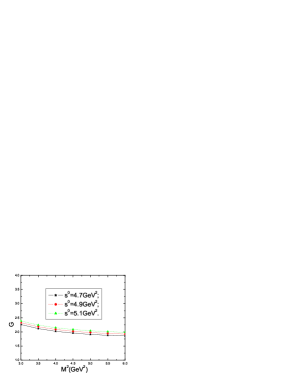
Figure 1: The $G_{D^{*}D_{s}K}$ with the parameters $M^{2}$ and $s^{0}_{D^{*}}$ from Eq.(10).

Figure 2: The $G_{D_{0}D_{s}K}$ with the parameters $M^{2}$ and $s^{0}_{D_{0}}$ from Eq.(12).

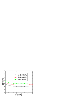
Figure 3: The $G_{D_{0}D_{s}K}$ with the parameters $M^{2}$ and $s^{0}_{D_{0}}$ from Eq.(14).

The values of the decay constants $f_{D}$, $f_{D_{s}}$, $f_{D^{*}}$, $f_{D^{*}_{s}}$, $f_{D_{0}}$ and $f_{D_{s0}}$ vary in a large range, for example, $f_{D}=(0.17\pm 0.01)GeV$, $f_{D^{*}}=(0.24\pm 0.02)GeV$ [10], $f_{D_{0}}=(0.217\pm 0.025)GeV$, $m_{D_{0}}=2.272GeV$ [20], $f_{D_{s0}}=(0.225\pm 0.025)GeV$ [21], $f_{D}=(0.177\pm 0.021)GeV$, $f_{D_{s}}=(0.205\pm 0.022)GeV$ [22], $f_{D_{0}}=(0.17\pm 0.02)GeV$ [23] from the QCD sum rules; $f_{D_{s}}=0.268GeV$, $f_{D^{*}_{s}}=0.315GeV$, $f_{D}=0.234GeV$, $f_{D^{*}}=0.310GeV$ [24], $f_{D^{*}_{s}}=0.375\pm 0.024GeV$, $f_{D^{*}}=0.340\pm 0.023GeV$ [25], $f_{D}=0.238GeV$, $f_{D_{s}}=0.241GeV$ [26] from the potential models; $f_{D^{*}_{s}}=326^{+21}_{-17}MeV$ , $f_{D^{*}}=223^{+23}_{-19}MeV$ [27] from the quark models, and $f_{D}=(222.6\pm 16.7^{+2.8}_{-3.4})MeV$ from the experimental data [28]. For a review of the values of the decay constants for the mesons $D$ and $D_{s}$ from the QCD sum rules and lattice QCD, one can consult the second article of the Ref.[9].

In this article, we take the following constraints for the decay constants,

$$1.0<\frac{f_{D_{s0}}}{f_{D_{0}}}\approx\frac{f_{D^{*}_{s}}}{f_{D^{*}}}\approx\frac{f_{D_{s}}}{f_{D}}<1.1\,,$$ (16)

and choose the values,

$$f_{D_{s}}=(0.25\pm 0.02)GeV\, \,f_{D}=(0.23\pm 0.02)GeV,$$ ,

$$f_{D_{s0}}=(0.225\pm 0.025)GeV\, \,f_{D_{0}}=(0.217\pm 0.020)GeV\,,$$ ,

$$f_{D^{*}_{s}}=(0.26\pm 0.02)GeV\, \,f_{D^{*}}=(0.24\pm 0.02)GeV\,\,.$$ , (17)

In numerical calculation, we observe that the values of the strong coupling constants $G_{D^{*}D_{s}K}$, $G_{D^{*}_{s}DK}$, $G_{D_{0}D_{s}K}$ and $G_{D_{s0}DK}$ are sensitive to the six hadronic parameters, small variations of those parameters can lead to relatively large changes for the numerical values, refining the six hadronic parameters is of great importance.

The Borel parameters in Eqs.(10-11) are taken as $M_{1}^{2}=M_{2}^{2}=(6-12)GeV^{2}$ and $M^{2}=(3-6)GeV^{2}$, in those regions, the values of the strong coupling constants $G_{D^{*}D_{s}K}$ and $G_{D^{*}_{s}DK}$ are rather stable from the sum rules in Eqs.(10-11) with the simple subtraction, which are shown, for example, in the Fig.1 and Figs.4-7 for the strong coupling constant $G_{D^{*}D_{s}K}$, similar figures can be obtained if the values of the strong coupling constant $G_{D^{*}_{s}DK}$ are plotted. In this article, we only show the numerical values from the sum rules in Eq.(10), Eq.(12) and Eq.(14) explicitly for simplicity.

The Borel parameters in Eqs.(12-15) are chosen as $M_{1}^{2}=M_{2}^{2}=(10-20)GeV^{2}$ and $M^{2}=(5-10)GeV^{2}$, in those regions, the values of the strong coupling constants $G_{D_{0}D_{s}K}$ and $G_{D_{s0}DK}$ are rather stable from the sum rules in Eqs.(12-13) with the simple subtraction, which are shown in the Fig2, Figs.4-6 and Fig.8 for an illustration. However, the strong coupling constants $G_{D_{0}D_{s}K}$ and $G_{D_{s0}DK}$ from the sum rules in Eqs.(14-15) have a negative sign comparing with the corresponding ones from the sum rules in Eqs.(12-13), and much smaller absolute values. The fractions

$$\frac{m_{D^{*}}^{2}+m_{D_{s}}^{2}-m_{K}^{2}}{m_{D^{*}}^{2}}\,,\,\frac{m_{D^{*}_{s}}^{2}+m_{D}^{2}-m_{K}^{2}}{m_{D^{*}_{s}}^{2}}$$

are about $2$. In the sum rules in Eqs.(10-11), the ground state saturate condition can be safely satisfied below the threshold $s^{0}_{D^{*}}$ ($s^{0}_{D^{*}_{s}}$). The vector interpolating current $J_{\mu}^{D}(x)$ ($J_{\mu}^{D_{s}}(x)$) has both non-vanishing couplings to the vector state $D^{*}$ ($D^{*}_{s}$) and to the scalar state $D_{0}$ ($D_{s0}$), there are two hadronic states, the ground state $D^{*}$ ($D^{*}_{s}$) and the first orbital excited state $D_{0}$ ($D_{s0}$) in the channel $\bar{c}u$ ($\bar{c}s$) below the threshold $s^{0}_{D_{0}}$ ($s^{0}_{D_{s0}}$), the ground states $D^{*}$ and $D^{*}_{s}$ are not suppressed due to the factor $2$, the sum rules in Eqs.(14-15) are not suitable for studying the strong coupling constants $G_{D_{0}D_{s}K}$ and $G_{D_{s0}DK}$, our final numerical values support this assumption. We show this fact in the Fig.3 for an illustration.

We determine the values of the strong coupling constants $G_{D^{*}D_{s}K}$ and $G_{D^{*}_{s}DK}$ from the Eq.(10) and Eq.(11) respectively, then use those values as the input parameters, and calculate the values of the strong coupling constants $G_{D_{0}D_{s}K}$ and $G_{D_{s0}DK}$ from the Eqs.(12-15) respectively.

The uncertainties of the five parameters $\omega_{4}$, $\omega_{3}$, $\lambda_{3}$, $m_{c}$ and $a_{1}$ can not lead to large uncertainties for the numerical values. The main uncertainties come from the ten parameters $f_{3K}$, $m_{s}$, $a_{2}$, $\eta_{4}$, $f_{D}$, $f_{D^{*}}$, $f_{D^{*}_{s}}$, $f_{D_{0}}$, $f_{D_{s}}$ and $f_{D_{s0}}$, small variations of those parameters can lead to relatively large changes for the numerical values, which are shown in the Figs.4-8 for an illustration.

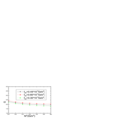
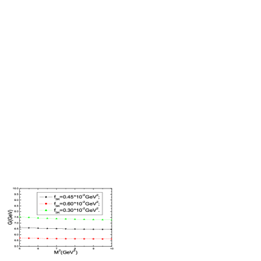
Figure 4: The $G_{D^{*}D_{s}K}$ and $G_{D_{0}D_{s}K}$ with the parameters $M^{2}$ and $f_{3K}$ from Eq.(10) and Eq.(12) respectively.

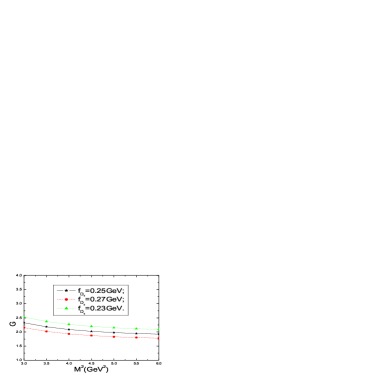
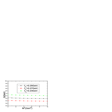
Figure 5: The $G_{D^{*}D_{s}K}$ and $G_{D_{0}D_{s}K}$ with the parameters $M^{2}$ and $f_{D_{s}}$ from Eq.(10) and Eq.(12) respectively.

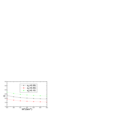
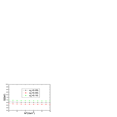
Figure 6: The $G_{D^{*}D_{s}K}$ and $G_{D_{0}D_{s}K}$ with the parameters $M^{2}$ and $a_{2}$ from Eq.(10) and Eq.(12) respectively.

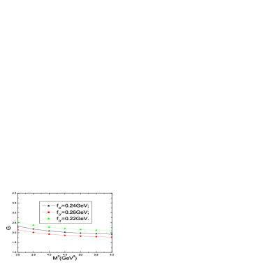
Figure 7: The $G_{D^{*}D_{s}K}$ with the parameters $M^{2}$ and $f_{D^{*}}$ from Eq.(10).

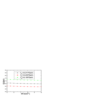
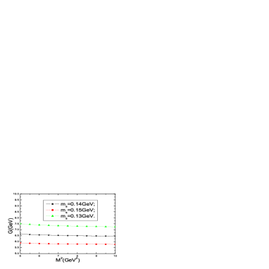
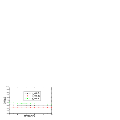
Figure 8: The $G_{D_{0}D_{s}K}$ with the parameters $M^{2}$ and $f_{D_{0}}$, $m_{s}$, $\eta_{4}$ from Eq.(12).

Taking into account all the uncertainties, finally we obtain the numerical results for the strong coupling constants,

$$G_{D^{*}D_{s}K}=2.02^{+0.84}_{-0.56}\,,\,G_{D_{0}D_{s}K}=6.5^{+1.8}_{-1.5}GeV\,,$$

$$G_{D^{*}_{s}DK}=1.84^{+0.91}_{-0.63}\,,\,G_{D_{s0}DK}=5.9^{+1.7}_{-1.6}GeV\,,$$ (18)

which are shown in the Figs.9-10 respectively.

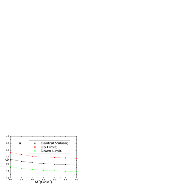
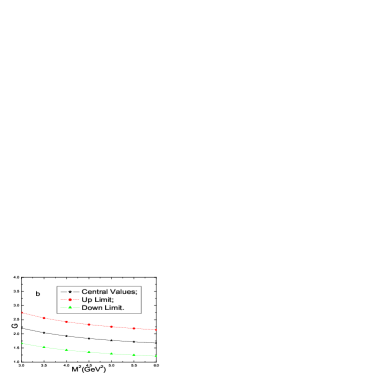
Figure 9: The $G_{D^{*}D_{s}K}$(a) and $G_{D^{*}_{s}DK}$(b) with the parameter $M^{2}$ from Eq.(10) and Eq.(11) respectively.

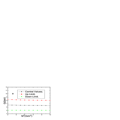
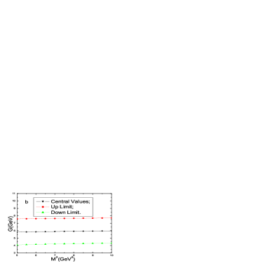
Figure 10: The $G_{D_{0}D_{s}K}$(a) and $G_{D_{s0}DK}$(b) with the parameter $M^{2}$ from Eq.(12) and Eq.(13) respectively.

The strong coupling constants $G_{D^{*}D_{s}K}$, $G_{D^{*}_{s}DK}$, $G_{D_{0}D_{s}K}$ and $G_{D_{s0}DK}$ can be related to the parameters $g$ and $h$ in the heavy-light Chiral perturbation theory [29, 39],

$$G_{SP\pi} = \sqrt{m_{S}m_{P}}\frac{m_{S}^{2}-m_{P}^{2}}{m_{S}}\frac{|h|}{f_{\pi}}\,,$$

$$G_{VP\pi} = \frac{2\sqrt{m_{P}m_{V}}}{f_{\pi}}g\,,$$

here the $S$ are the heavy scalar mesons with $0^{+}$, the $P$ are the heavy pseudoscalar mesons with $0^{-}$, the $V$ are the heavy vector mesons with $1^{-}$, and the $\pi$ stand for the light pseudoscalar mesons.

The parameter $g$ has been calculated with the light-cone QCD sum rules [32, 33, 34], the quark models [35, 36] and extracted from the experimental data [37, 38]. The values vary in a large range, the corresponding values of the strong coupling constants $G_{D^{*}D_{s}K}$ and $G_{D^{*}_{s}DK}$ in the $SU(3)$ limit for the light pseudoscalar mesons are listed in the Table.1. From the table, we can see that our numerical results are compatible with the existing estimations, although somewhat smaller.

The values of the strong coupling constants $G_{D^{*}D_{s}K}$ and $G_{D^{*}_{s}DK}$ are sensitive to the non-perturbative parameter $a_{4}$, if we take a larger value rather than zero, larger values of the $G_{D^{*}D_{s}K}$ and $G_{D^{*}_{s}DK}$ are obtained. The $G_{D^{*}D_{s}K}$ and $G_{D^{*}_{s}DK}$ are more sensitive to the $a_{4}$ comparing with the $G_{D_{0}D_{s}K}$ and $G_{D_{s0}DK}$, which are shown in the Fig.11. In fact, the largest uncertainties come from the uncertainties of the $a_{4}$, they are ideal channels to determine this parameter directly from the experimental data. Once the experimental data for the values of the strong coupling constants $G_{D^{*}D_{s}K}$ and $G_{D^{*}_{s}DK}$ are available, powerful constraints can be put on the range of the parameter $a_{4}$. If we take the values from the QCD sum rules as input parameters [31], $G_{D^{*}D_{s}K}=3.02\pm 0.14$ and $G_{D^{*}_{s}DK}=2.84\pm 0.31$, very large values of the $a_{4}$ are obtained.

The parameter $h$ has been estimated with the light-cone QCD sum rules [39], the quark models [36], Adler-Weisberger type sum rules [40], and extracted from the experimental data [41], the values are listed in the Table.2, from those values we can estimate the values of the corresponding strong coupling constants $G_{D_{0}D_{s}K}$ and $G_{D_{s0}DK}$ in the $SU(3)$ limit for the light pseudoscalar mesons. The value of the dimensionless effective coupling constant $\Gamma/k=0.46(9)$ from Lattice QCD [42] is somewhat smaller than the values extracted from the experimental data $\Gamma/k=0.73^{+28}_{-24}$, here the $\Gamma$ is the decay width and the $k$ is the decay momentum. Our numerical values $G_{D_{0}D_{s}K}=6.5^{+1.8}_{-1.5}GeV$ and $G_{D_{s0}DK}=5.9^{+1.7}_{-1.6}GeV$ are compatible with the existing estimations in Refs.[36, 39, 40, 41], although somewhat smaller comparing with the values obtained in Ref.[19] with the scalar interpolating current for the $D_{s0}$ meson, and about $2-3$ times as large as the energy scale $M_{D_{s0}}=2.317GeV$, and favor the hadronic dressing mechanism. For a short discussion about the hadronic dressing mechanism, one can consult Ref.[19], or one can consult the original literatures for the details [6, 7].

The large values of the strong coupling constants $G_{D_{0}D_{s}K}$ and $G_{D_{s0}DK}$ obviously support the hadronic dressing mechanism, the $D_{0}$ and $D_{s0}$ (just like the scalar mesons $f_{0}(980)$ and $a_{0}(980)$, see Ref.[18]) can be taken as having small scalar $c\bar{u}$ and $c\bar{s}$ kernels of typical meson size with large virtual S-wave $D_{s}K$ and $DK$ cloud respectively. In Ref.[30], the authors analyze the unitarized two-meson scattering amplitudes from the heavy-light Chiral Lagrangian, and observe that the scalar meson $D_{s0}$ appears as the bound state pole with the strong coupling constant $G_{D_{s0}DK}=10.203GeV$. Our numerical results $G_{D_{s0}DK}=5.9^{+1.7}_{-1.6}GeV$ are smaller, the values of our previously work $G_{D_{s0}DK}=9.3^{+2.7}_{-2.1}GeV$ with the scalar interpolating current are more satisfactory [19].

$|g|$	$G_{D^{*}D_{s}K}$	$G_{D^{*}_{s}DK}$	Reference
$0.38\pm 0.08$	$9.5\pm 2.0$	$9.4\pm 2.0$	[29]
	$6.04\pm 0.28$	$5.68\pm 0.62$	[31]
$0.34\pm 0.10$	$8.5\pm 2.5$	$8.4\pm 2.5$	[32]
0.28	7.0	6.9	[33]
$0.35\pm 0.10$	$8.7\pm 2.5$	$8.7\pm 2.5$	[34]
$0.50\pm 0.02$	$12.4\pm 0.5$	$12.4\pm 0.5$	[35]
$0.61$	$15.2$	$15.1$	[36]
$0.59\pm 0.07$	$14.7\pm 1.7$	$14.6\pm 1.7$	[37]
$0.27^{+0.06}_{-0.03}$	$6.7^{+1.5}_{-0.7}$	$6.7^{+1.5}_{-0.7}$	[38]
$0.16^{+0.07}_{-0.05}$	$4.04^{+1.68}_{-1.12}$	$3.68^{+1.82}_{-1.26}$	This work

Table 1: Numerical values of the parameter $g$, and the corresponding values of the strong coupling constants $G_{D^{*}D_{s}K}$ and $G_{D^{*}_{s}DK}$ in the $SU(3)$ limit. Here we have double the values of our numerical results and the ones from Ref.[31] due to the difference between the definitions for the strong coupling constants.

$|h|$	$G_{D_{0}D_{s}K}(GeV)$	$G_{D_{s0}DK}(GeV)$	Reference
$0.88^{+0.26}_{-0.20}$	$9.4^{+2.8}_{-2.1}$	$9.3^{+2.7}_{-2.1}$	[19]
		10.203	[30]
0.536	$5.7$	$5.68$	[36]
$0.52\pm 0.17$	$5.5\pm 1.8$	$5.5\pm 1.8$	[39]
$<0.93$	$<9.9$	$<9.86$	[40]
$0.57-0.74$	6.1-7.9	6.0-7.8	[41]
$0.61^{+0.17}_{-0.14}$ (or $0.56^{+0.16}_{-0.15}$)	$6.5^{+1.8}_{-1.5}$	$5.9^{+1.7}_{-1.6}$	This work

Table 2: Numerical values of the parameter $h$, and the corresponding values of the strong coupling constants $G_{D_{0}D_{s}K}$ and $G_{D_{s0}DK}$ in the $SU(3)$ limit.

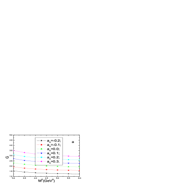
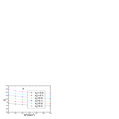
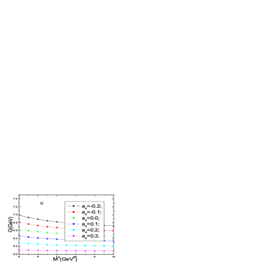
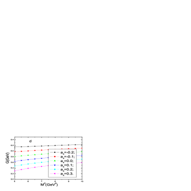
Figure 11: The $G_{D^{*}D_{s}K}$(a), $G_{D^{*}_{s}DK}$(b), $G_{D_{0}D_{s}K}$(c), $G_{D_{s0}DK}$(d) with the parameters $M^{2}$ and $a_{4}$ from Eq.(10), Eq.(11), Eq.(12), Eq.(13) respectively .

4 Conclusions

In this article, we analyze the vertices $D^{*}D_{s}K$, $D^{*}_{s}DK$, $D_{0}D_{s}K$ and $D_{s0}DK$ within the framework of the light-cone QCD sum rules approach in an unified way. The strong coupling constants $G_{D^{*}D_{s}K}$ and $G_{D^{*}_{s}DK}$ are important parameters in evaluating the charmonium absorption cross sections in searching for the quark-gluon plasmas, our numerical values of the $G_{D^{*}D_{s}K}$ and $G_{D^{*}_{s}DK}$ are compatible with the existing estimations although somewhat smaller, the $SU(4)$ symmetry breaking effects are very large, about $60\%$, the approximation of the $SU(4)$ symmetry $G_{D^{*}D_{s}K}=G_{D^{*}_{s}DK}=5.0$ is not suitable [3]. For the scalar mesons $D_{0}$ and $D_{s0}$, we take the point of view that they are the conventional $c\bar{u}$ and $c\bar{s}$ meson respectively, and calculate the strong coupling constants $G_{D_{0}D_{s}K}$ and $G_{D_{s0}DK}$ within the framework of the light-cone QCD sum rules approach. The numerical values of the scalar-$D_{s}K$ and -$DK$ coupling constants $G_{D_{0}D_{s}K}$ and $G_{D_{s0}DK}$ are compatible with the existing estimations although somewhat smaller, the large values support the hadronic dressing mechanism. Just like the scalar mesons $f_{0}(980)$ and $a_{0}(980)$, the scalar mesons $D_{0}$ and $D_{s0}$ may have small $c\bar{u}$ and $c\bar{s}$ kernels of typical $c\bar{u}$ and $c\bar{s}$ mesons size respectively. The strong coupling to virtual intermediate hadronic states (or the virtual mesons loops) can result in smaller mass than the conventional scalar mesons $c\bar{u}$ and $c\bar{s}$ in the constituent quark models, enrich the pure states $c\bar{u}$ and $c\bar{s}$ with other components. The $D_{0}$ and $D_{s0}$ may spend part (or most part) of they lifetime as virtual $D_{s}K$ and $DK$ states. Furthermore, we study the dependence of the strong coupling constants $G_{D^{*}D_{s}K}$ and $G_{D^{*}_{s}DK}$ on the non-perturbative parameter $a_{4}$ of the twist-2 $K$ meson light-cone distribution amplitude. The values of the strong coupling constants $G_{D^{*}D_{s}K}$ and $G_{D^{*}_{s}DK}$ are more sensitive to the $a_{4}$ comparing with the $G_{D_{0}D_{s}K}$ and $G_{D_{s0}DK}$. The largest uncertainties come from the uncertainties of the $a_{4}$, they are the ideal channels to determine the parameter directly from the experimental data. Once the experimental data for the values of the strong coupling constants $G_{D^{*}D_{s}K}$ and $G_{D^{*}_{s}DK}$ are available, powerful constraints can be put on the range of the parameter $a_{4}$.

Appendix

The explicit expressions of the correlation functions $\Pi^{1}_{\mu}$ and $\Pi^{2}_{\mu}$ in the hadronic representation,

$$\Pi^{1}_{\mu} = \frac{<0\mid J^{D}_{\mu}\mid D^{*}(q+P)><D^{*}D_{s}\mid K><D_{s}(q)|J_{D_{s}}\mid 0>}{\left\{m_{D^{*}}^{2}-(q+P)^{2}\right\}\left(m_{D_{s}}^{2}-q^{2}\right)}$$ (19)

$$+\frac{<0\mid J^{D}_{\mu}\mid D_{0}(q+P)><D_{0}D_{s}\mid K><D_{s}(q)|J_{D_{s}}\mid 0>}{\left\{m_{D_{0}}^{2}-(q+P)^{2}\right\}\left(m_{D_{s}}^{2}-q^{2}\right)}+\cdots$$

$$= \frac{G_{D^{*}D_{s}K}m_{D^{*}}f_{D^{*}}f_{D_{s}}m_{D_{s}}^{2}(P-q)\cdot\epsilon\epsilon_{\mu}}{\left(m_{c}+m_{s}\right)\left\{m_{D^{*}}^{2}-(q+P)^{2}\right\}\left(m_{D_{s}}^{2}-q^{2}\right)}$$

$$+\frac{G_{D_{0}D_{s}K}f_{D_{0}}f_{D_{s}}m_{D_{s}}^{2}(q+P)_{\mu}}{\left(m_{c}+m_{s}\right)\left\{m_{D_{0}}^{2}-(q+P)^{2}\right\}\left(m_{D_{s}}^{2}-q^{2}\right)}+\cdots$$

$$= \left\{\frac{G_{D^{*}D_{s}K}m_{D^{*}}f_{D^{*}}f_{D_{s}}m_{D_{s}}^{2}}{\left(m_{c}+m_{s}\right)\left\{m_{D^{*}}^{2}-(q+P)^{2}\right\}\left(m_{D_{s}}^{2}-q^{2}\right)}\frac{m_{D^{*}}^{2}-m_{D_{s}}^{2}+m_{K}^{2}}{m_{D^{*}}^{2}}\right.$$

$$\left.+\frac{G_{D_{0}D_{s}K}f_{D_{0}}f_{D_{s}}m_{D_{s}}^{2}}{\left(m_{c}+m_{s}\right)\left\{m_{D_{0}}^{2}-(q+P)^{2}\right\}\left(m_{D_{s}}^{2}-q^{2}\right)}\right\}q_{\mu}+$$

$$+\left\{-\frac{G_{D^{*}D_{s}K}m_{D^{*}}f_{D^{*}}f_{D_{s}}m_{D_{s}}^{2}}{\left(m_{c}+m_{s}\right)\left\{m_{D^{*}}^{2}-(q+P)^{2}\right\}\left(m_{D_{s}}^{2}-q^{2}\right)}\frac{m_{D^{*}}^{2}+m_{D_{s}}^{2}-m_{K}^{2}}{m_{D^{*}}^{2}}\right.$$

$$\left.+\frac{G_{D_{0}D_{s}K}f_{D_{0}}f_{D_{s}}m_{D_{s}}^{2}}{\left(m_{c}+m_{s}\right)\left\{m_{D_{0}}^{2}-(q+P)^{2}\right\}\left(m_{D_{s}}^{2}-q^{2}\right)}\right\}P_{\mu}+\cdots,$$

$$\Pi^{2}_{\mu} = \frac{<0\mid J^{D_{s}}_{\mu}\mid D_{s}^{*}(q+P)><D_{s}^{*}D\mid K><D(q)|J_{D}\mid 0>}{\left\{m_{D_{s}^{*}}^{2}-(q+P)^{2}\right\}\left(m_{D}^{2}-q^{2}\right)}$$ (20)

$$+\frac{<0\mid J^{D_{s}}_{\mu}\mid D_{s0}(q+P)><D_{s0}D\mid K><D(q)|J_{D}\mid 0>}{\left\{m_{D_{s0}}^{2}-(q+P)^{2}\right\}\left(m_{D}^{2}-q^{2}\right)}+\cdots$$

$$= \frac{G_{D_{s}^{*}DK}m_{D^{*}_{s}}f_{D^{*}_{s}}f_{D}m_{D}^{2}(P-q)\cdot\epsilon\epsilon_{\mu}}{\left(m_{c}+m_{u}\right)\left\{m_{D_{s}^{*}}^{2}-(q+P)^{2}\right\}\left(m_{D}^{2}-q^{2}\right)}$$

$$+\frac{G_{D_{s0}DK}f_{D_{s0}}f_{D}m_{D}^{2}(q+P)_{\mu}}{\left(m_{c}+m_{u}\right)\left\{m_{D_{s0}}^{2}-(q+P)^{2}\right\}\left(m_{D}^{2}-q^{2}\right)}+\cdots$$

$$= \left\{\frac{G_{D^{*}_{s}DK}m_{D^{*}_{s}}f_{D^{*}_{s}}f_{D}m_{D}^{2}}{\left(m_{c}+m_{u}\right)\left\{m_{D^{*}_{s}}^{2}-(q+P)^{2}\right\}\left(m_{D}^{2}-q^{2}\right)}\frac{m_{D^{*}_{s}}^{2}-m_{D}^{2}+m_{K}^{2}}{m_{D^{*}_{s}}^{2}}\right.$$

$$+\left.\frac{G_{D_{s0}DK}f_{D_{s0}}f_{D}m_{D}^{2}}{\left(m_{c}+m_{u}\right)\left\{m_{D_{s0}}^{2}-(q+P)^{2}\right\}\left(m_{D}^{2}-q^{2}\right)}\right\}q_{\mu}+$$

$$\left\{-\frac{G_{D^{*}_{s}DK}m_{D^{*}_{s}}f_{D^{*}_{s}}f_{D}m_{D}^{2}}{\left(m_{c}+m_{u}\right)\left\{m_{D^{*}_{s}}^{2}-(q+P)^{2}\right\}\left(m_{D}^{2}-q^{2}\right)}\frac{m_{D^{*}_{s}}^{2}+m_{D}^{2}-m_{K}^{2}}{m_{D^{*}_{s}}^{2}}\right.$$

$$+\left.\frac{G_{D_{s0}DK}f_{D_{s0}}f_{D}m_{D}^{2}}{\left(m_{c}+m_{u}\right)\left\{m_{D_{s0}}^{2}-(q+P)^{2}\right\}\left(m_{D}^{2}-q^{2}\right)}\right\}P_{\mu}+\cdots.$$

The explicit expressions of the correlation functions $\Pi^{1}_{\mu}$ and $\Pi^{2}_{\mu}$ at the level of quark-gluon degrees of freedom,

$$\Pi_{\mu}^{1} = q_{\mu}\left\{-\frac{f_{K}m_{K}^{2}}{m_{s}}\int_{0}^{1}du\frac{1}{(q+uP)^{2}-m_{c}^{2}}\left[\phi_{p}(u)-\frac{d}{6du}\phi_{\sigma}(u)\right]\right.$$

$$+m_{c}f_{K}m_{K}^{2}\int_{0}^{1}du\int_{0}^{u}dt\frac{B(t)}{\left\{(q+uP)^{2}-m_{c}^{2}\right\}^{2}}$$

$$+f_{3K}m_{K}^{2}\int_{0}^{1}dv\int_{0}^{1}d\alpha_{g}\int_{0}^{1-\alpha_{g}}d\alpha_{s}\frac{(2v-3)T(\alpha_{u},\alpha_{g},\alpha_{s})}{\left\{\left[q+((1-v)\alpha_{g}+\alpha_{s})P\right]^{2}-m_{c}^{2}\right\}^{2}}$$

$$-4m_{c}f_{K}m_{K}^{4}\int_{0}^{1}dvv\int_{0}^{1}d\alpha_{g}\int_{0}^{\alpha_{g}}d\beta\int_{0}^{1-\beta}d\alpha\frac{\Phi(1-\alpha-\beta,\beta,\alpha)}{\left\{\left[q+(1-v\alpha_{g})P\right]^{2}-m_{c}^{2}\right\}^{3}}$$

$$\left.+4m_{c}f_{K}m_{K}^{4}\int_{0}^{1}dv\int_{0}^{1}d\alpha_{g}\int_{0}^{1-\alpha_{g}}d\alpha_{s}\int_{0}^{\alpha_{s}}d\alpha\frac{\Phi(1-\alpha-\alpha_{g},\alpha_{g},\alpha)}{\left\{\left[q+((1-v)\alpha_{g}+\alpha_{s})P\right]^{2}-m_{c}^{2}\right\}^{3}}\right\}$$

$$+ P_{\mu}\left\{-\frac{f_{K}m_{K}^{2}}{m_{s}}\int_{0}^{1}du\frac{u\phi_{p}(u)}{(q+uP)^{2}-m_{c}^{2}}+m_{c}f_{K}m_{K}^{2}\int_{0}^{1}du\int_{0}^{u}dt\frac{uB(t)}{\left\{(q+uP)^{2}-m_{c}^{2}\right\}^{2}}\right.$$ (21)

$$+\frac{f_{K}m_{K}^{2}}{6m_{s}}\int_{0}^{1}\phi_{\sigma}(u)\left\{\left[1-u\frac{d}{du}\right]\frac{1}{(q+uP)^{2}-m_{c}^{2}}-\frac{2m_{c}^{2}}{\left[(q+uP)^{2}-m_{c}^{2}\right]^{2}}\right\}$$

$$+m_{c}f_{K}\int_{0}^{1}du\left\{\frac{\phi_{K}}{(q+uP)^{2}-m_{c}^{2}}-\frac{m_{K}^{2}m_{c}^{2}}{2}\frac{A(u)}{\left[(q+uP)^{2}-m_{c}^{2}\right]^{3}}\right\}$$

$$+f_{3K}m_{K}^{2}\int_{0}^{1}dv\int_{0}^{1}d\alpha_{g}\int_{0}^{1-\alpha_{g}}d\alpha_{s}\frac{\left[(1-v)\alpha_{g}+\alpha_{s}\right]\left(2v-3\right)T(\alpha_{u},\alpha_{g},\alpha_{s})}{\left\{\left[q+((1-v)\alpha_{g}+\alpha_{s})P\right]^{2}-m_{c}^{2}\right\}^{2}}$$

$$-2f_{3K}\int_{0}^{1}dvv\int_{0}^{1}d\alpha_{g}\int_{0}^{1-\alpha_{g}}d\alpha_{s}T(\alpha_{u},\alpha_{g},\alpha_{s})\frac{d}{du}\frac{1}{(q+uP)^{2}-m_{c}^{2}}\mid_{u=(1-v)\alpha_{g}+\alpha_{s}}$$

$$-4m_{c}f_{K}m_{K}^{4}\int_{0}^{1}dvv\int_{0}^{1}d\alpha_{g}\int_{0}^{\alpha_{g}}d\beta\int_{0}^{1-\beta}d\alpha\frac{(1-v\alpha_{g})\Phi(1-\alpha-\beta,\beta,\alpha)}{\left\{\left[q+(1-v\alpha_{g})P\right]^{2}-m_{c}^{2}\right\}^{3}}$$

$$+4m_{c}f_{K}m_{K}^{4}\int_{0}^{1}dv\int_{0}^{1}d\alpha_{g}\int_{0}^{1-\alpha_{g}}d\alpha_{s}\int_{0}^{\alpha_{s}}d\alpha\frac{((1-v)\alpha_{g}+\alpha_{s})\Phi(1-\alpha-\alpha_{g},\alpha_{g},\alpha)}{\left\{\left[q+((1-v)\alpha_{g}+\alpha_{s})P\right]^{2}-m_{c}^{2}\right\}^{3}}$$

$$\left.-m_{c}f_{K}m_{K}^{2}\int_{0}^{1}dv\int_{0}^{1}d\alpha_{g}\int_{0}^{1-\alpha_{g}}d\alpha_{s}\frac{\Psi(\alpha_{u},\alpha_{g},\alpha_{s})}{\left\{\left[q+((1-v)\alpha_{g}+\alpha_{s})P\right]^{2}-m_{c}^{2}\right\}^{2}}\right\}\,,$$

$$\Pi^{2}_{\mu}=\Pi^{1}_{\mu}\left(u\longleftrightarrow 1-u;\alpha_{u}\longleftrightarrow\alpha_{s}\right)\,.$$ (22)

The light-cone distribution amplitudes of the $K$ meson,

$$<0|{\bar{u}}(0)\gamma_{\mu}\gamma_{5}s(x)|K(P)> = if_{K}P_{\mu}\int_{0}^{1}due^{-iuP\cdot x}\left\{\varphi_{K}(u)+\frac{m_{K}^{2}x^{2}}{16}A(u)\right\}$$

$$+f_{K}m_{K}^{2}\frac{ix_{\mu}}{2P\cdot x}\int_{0}^{1}due^{-iuP\cdot x}B(u)\,,$$

$$<0|{\bar{u}}(0)i\gamma_{5}s(x)|K(P)> = \frac{f_{K}M_{K}^{2}}{m_{s}}\int_{0}^{1}due^{-iuP\cdot x}\varphi_{p}(u)\,,$$

$$<0|{\bar{u}}(0)\sigma_{\mu\nu}\gamma_{5}s(x)|K(P)> = i(P_{\mu}x_{\nu}-P_{\nu}x_{\mu})\frac{f_{K}M_{K}^{2}}{6m_{s}}\int_{0}^{1}due^{-iuP\cdot x}\varphi_{\sigma}(u)\,,$$

$$<0|{\bar{u}}(0)\sigma_{\alpha\beta}\gamma_{5}g_{s}G_{\mu\nu}(vx)s(x)|K(P)> = f_{3K}\left\{(P_{\mu}P_{\alpha}g^{\bot}_{\nu\beta}-P_{\nu}P_{\alpha}g^{\bot}_{\mu\beta})-(P_{\mu}P_{\beta}g^{\bot}_{\nu\alpha}\right.$$

$$\left.-P_{\nu}P_{\beta}g^{\bot}_{\mu\alpha})\right\}\int{\cal D}\alpha_{i}\varphi_{3K}(\alpha_{i})e^{-iP\cdot x(\alpha_{s}+v\alpha_{g})}\,,$$

$$<0|{\bar{u}}(0)\gamma_{\mu}\gamma_{5}g_{s}G_{\alpha\beta}(vx)s(x)|K(P)> = P_{\mu}\frac{P_{\alpha}x_{\beta}-P_{\beta}x_{\alpha}}{P\cdot x}f_{K}m_{K}^{2}$$

$$\int{\cal D}\alpha_{i}A_{\parallel}(\alpha_{i})e^{-iP\cdot x(\alpha_{s}+v\alpha_{g})}$$

$$+f_{K}m_{K}^{2}(P_{\beta}g_{\alpha\mu}-P_{\alpha}g_{\beta\mu})$$

$$\int{\cal D}\alpha_{i}A_{\perp}(\alpha_{i})e^{-iP\cdot x(\alpha_{s}+v\alpha_{g})}\,,$$

$$<0|{\bar{u}}(0)\gamma_{\mu}g_{s}\tilde{G}_{\alpha\beta}(vx)s(x)|K(P)> = P_{\mu}\frac{P_{\alpha}x_{\beta}-P_{\beta}x_{\alpha}}{P\cdot x}f_{K}m_{K}^{2}$$ (23)

$$\int{\cal D}\alpha_{i}V_{\parallel}(\alpha_{i})e^{-iP\cdot x(\alpha_{s}+v\alpha_{g})}$$

$$+f_{K}m_{K}^{2}(P_{\beta}g_{\alpha\mu}-P_{\alpha}g_{\beta\mu})$$

$$\int{\cal D}\alpha_{i}V_{\perp}(\alpha_{i})e^{-iP\cdot x(\alpha_{s}+v\alpha_{g})}\,,$$

here the operator $\tilde{G}_{\alpha\beta}$ is the dual of the $G_{\alpha\beta}$, $\tilde{G}_{\alpha\beta}={1\over 2}\epsilon_{\alpha\beta\mu\nu}G^{\mu\nu}$, ${\cal{D}}\alpha_{i}$ is defined as ${\cal{D}}\alpha_{i}=d\alpha_{1}d\alpha_{2}d\alpha_{3}\delta(1-\alpha_{1}-\alpha_{2}-\alpha_{3})$, $\Phi(\alpha_{1},\alpha_{2},\alpha_{3})=A_{\perp}+V_{\perp}+A_{\parallel}+V_{\parallel}$ and $\Psi(\alpha_{1},\alpha_{2},\alpha_{3})=A_{\parallel}+V_{\parallel}-2A_{\perp}-2V_{\perp}$. The light-cone distribution amplitudes are parameterized as

$$\phi_{K}(u,\mu) = 6u(1-u)\left\{1+a_{1}C^{\frac{3}{2}}_{1}(2u-1)+a_{2}C^{\frac{3}{2}}_{2}(2u-1)+a_{4}C^{\frac{3}{2}}_{4}(2u-1)\right\}\,,$$

$$\varphi_{p}(u,\mu) = 1+\left\{30\eta_{3}-\frac{5}{2}\rho^{2}\right\}C_{2}^{\frac{1}{2}}(2u-1)$$

$$+\left\{-3\eta_{3}\omega_{3}-\frac{27}{20}\rho^{2}-\frac{81}{10}\rho^{2}a_{2}\right\}C_{4}^{\frac{1}{2}}(2u-1)\,,$$

$$\varphi_{\sigma}(u,\mu) = 6u(1-u)\left\{1+\left[5\eta_{3}-\frac{1}{2}\eta_{3}\omega_{3}-\frac{7}{20}\rho^{2}-\frac{3}{5}\rho^{2}a_{2}\right]C_{2}^{\frac{3}{2}}(2u-1)\right\}\,,$$

$$T(\alpha_{i},\mu) = 360\alpha_{u}\alpha_{s}\alpha_{g}^{2}\left\{1+\lambda_{3}(\alpha_{u}-\alpha_{s})+\omega_{3}\frac{1}{2}(7\alpha_{g}-3)\right\}\,,$$

$$V_{\parallel}(\alpha_{i},\mu) = 120\alpha_{u}\alpha_{s}\alpha_{g}\left(v_{00}+v_{10}(3\alpha_{g}-1)\right)\,,$$

$$A_{\parallel}(\alpha_{i},\mu) = 120\alpha_{u}\alpha_{s}\alpha_{g}a_{10}(\alpha_{s}-\alpha_{u})\,,$$

$$V_{\perp}(\alpha_{i},\mu) = -30\alpha_{g}^{2}\left\{h_{00}(1-\alpha_{g})+h_{01}\left[\alpha_{g}(1-\alpha_{g})-6\alpha_{u}\alpha_{s}\right]\right.$$

$$\left.+h_{10}\left[\alpha_{g}(1-\alpha_{g})-\frac{3}{2}\left(\alpha_{u}^{2}+\alpha_{s}^{2}\right)\right]\right\}\,,$$

$$A_{\perp}(\alpha_{i},\mu) = 30\alpha_{g}^{2}(\alpha_{u}-\alpha_{s})\left\{h_{00}+h_{01}\alpha_{g}+\frac{1}{2}h_{10}(5\alpha_{g}-3)\right\},$$

$$A(u,\mu) = 6u(1-u)\left\{\frac{16}{15}+\frac{24}{35}a_{2}+20\eta_{3}+\frac{20}{9}\eta_{4}\right.$$

$$+\left[-\frac{1}{15}+\frac{1}{16}-\frac{7}{27}\eta_{3}\omega_{3}-\frac{10}{27}\eta_{4}\right]C^{\frac{3}{2}}_{2}(2u-1)$$

$$\left.+\left[-\frac{11}{210}a_{2}-\frac{4}{135}\eta_{3}\omega_{3}\right]C^{\frac{3}{2}}_{4}(2u-1)\right\}+\left\{-\frac{18}{5}a_{2}+21\eta_{4}\omega_{4}\right\}$$

$$\left\{2u^{3}(10-15u+6u^{2})\log u+2\bar{u}^{3}(10-15\bar{u}+6\bar{u}^{2})\log\bar{u}\right.$$

$$\left.+u\bar{u}(2+13u\bar{u})\right\}\,,$$

$$g_{K}(u,\mu) = 1+g_{2}C^{\frac{1}{2}}_{2}(2u-1)+g_{4}C^{\frac{1}{2}}_{4}(2u-1)\,,$$

$$B(u,\mu) = g_{K}(u,\mu)-\phi_{K}(u,\mu)\,,$$ (24)

where

$$h_{00} = v_{00}=-\frac{\eta_{4}}{3}\,,$$

$$a_{10} = \frac{21}{8}\eta_{4}\omega_{4}-\frac{9}{20}a_{2}\,,$$

$$v_{10} = \frac{21}{8}\eta_{4}\omega_{4}\,,$$

$$h_{01} = \frac{7}{4}\eta_{4}\omega_{4}-\frac{3}{20}a_{2}\,,$$

$$h_{10} = \frac{7}{2}\eta_{4}\omega_{4}+\frac{3}{20}a_{2}\,,$$

$$g_{2} = 1+\frac{18}{7}a_{2}+60\eta_{3}+\frac{20}{3}\eta_{4}\,,$$

$$g_{4} = -\frac{9}{28}a_{2}-6\eta_{3}\omega_{3}\,,$$ (25)

here $C_{2}^{\frac{1}{2}}$, $C_{4}^{\frac{1}{2}}$ and $C_{2}^{\frac{3}{2}}$ are Gegenbauer polynomials, $\eta_{3}=\frac{f_{3K}}{f_{K}}\frac{m_{q}+m_{s}}{M_{K}^{2}}$ and $\rho^{2}={m_{s}^{2}\over M_{K}^{2}}$ [8, 9, 10, 11, 12].

The explicit expressions of the Borel transformed correlation functions $B_{M}\Pi^{1}_{\mu}$ and $B_{M}\Pi^{2}_{\mu}$ in the hadronic representation,

$$B_{M}\Pi^{1}_{\mu} = \left\{\frac{G_{D^{*}D_{s}K}m_{D^{*}}f_{D^{*}}f_{D_{s}}m_{D_{s}}^{2}}{m_{c}+m_{s}}\frac{m_{D^{*}}^{2}-m_{D_{s}}^{2}+m_{K}^{2}}{m_{D^{*}}^{2}}\exp\left\{-\frac{m_{D^{*}}^{2}}{M_{1}^{2}}-\frac{m_{D_{s}}^{2}}{M_{2}^{2}}\right\}\right.$$ (26)

$$\left.+\frac{G_{D_{0}D_{s}K}f_{D_{0}}f_{D_{s}}m_{D_{s}}^{2}}{m_{c}+m_{s}}\exp\left\{-\frac{m_{D_{0}}^{2}}{M_{1}^{2}}-\frac{m_{D_{s}}^{2}}{M_{2}^{2}}\right\}\right\}q_{\mu}+$$

$$+\left\{-\frac{G_{D^{*}D_{s}K}m_{D^{*}}f_{D^{*}}f_{D_{s}}m_{D_{s}}^{2}}{m_{c}+m_{s}}\frac{m_{D^{*}}^{2}+m_{D_{s}}^{2}-m_{K}^{2}}{m_{D^{*}}^{2}}\exp\left\{-\frac{m_{D^{*}}^{2}}{M_{1}^{2}}-\frac{m_{D_{s}}^{2}}{M_{2}^{2}}\right\}\right.$$

$$\left.+\frac{G_{D_{0}D_{s}K}f_{D_{0}}f_{D_{s}}m_{D_{s}}^{2}}{m_{c}+m_{s}}\exp\left\{-\frac{m_{D_{0}}^{2}}{M_{1}^{2}}-\frac{m_{D_{s}}^{2}}{M_{2}^{2}}\right\}\right\}P_{\mu}+\cdots,$$

$$B_{M}\Pi^{2}_{\mu} = \left\{\frac{G_{D^{*}_{s}DK}m_{D^{*}_{s}}f_{D^{*}_{s}}f_{D}m_{D}^{2}}{m_{c}+m_{u}}\frac{m_{D^{*}_{s}}^{2}-m_{D}^{2}+m_{K}^{2}}{m_{D^{*}_{s}}^{2}}\exp\left\{-\frac{m_{D_{s}^{*}}^{2}}{M_{1}^{2}}-\frac{m_{D}^{2}}{M_{2}^{2}}\right\}\right.$$ (27)

$$+\left.\frac{G_{D_{s0}DK}f_{D_{s0}}f_{D}m_{D}^{2}}{m_{c}+m_{u}}\exp\left\{-\frac{m_{D_{s0}}^{2}}{M_{1}^{2}}-\frac{m_{D}^{2}}{M_{2}^{2}}\right\}\right\}q_{\mu}+$$

$$\left\{-\frac{G_{D^{*}_{s}DK}m_{D^{*}_{s}}f_{D^{*}_{s}}f_{D}m_{D}^{2}}{m_{c}+m_{u}}\frac{m_{D^{*}_{s}}^{2}+m_{D}^{2}-m_{K}^{2}}{m_{D^{*}_{s}}^{2}}\exp\left\{-\frac{m_{D_{s}^{*}}^{2}}{M_{1}^{2}}-\frac{m_{D}^{2}}{M_{2}^{2}}\right\}\right.$$

$$+\left.\frac{G_{D_{s0}DK}f_{D_{s0}}f_{D}m_{D}^{2}}{m_{c}+m_{u}}\exp\left\{-\frac{m_{D_{s0}}^{2}}{M_{1}^{2}}-\frac{m_{D}^{2}}{M_{2}^{2}}\right\}\right\}P_{\mu}+\cdots,$$

here we have not shown the contributions from the high resonances and continuum states explicitly for simplicity.

The explicit expressions of the Borel transformed correlation functions $B_{M}\Pi^{1}_{\mu}$ and $B_{M}\Pi^{2}_{\mu}$ at the level of quark-gluon degrees of freedom,

$$B_{M}\Pi_{\mu}^{1} = q_{\mu}\exp\left\{-\frac{u_{0}(1-u_{0})m_{K}^{2}+m_{c}^{2}}{M^{2}}\right\}\left\{\frac{f_{K}m_{K}^{2}M^{2}}{m_{s}}\left[\phi_{p}(u_{0})-\frac{d}{6du_{0}}\phi_{\sigma}(u_{0})\right]\right.$$ (28)

$$+m_{c}f_{K}m_{K}^{2}\int_{0}^{u_{0}}dtB(t)-f_{3K}m_{K}^{2}\int_{0}^{u_{0}}d\alpha_{s}\int_{u_{0}-\alpha_{s}}^{1-\alpha_{s}}d\alpha_{g}\frac{\left[2(\alpha_{s}-u_{0})-\alpha_{g}\right]T(\alpha_{u},\alpha_{g},\alpha_{s})}{\alpha_{g}^{2}}$$

$$-\frac{2m_{c}f_{K}m_{K}^{4}}{M^{2}}\int_{1-u_{0}}^{1}d\alpha_{g}\int_{0}^{\alpha_{g}}d\beta\int_{0}^{1-\beta}d\alpha\frac{(1-u_{0})\Phi(1-\alpha-\beta,\beta,\alpha)}{\alpha_{g}^{2}}$$

$$+\frac{2m_{c}f_{K}m_{K}^{4}}{M^{2}}\left[\int_{0}^{1-u_{0}}d\alpha_{g}\int^{u_{0}}_{u_{0}-\alpha_{g}}d\alpha_{s}\int_{0}^{\alpha_{s}}d\alpha+\int_{1-u_{0}}^{1}d\alpha_{g}\int_{u_{0}-\alpha_{g}}^{1-\alpha_{g}}d\alpha_{s}\int_{0}^{\alpha_{s}}d\alpha\right]$$

$$\left.\frac{\Phi(1-\alpha-\alpha_{g},\alpha_{g},\alpha)}{\alpha_{g}}\right\}$$

$$+ P_{\mu}\exp\left\{-\frac{u_{0}(1-u_{0})m_{K}^{2}+m_{c}^{2}}{M^{2}}\right\}\left\{\frac{f_{K}m_{K}^{2}M^{2}}{m_{s}}u_{0}\phi_{p}(u_{0})+m_{c}f_{K}m_{K}^{2}u_{0}\int_{0}^{u_{0}}dtB(t)\right.$$

$$-\frac{f_{K}m_{K}^{2}}{6m_{s}}\left[\phi_{\sigma}(u_{0})M^{2}+\frac{d}{du_{0}}u_{0}\phi_{\sigma}(u_{0})M^{2}+2m_{c}^{2}\phi_{\sigma}(u_{0})\right]$$

$$+m_{c}f_{K}\left[-\phi_{K}(u_{0})M^{2}+\frac{m_{K}^{2}m_{c}^{2}A(u_{0})}{4M^{2}}\right]$$

$$+3u_{0}f_{3K}m_{K}^{2}\int_{0}^{u_{0}}d\alpha_{s}\int_{u_{0}-\alpha_{s}}^{1-\alpha_{s}}d\alpha_{g}\frac{T(\alpha_{u},\alpha_{g},\alpha_{s})}{\alpha_{g}}$$

$$+2f_{3K}\left[M^{2}\frac{d}{du_{0}}-u_{0}m_{K}^{2}\right]\int_{0}^{u_{0}}d\alpha_{s}\int_{u_{0}-\alpha_{s}}^{1-\alpha_{s}}d\alpha_{g}\frac{\alpha_{g}+\alpha_{s}-u_{0}}{\alpha_{g}^{2}}T(\alpha_{u},\alpha_{g},\alpha_{s})$$

$$-\frac{2u_{0}m_{c}f_{K}m_{K}^{4}}{M^{2}}\int_{1-u_{0}}^{1}d\alpha_{g}\int_{0}^{\alpha_{g}}d\beta\int_{0}^{1-\beta}d\alpha\frac{(1-u_{0})\Phi(1-\alpha-\beta,\beta,\alpha)}{\alpha_{g}^{2}}$$

$$+\frac{2u_{0}m_{c}f_{K}m_{K}^{4}}{M^{2}}\left[\int_{0}^{1-u_{0}}d\alpha_{g}\int^{u_{0}}_{u_{0}-\alpha_{g}}d\alpha_{s}\int_{0}^{\alpha_{s}}d\alpha+\int_{1-u_{0}}^{1}d\alpha_{g}\int_{u_{0}-\alpha_{g}}^{1-\alpha_{g}}d\alpha_{s}\int_{0}^{\alpha_{s}}d\alpha\right]$$

$$\left.\frac{\Phi(1-\alpha-\alpha_{g},\alpha_{g},\alpha)}{\alpha_{g}}+m_{c}f_{K}m_{K}^{2}\int_{0}^{u_{0}}d\alpha_{s}\int_{u_{0}-\alpha_{s}}^{1-\alpha_{s}}d\alpha_{g}\frac{\Psi(\alpha_{u},\alpha_{g},\alpha_{s})}{\alpha_{g}}\right\}\,,$$

$$B_{M}\Pi_{\mu}^{2} = B_{M}\Pi_{\mu}^{1}(u\longleftrightarrow 1-u;\alpha_{s}\longleftrightarrow\alpha_{u})\,,$$ (29)

here $u_{0}=\frac{M_{1}^{2}}{M_{1}^{2}+M_{2}^{2}}$, $M^{2}=\frac{M_{1}^{2}M_{2}^{2}}{M_{1}^{2}+M_{2}^{2}}$.

The explicit expressions of the notations $AA$, $BB$, $CC$, $DD$, $EE$ and $FF$,

$$AA = \left\{\exp\left\{-\frac{u_{0}(1-u_{0})m_{K}^{2}+m_{c}^{2}}{M^{2}}\right\}-\exp\left\{-\frac{s^{0}_{D^{*}}}{M^{2}}\right\}\right\}\left\{\frac{f_{K}m_{K}^{2}M^{2}}{m_{s}}u_{0}\phi_{p}(u_{0})\right.$$ (30)

$$\left.-m_{c}f_{K}\phi_{K}(u_{0})M^{2}-\frac{f_{K}m_{K}^{2}}{6m_{s}}\left[\phi_{\sigma}(u_{0})M^{2}+\frac{d}{du_{0}}u_{0}\phi_{\sigma}(u_{0})M^{2}+2m_{c}^{2}\phi_{\sigma}(u_{0})\right]\right\}$$

$$+\exp\left\{-\frac{u_{0}(1-u_{0})m_{K}^{2}+m_{c}^{2}}{M^{2}}\right\}\left\{m_{c}f_{K}m_{K}^{2}u_{0}\int_{0}^{u_{0}}dtB(t)+\frac{f_{K}m_{K}^{2}m_{c}^{3}A(u_{0})}{4M^{2}}\right.$$

$$+3u_{0}f_{3K}m_{K}^{2}\int_{0}^{u_{0}}d\alpha_{s}\int_{u_{0}-\alpha_{s}}^{1-\alpha_{s}}d\alpha_{g}\frac{T(\alpha_{u},\alpha_{g},\alpha_{s})}{\alpha_{g}}$$

$$+2f_{3K}\left[M^{2}\frac{d}{du_{0}}-u_{0}m_{K}^{2}\right]\int_{0}^{u_{0}}d\alpha_{s}\int_{u_{0}-\alpha_{s}}^{1-\alpha_{s}}d\alpha_{g}\frac{\alpha_{g}+\alpha_{s}-u_{0}}{\alpha_{g}^{2}}T(\alpha_{u},\alpha_{g},\alpha_{s})$$

$$-\frac{2u_{0}m_{c}f_{K}m_{K}^{4}}{M^{2}}\int_{1-u_{0}}^{1}d\alpha_{g}\int_{0}^{\alpha_{g}}d\beta\int_{0}^{1-\beta}d\alpha\frac{(1-u_{0})\Phi(1-\alpha-\beta,\beta,\alpha)}{\alpha_{g}^{2}}$$

$$+\frac{2u_{0}m_{c}f_{K}m_{K}^{4}}{M^{2}}\left[\int_{0}^{1-u_{0}}d\alpha_{g}\int^{u_{0}}_{u_{0}-\alpha_{g}}d\alpha_{s}\int_{0}^{\alpha_{s}}d\alpha+\int_{1-u_{0}}^{1}d\alpha_{g}\int_{u_{0}-\alpha_{g}}^{1-\alpha_{g}}d\alpha_{s}\int_{0}^{\alpha_{s}}d\alpha\right]$$

$$\left.\frac{\Phi(1-\alpha-\alpha_{g},\alpha_{g},\alpha)}{\alpha_{g}}+m_{c}f_{K}m_{K}^{2}\int_{0}^{u_{0}}d\alpha_{s}\int_{u_{0}-\alpha_{s}}^{1-\alpha_{s}}d\alpha_{g}\frac{\Psi(\alpha_{u},\alpha_{g},\alpha_{s})}{\alpha_{g}}\right\}\,;$$

$$BB = \left\{\exp\left\{-\frac{u_{0}(1-u_{0})m_{K}^{2}+m_{c}^{2}}{M^{2}}\right\}-\exp\left\{-\frac{s^{0}_{D^{*}_{s}}}{M^{2}}\right\}\right\}\left\{\frac{f_{K}m_{K}^{2}M^{2}}{m_{s}}u_{0}\phi_{p}(u_{0})\right.$$

$$\left.-m_{c}f_{K}\phi_{K}(u_{0})M^{2}-\frac{f_{K}m_{K}^{2}}{6m_{s}}\left[\phi_{\sigma}(u_{0})M^{2}+\frac{d}{du_{0}}u_{0}\phi_{\sigma}(u_{0})M^{2}+2m_{c}^{2}\phi_{\sigma}(u_{0})\right]\right\}$$

$$+\exp\left\{-\frac{u_{0}(1-u_{0})m_{K}^{2}+m_{c}^{2}}{M^{2}}\right\}\left\{m_{c}f_{K}m_{K}^{2}u_{0}\int_{0}^{u_{0}}dtB(t)+\frac{f_{K}m_{K}^{2}m_{c}^{3}A(u_{0})}{4M^{2}}\right.$$

$$+3u_{0}f_{3K}m_{K}^{2}\int_{0}^{u_{0}}d\alpha_{s}\int_{u_{0}-\alpha_{s}}^{1-\alpha_{s}}d\alpha_{g}\frac{T(\alpha_{u},\alpha_{g},\alpha_{s})}{\alpha_{g}}$$

$$+2f_{3K}\left[M^{2}\frac{d}{du_{0}}-u_{0}m_{K}^{2}\right]\int_{0}^{u_{0}}d\alpha_{s}\int_{u_{0}-\alpha_{s}}^{1-\alpha_{s}}d\alpha_{g}\frac{\alpha_{g}+\alpha_{s}-u_{0}}{\alpha_{g}^{2}}T(\alpha_{u},\alpha_{g},\alpha_{s})$$

$$-\frac{2u_{0}m_{c}f_{K}m_{K}^{4}}{M^{2}}\int_{1-u_{0}}^{1}d\alpha_{g}\int_{0}^{\alpha_{g}}d\beta\int_{0}^{1-\beta}d\alpha\frac{(1-u_{0})\Phi(1-\alpha-\beta,\beta,\alpha)}{\alpha_{g}^{2}}$$

$$+\frac{2u_{0}m_{c}f_{K}m_{K}^{4}}{M^{2}}\left[\int_{0}^{1-u_{0}}d\alpha_{g}\int^{u_{0}}_{u_{0}-\alpha_{g}}d\alpha_{s}\int_{0}^{\alpha_{s}}d\alpha+\int_{1-u_{0}}^{1}d\alpha_{g}\int_{u_{0}-\alpha_{g}}^{1-\alpha_{g}}d\alpha_{s}\int_{0}^{\alpha_{s}}d\alpha\right]$$

$$\left.\frac{\Phi(1-\alpha-\alpha_{g},\alpha_{g},\alpha)}{\alpha_{g}}+m_{c}f_{K}m_{K}^{2}\int_{0}^{u_{0}}d\alpha_{s}\int_{u_{0}-\alpha_{s}}^{1-\alpha_{s}}d\alpha_{g}\frac{\Psi(\alpha_{u},\alpha_{g},\alpha_{s})}{\alpha_{g}}\right\}\mid_{\alpha_{s}\leftrightarrow\alpha_{u}}\,;$$

$$CC = \left\{\exp\left\{-\frac{u_{0}(1-u_{0})m_{K}^{2}+m_{c}^{2}}{M^{2}}\right\}-\exp\left\{-\frac{s^{0}_{D_{0}}}{M^{2}}\right\}\right\}\frac{f_{K}m_{K}^{2}M^{2}}{m_{s}}\left\{\phi_{p}(u_{0})-\frac{d}{6du_{0}}\phi_{\sigma}(u_{0})\right\}$$ (32)

$$+\exp\left\{-\frac{u_{0}(1-u_{0})m_{K}^{2}+m_{c}^{2}}{M^{2}}\right\}\left\{m_{c}f_{K}m_{K}^{2}\int_{0}^{u_{0}}dtB(t)\right.$$

$$-f_{3K}m_{K}^{2}\int_{0}^{u_{0}}d\alpha_{s}\int_{u_{0}-\alpha_{s}}^{1-\alpha_{s}}d\alpha_{g}\frac{\left[2(\alpha_{s}-u_{0})-\alpha_{g}\right]T(\alpha_{u},\alpha_{g},\alpha_{s})}{\alpha_{g}^{2}}$$

$$-\frac{2m_{c}f_{K}m_{K}^{4}}{M^{2}}\int_{1-u_{0}}^{1}d\alpha_{g}\int_{0}^{\alpha_{g}}d\beta\int_{0}^{1-\beta}d\alpha\frac{(1-u_{0})\Phi(1-\alpha-\beta,\beta,\alpha)}{\alpha_{g}^{2}}$$

$$+\frac{2m_{c}f_{K}m_{K}^{4}}{M^{2}}\left[\int_{0}^{1-u_{0}}d\alpha_{g}\int^{u_{0}}_{u_{0}-\alpha_{g}}d\alpha_{s}\int_{0}^{\alpha_{s}}d\alpha+\int_{1-u_{0}}^{1}d\alpha_{g}\int_{u_{0}-\alpha_{g}}^{1-\alpha_{g}}d\alpha_{s}\int_{0}^{\alpha_{s}}d\alpha\right]$$

$$\left.\frac{\Phi(1-\alpha-\alpha_{g},\alpha_{g},\alpha)}{\alpha_{g}}\right\}\,;$$

$$DD = \left\{\exp\left\{-\frac{u_{0}(1-u_{0})m_{K}^{2}+m_{c}^{2}}{M^{2}}\right\}-\exp\left\{-\frac{s^{0}_{D_{s0}}}{M^{2}}\right\}\right\}\frac{f_{K}m_{K}^{2}M^{2}}{m_{s}}\left\{\phi_{p}(u_{0})-\frac{d}{6du_{0}}\phi_{\sigma}(u_{0})\right\}$$ (33)

$$+\exp\left\{-\frac{u_{0}(1-u_{0})m_{K}^{2}+m_{c}^{2}}{M^{2}}\right\}\left\{m_{c}f_{K}m_{K}^{2}\int_{0}^{u_{0}}dtB(t)\right.$$

$$-f_{3K}m_{K}^{2}\int_{0}^{u_{0}}d\alpha_{s}\int_{u_{0}-\alpha_{s}}^{1-\alpha_{s}}d\alpha_{g}\frac{\left[2(\alpha_{s}-u_{0})-\alpha_{g}\right]T(\alpha_{u},\alpha_{g},\alpha_{s})}{\alpha_{g}^{2}}$$

$$-\frac{2m_{c}f_{K}m_{K}^{4}}{M^{2}}\int_{1-u_{0}}^{1}d\alpha_{g}\int_{0}^{\alpha_{g}}d\beta\int_{0}^{1-\beta}d\alpha\frac{(1-u_{0})\Phi(1-\alpha-\beta,\beta,\alpha)}{\alpha_{g}^{2}}$$

$$+\frac{2m_{c}f_{K}m_{K}^{4}}{M^{2}}\left[\int_{0}^{1-u_{0}}d\alpha_{g}\int^{u_{0}}_{u_{0}-\alpha_{g}}d\alpha_{s}\int_{0}^{\alpha_{s}}d\alpha+\int_{1-u_{0}}^{1}d\alpha_{g}\int_{u_{0}-\alpha_{g}}^{1-\alpha_{g}}d\alpha_{s}\int_{0}^{\alpha_{s}}d\alpha\right]$$

$$\left.\frac{\Phi(1-\alpha-\alpha_{g},\alpha_{g},\alpha)}{\alpha_{g}}\right\}\mid_{\alpha_{s}\leftrightarrow\alpha_{u}}\,;$$

$$EE = \left\{\exp\left\{-\frac{u_{0}(1-u_{0})m_{K}^{2}+m_{c}^{2}}{M^{2}}\right\}-\exp\left\{-\frac{s^{0}_{D_{0}}}{M^{2}}\right\}\right\}\left\{\frac{f_{K}m_{K}^{2}M^{2}}{m_{s}}u_{0}\phi_{p}(u_{0})\right.$$ (34)

$$\left.-m_{c}f_{K}\phi_{K}(u_{0})M^{2}-\frac{f_{K}m_{K}^{2}}{6m_{s}}\left[\phi_{\sigma}(u_{0})M^{2}+\frac{d}{du_{0}}u_{0}\phi_{\sigma}(u_{0})M^{2}+2m_{c}^{2}\phi_{\sigma}(u_{0})\right]\right\}$$

$$+\exp\left\{-\frac{u_{0}(1-u_{0})m_{K}^{2}+m_{c}^{2}}{M^{2}}\right\}\left\{m_{c}f_{K}m_{K}^{2}u_{0}\int_{0}^{u_{0}}dtB(t)+\frac{f_{K}m_{K}^{2}m_{c}^{3}A(u_{0})}{4M^{2}}\right.$$

$$+3u_{0}f_{3K}m_{K}^{2}\int_{0}^{u_{0}}d\alpha_{s}\int_{u_{0}-\alpha_{s}}^{1-\alpha_{s}}d\alpha_{g}\frac{T(\alpha_{u},\alpha_{g},\alpha_{s})}{\alpha_{g}}$$

$$+2f_{3K}\left[M^{2}\frac{d}{du_{0}}-u_{0}m_{K}^{2}\right]\int_{0}^{u_{0}}d\alpha_{s}\int_{u_{0}-\alpha_{s}}^{1-\alpha_{s}}d\alpha_{g}\frac{\alpha_{g}+\alpha_{s}-u_{0}}{\alpha_{g}^{2}}T(\alpha_{u},\alpha_{g},\alpha_{s})$$

$$-\frac{2u_{0}m_{c}f_{K}m_{K}^{4}}{M^{2}}\int_{1-u_{0}}^{1}d\alpha_{g}\int_{0}^{\alpha_{g}}d\beta\int_{0}^{1-\beta}d\alpha\frac{(1-u_{0})\Phi(1-\alpha-\beta,\beta,\alpha)}{\alpha_{g}^{2}}$$

$$+\frac{2u_{0}m_{c}f_{K}m_{K}^{4}}{M^{2}}\left[\int_{0}^{1-u_{0}}d\alpha_{g}\int^{u_{0}}_{u_{0}-\alpha_{g}}d\alpha_{s}\int_{0}^{\alpha_{s}}d\alpha+\int_{1-u_{0}}^{1}d\alpha_{g}\int_{u_{0}-\alpha_{g}}^{1-\alpha_{g}}d\alpha_{s}\int_{0}^{\alpha_{s}}d\alpha\right]$$

$$\left.\frac{\Phi(1-\alpha-\alpha_{g},\alpha_{g},\alpha)}{\alpha_{g}}+m_{c}f_{K}m_{K}^{2}\int_{0}^{u_{0}}d\alpha_{s}\int_{u_{0}-\alpha_{s}}^{1-\alpha_{s}}d\alpha_{g}\frac{\Psi(\alpha_{u},\alpha_{g},\alpha_{s})}{\alpha_{g}}\right\}\,;$$

$$FF = \left\{\exp\left\{-\frac{u_{0}(1-u_{0})m_{K}^{2}+m_{c}^{2}}{M^{2}}\right\}-\exp\left\{-\frac{s^{0}_{D_{s0}}}{M^{2}}\right\}\right\}\left\{\frac{f_{K}m_{K}^{2}M^{2}}{m_{s}}u_{0}\phi_{p}(u_{0})\right.$$

$$\left.-m_{c}f_{K}\phi_{K}(u_{0})M^{2}-\frac{f_{K}m_{K}^{2}}{6m_{s}}\left[\phi_{\sigma}(u_{0})M^{2}+\frac{d}{du_{0}}u_{0}\phi_{\sigma}(u_{0})M^{2}+2m_{c}^{2}\phi_{\sigma}(u_{0})\right]\right\}$$

$$+\exp\left\{-\frac{u_{0}(1-u_{0})m_{K}^{2}+m_{c}^{2}}{M^{2}}\right\}\left\{m_{c}f_{K}m_{K}^{2}u_{0}\int_{0}^{u_{0}}dtB(t)+\frac{f_{K}m_{K}^{2}m_{c}^{3}A(u_{0})}{4M^{2}}\right.$$

$$+3u_{0}f_{3K}m_{K}^{2}\int_{0}^{u_{0}}d\alpha_{s}\int_{u_{0}-\alpha_{s}}^{1-\alpha_{s}}d\alpha_{g}\frac{T(\alpha_{u},\alpha_{g},\alpha_{s})}{\alpha_{g}}$$

$$+2f_{3K}\left[M^{2}\frac{d}{du_{0}}-u_{0}m_{K}^{2}\right]\int_{0}^{u_{0}}d\alpha_{s}\int_{u_{0}-\alpha_{s}}^{1-\alpha_{s}}d\alpha_{g}\frac{\alpha_{g}+\alpha_{s}-u_{0}}{\alpha_{g}^{2}}T(\alpha_{u},\alpha_{g},\alpha_{s})$$

$$-\frac{2u_{0}m_{c}f_{K}m_{K}^{4}}{M^{2}}\int_{1-u_{0}}^{1}d\alpha_{g}\int_{0}^{\alpha_{g}}d\beta\int_{0}^{1-\beta}d\alpha\frac{(1-u_{0})\Phi(1-\alpha-\beta,\beta,\alpha)}{\alpha_{g}^{2}}$$

$$+\frac{2u_{0}m_{c}f_{K}m_{K}^{4}}{M^{2}}\left[\int_{0}^{1-u_{0}}d\alpha_{g}\int^{u_{0}}_{u_{0}-\alpha_{g}}d\alpha_{s}\int_{0}^{\alpha_{s}}d\alpha+\int_{1-u_{0}}^{1}d\alpha_{g}\int_{u_{0}-\alpha_{g}}^{1-\alpha_{g}}d\alpha_{s}\int_{0}^{\alpha_{s}}d\alpha\right]$$

$$\left.\frac{\Phi(1-\alpha-\alpha_{g},\alpha_{g},\alpha)}{\alpha_{g}}+m_{c}f_{K}m_{K}^{2}\int_{0}^{u_{0}}d\alpha_{s}\int_{u_{0}-\alpha_{s}}^{1-\alpha_{s}}d\alpha_{g}\frac{\Psi(\alpha_{u},\alpha_{g},\alpha_{s})}{\alpha_{g}}\right\}\mid_{\alpha_{s}\leftrightarrow\alpha_{u}}\,.$$

References

[1] T. Matsui, H. Satz, Phys. Lett. B178 (1986)
416; R. Vogt, Phys. Rept. 310 (1999) 197.
[2] S. G. Matinyan, B. Muller, Phys. Rev. C58 (1998)
2994; K. L. Haglin, Phys. Rev. C61 (2000) 031902; Z. W. Lin,
C. M. Ko, Phys. Rev. C62 (2000) 034903; A. Sibirtsev, K.
Tsushima, A. W. Thomas, Phys. Rev. C63 (2001) 044906.
[3] R. S. Azevedo, M. Nielsen, Phys. Rev. C69 (2004)
035201.
[4] B. Aubert et al, Phys. Rev. Lett.
90 (2003) 242001; Phys. Rev. D69 (2004) 031101;
D. Besson et al, Phys. Rev. D68 (2003)
032002; P. Krokovny et al, Phys. Rev. Lett. 91 (2003) 262002.
[5] S. Godfrey and N. Isgur, Phys. Rev. D32 (1985) 189;
S. Godfrey and R. Kokoshi, Phys. Rev. D43 (1991) 1679; G. S.
Bali, Phys. Rev. D68 (2003) 071501; A. Dougall, R. D. Kenway,
C. M. Maynard and C. Mc-Neile, Phys. Lett. B569 (2003) 41.
[6] N. A. Tornqvist, Z. Phys. C68 (1995) 647;
M. Boglione and M. R. Pennington, Phys. Rev. Lett 79 (1997)
1998; N. A. Tornqvist, hep-ph/0008136; N. A. Tornqvist and A. D.
Polosa, Nucl. Phys. A692 (2001) 259; A. Deandrea, R. Gatto, G.
Nardulli, A. D. Polosa and N. A. Tornqvist, Phys. Lett. B502
(2001) 79; F. De Fazio and M. R. Pennington, Phys. Lett. B521
(2001) 15; M. Boglione and M. R. Pennington, Phys. Rev. D65
(2002) 114010.
[7] E. van Beveren, G. Rupp, Phys. Rev. Lett. 91 (2003)
012003; D. S. Hwang, D. W. Kim , Phys. Lett. B601 (2004) 137;
Yu. A. Simonov, J. A. Tjon, Phys. Rev. D70 (2004) 114013;
E. E. Kolomeitsev, M. F. M. Lutz, Phys. Lett. B582 (2004) 39;
J. Hofmann, M. F. M. Lutz , Nucl. Phys. A733 (2004) 142.
[8]
I. I. Balitsky, V. M. Braun and A. V. Kolesnichenko, Nucl. Phys.
B312 (1989) 509; V. L. Chernyak and I. R. Zhitnitsky, Nucl.
Phys. B345 (1990) 137; V. L. Chernyak and A. R. Zhitnitsky,
Phys. Rept. 112 (1984) 173; V. M. Braun and I. E. Filyanov, Z.
Phys. C44 (1989) 157; V. M. Braun and I. E. Filyanov, Z.
Phys. C48 (1990) 239.
[9]
V. M. Braun, hep-ph/9801222; P. Colangelo and A. Khodjamirian,
hep-ph/0010175.
[10]
V. M. Belyaev, V. M. Braun, A. Khodjamirian and R. Rückl, Phys.
Rev. D51 (1995) 6177.
[11]
P. Ball, JHEP 9901 (1999) 010.
[12] P. Ball, V. M. Braun, A. Lenz, hep-ph/0603063.
[13] M. A. Shifman, A. I. and Vainshtein and V. I. Zakharov,
Nucl. Phys. B147 (1979) 385, 448; L. J. Reinders, H.
Rubinstein and S. Yazaky, Phys. Rept. 127 (1985) 1; S.
Narison, QCD Spectral Sum Rules, World Scientific Lecture Notes in
Physics 26.
[14] H. Kim, S. H. Lee and M. Oka, Prog. Theor. Phys. 109 (2003)
371.
[15] S. Eidelman et al, Phys. Lett. B592 (2004)
1.
[16] K. Abe et al, Phys. Rev. D69 (2004) 112002.
[17] J. M. Link et al, Phys. Lett. B586 (2004)
11.
[18] P. Colangelo and F. D. Fazio, Phys. Lett. B559 (2003) 49; Z. G. Wang
, W. M. Yang, S. L. Wan, Eur. Phys. J. C37 (2004) 223.
[19] Z. G. Wang, S. L. Wan, Phys. Rev. D73 (2006) 094020.
[20] S. Narison, Phys. Lett. B605 (2005) 319.
[21] P. Colangelo, F. De Fazio, A. Ozpineci, Phys. Rev. D72 (2005)
074004.
[22] J. Bordes, J. Penarrocha, K. Schilcher, JHEP 0511 (2005)
014.
[23] P. Colangelo, G. Nardulli, A. A. Ovchinnikov, N. Paver,
Phys. Lett. B269 (1991) 201.
[24] D. Ebert, R. N. Faustov, V. O. Galkin, Phys. Lett. B635 (2006)
93.
[25] G. L. Wang , Phys. Lett. B633 (2006) 492.
[26] Z. G. Wang, W. M. Yang, S. L. Wan, Nucl. Phys. A744 (2004) 156.
[27] C. Albertus, E. Hernandez, J. Nieves, J. M. Verde-Velasco,
Phys. Rev. D71 (2005) 113006.
[28] M. Artuso et al, Phys. Rev. Lett. 95 (2005)
251801; G. Bonvicini et al, Phys. Rev. D70 (2004) 112004.
[29]
R. Casalbuoni, A. Deandrea, N. Di Bartolomeo, R. Gatto, F. Feruglio,
G. Nardulli, Phys. Rept. 281 (1997) 145.
[30] F. K. Guo, P. N. Shen,
H. C. Chiang, R. G. Ping , hep-ph/0603072.
[31] M. E. Bracco, A. Cerqueira, M. Chiapparini, A. Lozea, M.
Nielsen, hep-ph/0604167.
[32] P. Colangelo, F. De Fazio,
Eur. Phys. J. C4 (1998) 503.
[33] H. C. Kim, S. H. Lee, Eur. Phys. J. C22 (2002)
707.
[34] A. Khodjamirian, R. Ruckl, S. Weinzierl, O. I. Yakovlev, Phys. Lett. B457
(1999) 245.
[35] D. Melikhov, M. Beyer, Phys. Lett. B452 (1999) 121.
[36] D. Becirevic, A. Le Yaouanc, JHEP 9903 (1999)
021.
[37] P. Colangelo, F. De Fazio, Phys. Lett. B532 (2002)
193; A. Anastassov et al, Phys. Rev. D65 (2002) 032003.
[38] I. W. Stewart, Nucl. Phys. B529 (1998) 62.
[39] P. Colangelo, F. De Fazio, G. Nardulli, N. Di Bartolomeo, R. Gatto,
Phys. Rev. D52 (1995) 6422.
[40] C. K. Chow, D. Pirjol, Phys. Rev. D54 (1996) 2063.
[41] T. Mehen, R. P. Springer, Phys. Rev. D70 (2004)
074014.
[42] C. McNeile et al, Phys. Rev. D70 (2004)
054501.