Bosonic Corrections
to The Effective Weak Mixing Angle at ${\mathcal{O}}(\alpha^{2})$

Abstract

We present the complete bosonic contributions to the effective weak mixing angle, $\sin^{2}\theta^{\mbox{\footnotesize lept}}_{\mbox{\footnotesize eff}}$, at the two-loop level in the electroweak interactions. We find their size to be about three times smaller than inferred from simple estimates from lower orders. In particular, for a Higgs boson mass, $M_{H}$, of $100$ GeV they amount to $4\times 10^{-6}$, and drop down by about an order of magnitude for $M_{H}=200$ GeV. We estimate the intrinsic error of the theory prediction of $\sin^{2}\theta^{\mbox{\footnotesize lept}}_{\mbox{\footnotesize eff}}$ to be $4.7\times 10^{-5}$.

1 Introduction

While no clear experimental evidence for the Higgs boson has been found so far, even today the Standard Model is accurately tested and the Higgs boson mass $M_{H}$ strongly constrained through precision measurements of $Z$- and $W$-boson properties. One of the most important observables in this context is the effective leptonic weak mixing angle $\sin^{2}\theta^{\mbox{\footnotesize lept}}_{\mbox{\footnotesize eff}}$. It can be defined through the vertex form factors for the vector and axial-vector interactions between the $Z$ boson and fermions $f$:

$$\sin^{2}\theta^{\mbox{\footnotesize lept}}_{\mbox{\footnotesize eff}}=\frac{1}{4}\left(1-\Re\left(\frac{g_{V}(M_{Z}^{2})}{g_{A}(M_{Z}^{2})}\right)\right).$$ (1)

with the $g_{V,A}$ the effective couplings in the vertex $i\;\overline{l}\gamma^{\mu}(g_{V}-g_{A}\gamma_{5})l\;Z_{\mu}$.

The experimental value for $\sin^{2}\theta^{\mbox{\footnotesize lept}}_{\mbox{\footnotesize eff}}$ is derived from various asymmetries measured at the $Z$ resonance pole. The precision of the current experimental value $\sin^{2}\theta^{\mbox{\footnotesize lept}}_{\mbox{\footnotesize eff}}=0.23153\pm 0.00016$ [1] could be improved by about one order of magnitude by a future linear collider experiment [2]. Since the radiative corrections to $\sin^{2}\theta^{\mbox{\footnotesize lept}}_{\mbox{\footnotesize eff}}$ depend sensitively on the value of $M_{H}$, the high experimental precision allows to put strong constraints on the Higgs boson mass when the Standard Model is assumed to be valid. Thus a lot of effort has been put into accurate theoretical calculations for $\sin^{2}\theta^{\mbox{\footnotesize lept}}_{\mbox{\footnotesize eff}}$. While one-loop corrections and two- and three-loop QCD corrections have been known for several years [3, 4, 5], only recently the fermionic two-loop corrections, i.e. the two-loop contributions with at least one closed fermion loop, were computed in [6, 7, 8] and confirmed in [9]. In addition, leading three-loop effects of order ${\mathcal{O}}(\alpha^{3})$ and ${\mathcal{O}}(\alpha^{2}\alpha_{s})$ for large values of the top quark mass $m_{t}$ have been calculated [10], as well as the behavior of the full ${\mathcal{O}}(\alpha^{3})$ corrections for large $M_{H}$ [11]. Finally, the precision of the QCD corrections to the universal part, the $\Delta\rho$ parameter, has been pushed to the four-loop level [12, 13].

However, for the remaining bosonic two-loop corrections, only a partial result for the $M_{H}$-dependent diagrams is available so far [14]. The goal of this work is to finalize the calculation of the ${\mathcal{O}}(\alpha^{2})$ two-loop corrections by giving a complete result for the bosonic two-loop contributions.

At tree-level, the effective weak mixing angle is identical to the on-shell weak mixing angle $\sin^{2}\theta_{\rm W}=1-M_{W}^{2}/M_{Z}^{2}$. The effect of higher-order corrections to the $Zll$ vertex can be summarized in the quantity $\Delta\kappa$,

$$\sin^{2}\theta^{\mbox{\footnotesize lept}}_{\mbox{\footnotesize eff}}=\left(1-\frac{M_{W}^{2}}{M_{Z}^{2}}\right)\left(1+\Delta\kappa\right),$$ (2)

where for the purpose of this work, it is understood that $M_{W}$ and $M_{Z}$ are defined in the on-shell scheme. The most precise result for $\sin^{2}\theta^{\mbox{\footnotesize lept}}_{\mbox{\footnotesize eff}}$ is obtained when using the Fermi constant $G_{\mu}$ instead of $M_{W}$ as input. Then the calculation of $\sin^{2}\theta^{\mbox{\footnotesize lept}}_{\mbox{\footnotesize eff}}$ as a function of $G_{\mu}$ involves also the computation of the radiative corrections to the relation between $G_{\mu}$ and $M_{W}$. This has been carried out with complete electroweak two-loop corrections in [15, 16, 17]. In this letter, the remaining bosonic two-loop corrections to the form factor $\Delta\kappa$ are presented.

2 Outline of the calculation

Any higher order calculation consists of two parts: the computation of the bare diagrams and the determination of the renormalization constants. The latter has been discussed at length in connection to two-loop electroweak precision observables in [15, 16] (see also [18]). We are, therefore, left with the calculation of the bare diagrams, which in our case, are massive two-loop three-point functions with two massless and one massive external leg.

Just as in the case of the fermionic corrections [6], there are three mass scales in the problem, with the difference that there is no dependence on the top quark, but on the Higgs boson mass. This is, however, an important difference, because contrary to $m_{t}$, $M_{H}$ is not a fixed parameter and can assume a broad range of values. From the many possible strategies that one might apply, we chose to expand in the various parameters in order to obtain a result expressed through single scale integrals, which are in fact just numbers to be determined in a final step.

In a first step, we apply an expansion in the difference of the masses of the $W$ and $Z$ bosons, where the expansion parameter is just $s_{W}^{2}$. Since there are diagrams where there is a threshold when $M_{W}=M_{Z}$, the appearance of divergences at higher orders in the expansion is inevitable. In this case, we apply the method of expansions by regions, see [19]. The two regions that contribute to the result come from the ultrasoft momenta, $k_{1,2}\sim s^{2}_{W}M_{Z}$, and hard momenta, $k_{1,2}\sim M_{Z}$. The new integrals that appear from this procedure are presented in Ref. [20], whereas the reduction to the set of master integrals proceeds with Integration-By-Parts identities [21] solved with the Laporta algorithm [22] as implemented in the IdSolver library [23].

The Higgs boson is treated in two regimes. For low masses we expand in the mass difference between $M_{H}$ and $M_{Z}$, with the expansion parameter defined to be

$$s_{H}^{2}=1-\frac{M_{H}^{2}}{M_{Z}^{2}},$$ (3)

where this time, no thresholds are encountered. To guarantee a reasonable precision, we compute six terms in the combined expansion in $s_{W}^{2}$ and $s_{H}^{2}$. For the second regime, which is the region where $M_{H}\gg M_{Z}$, we apply the large mass expansion, Ref. [19].

The resulting single scale master integrals are treated with various methods, usually with two or three different ones for test purposes. Most can be obtained with numerical integration, using dispersion relations (see Method II in [8]). For diagrams of simpler topologies we use differential equations [24, 25] and large mass expansions, whereas for more complicated ones we used the MB package [26] implementing Mellin-Barnes methods [27, 28] (see also [29]). Whenever possible we performed cross checks with sector decomposition, Ref. [30].

A final, algebraic check of all the procedures is the cancellation of the dependence on the gauge parameter, which we verified for the first orders of the expansion.

3 Results

The different electroweak contributions to $\Delta\kappa$ are shown in Tab. 1, under the assumption that the $W$ boson mass is fixed at its experimental value given in Tab. 2 together with the remaining input parameters. Note that $\Delta\kappa^{(\alpha^{2}),\mbox{ferm}}$ denotes the two-loop contribution of the fermionic diagrams known from [6, 9], whereas $\Delta\kappa^{(\alpha^{2}),\mbox{bos}}$ is our new result, namely the two-loop contribution of the bosonic diagrams. The complete prediction, $\Delta\kappa$, contains additionally other known corrections. In particular, the following have been taken into account (see also [6]): one-loop electroweak corrections, QCD corrections to the one-loop prediction at the two- [4] and three-loop level [5], ${\mathcal{O}}(\alpha^{2}\alpha_{s}m_{t}^{4})$ and ${\mathcal{O}}(\alpha^{3}m_{t}^{6})$ corrections to $\Delta\rho$ [10], as well as leading reducible effects at ${\mathcal{O}}(\alpha^{2}\alpha_{s})$ and ${\mathcal{O}}(\alpha^{3})$. The exact $M_{H}$ dependence of the two-loop contributions to $\sin^{2}\theta^{\mbox{\footnotesize lept}}_{\mbox{\footnotesize eff}}$, obtained from $\Delta\kappa$ by rescaling with $1-M_{W}^{2}/M_{Z}^{2}$, can also be read off from Fig. 1, which makes it even more apparent that both fermionic and bosonic corrections are of the same order for low to moderate Higgs boson masses.

Table 1: Higgs boson mass dependence of $\Delta\kappa$ evaluated with a fixed W boson mass as in Tab. 2. The normalization factor is $10^{-4}$.

$M_{H}\left[GeV\right]$	$\Delta\kappa^{(\alpha)}$	$\Delta\kappa^{(\alpha^{2}),\mbox{ferm}}$	$\Delta\kappa^{(\alpha^{2}),\mbox{bos}}$	$\Delta\kappa$
100	413.325	1.07	-0.74	372.93
200	394.023	-0.32	-0.47	353.20
600	354.060	-2.89	0.17	313.13
1000	333.159	-2.61	1.11	295.11

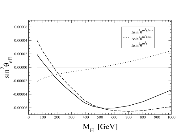
Figure 1: Two-loop electroweak contributions to the effective weak mixing angle, with a fixed W boson mass as in Tab. 2.

Table 2: Input parameters, taken from [1, 31].

input parameter	value
$M_{W}$	$80.404\pm 0.0030{\rm\;GeV}$
$M_{Z}$	$91.1876\pm 0.0021{\rm\;GeV}$
$\Gamma_{Z}$	$2.4952{\rm\;GeV}$
$m_{t}$	$172.5\pm 2.3{\rm\;GeV}$
$m_{b}$	$4.85{\rm\;GeV}$
$\Delta\alpha(M_{Z}^{2})$	$0.05907\pm 0.00036$
$\alpha_{s}(M_{Z})$	$0.119\pm 0.002$
$G_{\mu}$	$1.16637\times 10^{-5}{\rm\;GeV^{-2}}$

In order to partially cancel large perturbative effects and lower the sensitivity to input parameters, the $W$ boson mass is customarily replaced by its value determined from $\mu$ decay, or equivalently from the Fermi constant, $G_{\mu}$. The transition is made possible by the knowledge of all relevant corrections to muon decay as discussed in [17].

In view of the reparametrization, let us define the size of the complete bosonic corrections as the difference between the complete prediction of $\sin^{2}\theta^{\mbox{\footnotesize lept}}_{\mbox{\footnotesize eff}}$ and the same prediction, where pure two-loop electroweak bosonic diagrams have been omitted both in $M_{W}$ and in $\Delta\kappa$. A rough estimate of the effect can be read off Tab. 1. For example, for $M_{H}=100$ GeV and the current input parameters, where $\mbox{sin}^{2}\theta_{W}=0.2225$, the contribution to $\sin^{2}\theta^{\mbox{\footnotesize lept}}_{\mbox{\footnotesize eff}}$ from $\Delta\kappa$ is $-0.16\times 10^{-4}$, whereas using our previous results, [15, 16, 17], we find that the contribution from $M_{W}$ amounts to $0.2\times 10^{-4}$. The large cancellation in the sum gives just $0.04\times 10^{-4}$. A similar cancellation occurs for other values of $M_{H}$ over a wide range, as illustrated in Tab. 3, which also gives the complete prediction. It is important to note that, contrary to the fermionic corrections, which strongly depend on the value of the top quark mass, our result for the bosonic corrections is stable within the input parameter uncertainties and can be simply added to our fitting formula from [6], although the effect is clearly negligible.

Table 3: Higgs boson mass dependence of $M_{W}$ and $\sin^{2}\theta^{\mbox{\footnotesize lept}}_{\mbox{\footnotesize eff}}$ with $G_{\mu}$ as input parameter. Quantities with the superscript [ferm] do not contain the two-loop electroweak bosonic corrections, whereas those with the superscript [ferm+bos] do contain them. $\Delta\sin^{2}\theta_{\mbox{\footnotesize eff}}^{\mbox{}}$ is the shift induced by the bosonic corrections as described in the text. The normalization factor for $\sin^{2}\theta^{\mbox{\footnotesize lept}}_{\mbox{\footnotesize eff}}$ is $10^{-4}$, and $M_{H}$ and $M_{W}$ are given in GeV.

$M_{H}$	$M_{W}^{\mbox{[ferm]}}$	$M_{W}^{\mbox{[ferm+bos]}}$	$\sin^{2}\theta_{\mbox{\footnotesize eff}}^{\mbox{[ferm]}}$	$\sin^{2}\theta_{\mbox{\footnotesize eff}}^{\mbox{[ferm+bos]}}$	$\Delta\sin^{2}\theta_{\mbox{\footnotesize eff}}^{\mbox{}}$
100	80.3694	80.3684	0.231434	0.231438	0.04
200	80.3276	80.3270	0.231769	0.231769	0.00
600	80.2491	80.2490	0.232322	0.232327	0.05
1000	80.2134	80.2141	0.232563	0.232574	0.12

As a partial check of our calculation we have also compared the Higgs boson mass dependence of our result with the one published in [14]. Upon using the same input parameters, we have found excellent agreement as shown in Tab. 4.

Table 4: Comparison of the Higgs boson mass dependence of $\Delta\kappa$ with [14] (with $M_{W}=80.4260$ GeV and $m_{t}=178$ GeV taken from that work). The subscript “sub” denotes subtraction at $M_{H}=100$ GeV. The normalization factor is $10^{-4}$.

$M_{H}\left[GeV\right]$	$\Delta\kappa^{(\alpha^{2}),\mbox{bos}}_{\mbox{sub}}$	$\Delta\kappa^{(\alpha^{2}),\mbox{bos}}_{\mbox{sub}}$ [14]
100	0	0
200	0.266	0.265
600	0.914	0.914
1000	1.849	1.849

4 Discussion

Our calculation shows that the last piece of the two-loop electroweak corrections to the effective weak mixing angle, the one coming from purely bosonic diagrams, gives a very small contribution. In fact, being of the order of a few times $10^{-6}$, it is below the anticipated precision of the linear collider, not even to mention the current experimental accuracy. This strengthens the validity of our fitting formula [6]. Furthermore, since the recent calculation of the ${\mathcal{O}}(G_{\mu}m_{t}^{2}\alpha_{S}^{3})$ corrections to the rho parameter [12, 13], has also given a very small contribution, the results of [6] implemented in ZFITTER [32] still provide a reliable prediction for $\sin^{2}\theta^{\mbox{\footnotesize lept}}_{\mbox{\footnotesize eff}}$ under consideration of all new results.

We estimate the error from unkown higher order corrections on $\sin^{2}\theta^{\mbox{\footnotesize lept}}_{\mbox{\footnotesize eff}}$ as described in [6], including contributions for the next missing loop orders, i.e. ${\mathcal{O}}(\alpha^{3})$, ${\mathcal{O}}(\alpha^{2}\alpha_{s})$, ${\mathcal{O}}(\alpha\alpha_{s}^{3})$. We find a total theoretical error of $4.7\times 10^{-5}$, which should be taken as a very conservative error estimate, which makes it however necessary to determine further missing corrections if we want to obtain a result at the level needed by a future linear collider.

References

- [1] http://lepewwg.web.cern.ch/LEPEWWG/
- [2] R. Hawkings and K. Mönig, Eur. Phys. J. directC1, 8 (1999).
-
[3]
G. Degrassi and A. Sirlin,
Nucl. Phys. B 352, 342 (1991);
P. Gambino and A. Sirlin, Phys. Rev. D 49, 1160 (1994). - [4] A. Djouadi and C. Verzegnassi, Phys. Lett. B 195, 265 (1987); A. Djouadi, Nuovo Cim. A 100, 357 (1988); B. A. Kniehl, Nucl. Phys. B 347, 86 (1990); F. Halzen and B. A. Kniehl, Nucl. Phys. B 353, 567 (1991); B. A. Kniehl and A. Sirlin, Nucl. Phys. B 371, 141 (1992), Phys. Rev. D 47, 883 (1993); A. Djouadi and P. Gambino, Phys. Rev. D 49, 3499 (1994) [Erratum-ibid. D 53, 4111 (1996)].
- [5] K. G. Chetyrkin, J. H. Kühn and M. Steinhauser, Phys. Rev. Lett. 75, 3394 (1995), Nucl. Phys. B 482, 213 (1996).
- [6] M. Awramik, M. Czakon, A. Freitas and G. Weiglein, Phys. Rev. Lett. 93 (2004) 201805.
- [7] M. Awramik, M. Czakon, A. Freitas and G. Weiglein, Nucl. Phys. Proc. Suppl. 135, 119 (2004); A. Freitas, M. Awramik and M. Czakon, arXiv:hep-ph/0507159.
- [8] M. Awramik, M. Czakon, A. Freitas and G. Weiglein, arXiv:hep-ph/0409142.
- [9] W. Hollik, U. Meier and S. Uccirati, Nucl. Phys. B 731 (2005) 213.
- [10] M. Faisst, J. H. Kühn, T. Seidensticker and O. Veretin, Nucl. Phys. B 665, 649 (2003).
- [11] R. Boughezal, J. B. Tausk and J. J. van der Bij, Nucl. Phys. B 713 (2005) 278; R. Boughezal, J. B. Tausk and J. J. van der Bij, Nucl. Phys. B 725 (2005) 3.
- [12] Y. Schroder and M. Steinhauser, Phys. Lett. B 622 (2005) 124.
- [13] K. G. Chetyrkin, M. Faisst, J. H. Kuhn, P. Maierhoefer and C. Sturm, arXiv:hep-ph/0605201.
- [14] W. Hollik, U. Meier and S. Uccirati, Phys. Lett. B 632 (2006) 680.
- [15] A. Freitas, W. Hollik, W. Walter and G. Weiglein, Phys. Lett. B 495 (2000) 338 [Erratum-ibid. B 570 (2003) 260], Nucl. Phys. B 632 (2002) 189 [Erratum-ibid. B 666 (2003) 305]; M. Awramik and M. Czakon, Phys. Lett. B 568 (2003) 48.
- [16] M. Awramik and M. Czakon, Phys. Rev. Lett. 89 (2002) 241801; A. Onishchenko and O. Veretin, Phys. Lett. B 551 (2003) 111; M. Awramik, M. Czakon, A. Onishchenko and O. Veretin, Phys. Rev. D 68 (2003) 053004.
- [17] M. Awramik, M. Czakon, A. Freitas and G. Weiglein, Phys. Rev. D 69, 053006 (2004).
- [18] F. Jegerlehner, M. Y. Kalmykov and O. Veretin, Nucl. Phys. B 641 (2002) 285; F. Jegerlehner, M. Y. Kalmykov and O. Veretin, Nucl. Phys. B 658 (2003) 49.
- [19] V. A. Smirnov, “Applied asymptotic expansions in momenta and masses”, Berlin, Germany, Springer (2002).
- [20] M. Czakon, M. Awramik and A. Freitas, arXiv:hep-ph/0602029.
- [21] K. G. Chetyrkin and F. V. Tkachov, Nucl. Phys. B 192, 159 (1981).
- [22] S. Laporta and E. Remiddi, Phys. Lett. B 379, 283 (1996); S. Laporta, Int. J. Mod. Phys. A 15, 5087 (2000).
- [23] M. Czakon, “DiaGen/IdSolver”, unpublished; see also M. Awramik, M. Czakon, A. Freitas and G. Weiglein, Nucl. Phys. Proc. Suppl. 135 (2004) 119.
- [24] A. V. Kotikov, Phys. Lett. B 254, 158 (1991); A. V. Kotikov, Phys. Lett. B 259, 314 (1991).
- [25] E. Remiddi, Nuovo Cim. A 110, 1435 (1997).
- [26] M. Czakon, arXiv:hep-ph/0511200.
- [27] V. A. Smirnov, Phys. Lett. B 460, 397 (1999).
- [28] J. B. Tausk, Phys. Lett. B 469, 225 (1999).
- [29] C. Anastasiou and A. Daleo, arXiv:hep-ph/0511176.
- [30] T. Binoth and G. Heinrich, Nucl. Phys. B 585, 741 (2000); T. Binoth and G. Heinrich, Nucl. Phys. B 680, 375 (2004).
- [31] S. Eidelman et al. [Particle Data Group Collaboration], Phys. Lett. B 592 (2004) 1, also 2005 partial update for edition 2006, available on http://pdg.lbl.gov
- [32] A.B. Arbuzov, M. Awramik, M. Czakon, A. Freitas, M.W. Grünewald, K. Mönig, S. Riemann, T. Riemann, Comput. Phys. Commun. 174: 728-758, 2006.