FCNC Top Quark Decays in Extra Dimensions

Abstract

The flavor changing neutral top quark decay $t\rightarrow cX$ is computed, where $X$ is a neutral standard model particle, in a extended model with a single extra dimension. The cases for the photon, $X=\gamma$, and a Standard Model Higgs boson, $X=H$, are analyzed in detail in a non-linear $R_{\xi}$ gauge. We find that the branching ratios can be enhanced by the dynamics originated in the extra dimension. In the limit where $1/R>>m_{t}$, we have found $Br(t\to c\gamma)\simeq 10^{-10}$ for $1/R=0.5\,TeV$. For the decay $t\to cH$, we have found $Br(t\to cH)\simeq 10^{-10}$ for a low Higgs mass value. The branching ratios go to zero when $1/R\to\infty$.

I Introduction

Flavor changing neutral currents (FCNC) are very suppressed in the standard model (SM): there are no tree level contributions and at one loop level the charged currents operate with the Glashow-Iliopoulos-Maiani (GIM) mechanism. The branching ratio for top quark FCNC decays into charm quarks are of the order of $10^{-11}$ for $t\rightarrow cg$ and $10^{-13}$ for $t\rightarrow c\gamma,(Z)$ in the framework of the SM sm1 ; sm2 . This suppression can be traced back to the loop amplitudes: they are controlled by down-type quarks, mainly by the bottom quark, resulting in a $m_{b}^{4}/M_{W}^{4}$ factor which can be compared to the enhancement factor that appears in the $b\rightarrow s\gamma$ process where the top quark mass $m_{t}$ is involved instead of $m_{b}$ in this factor. This fourth power mass ratio is generated by the GIM mechanism and is responsible for the suppression beyond naive expectations based on dimensional analysis, power counting and Cabibbo-Kobayashi-Maskawa (CKM)-matrix elements involved. The top quark decay into the SM Higgs boson is even more suppressed sm1 ; sm2 : $Br(t\rightarrow cH)\sim 10^{-13}-10^{-15}$ for $M_{Z}\leq M_{H}\leq 2M_{W}$. These rates are far below the reach of any foreseen high luminosity collider in the future. The highest FCNC top quark rate in the SM is $t\rightarrow cg$, but this value is still six orders of magnitude below the possibility of observation at the LHC.

The discovery of these FCNC effects would be a hint of new physics because of the large suppression in the SM. These FCNC decay modes can be strongly enhanced in scenarios beyond the SM, where some of them could be even observed at the LHC or ILC. New physics effects in extended Higgs sector models, SUSY and left-right symmetric models were studied in references [1-5]. For example, in various SUSY scenarios the branching ratios can go up to the value $10^{-5}$ for the decay $t\rightarrow cg$. Also, virtual effects of a $Z^{\prime}$ gauge boson on these rare top quark decays were studied. The decay $t\rightarrow c\gamma$ has been analyzed in reference z1 , it has been shown that $B(t\rightarrow c\gamma)$ is at the $10^{-6}$ level in topcolor assisted technicolor models for $m_{Z}^{\prime}=1\,TeV$, which would allow the detection of this process at future colliders.

On the other hand, the use of effective Lagrangians in parameterizing physics beyond the SM has been studied extensively in FCNC top quark couplings and decays el1 ; el2 ; el3 . This formalism generates a model-independent parameterization of any new physics characterized by higher dimension operators. Under this approach, several FCNC transitions have been also significantly constrained: $t\to c\gamma$ tosc ; tcg , $t\to cg$ tcg ; cord , $l_{i}\to l_{j}\gamma$ lar and $H\to l_{i}l_{j}$ dia .

New physics effects have also been introduced in models with large extra dimensions (ED) ed . In recent years, these models have been a major source of inspiration for beyond the SM physics in the ongoing research. In these scenarios the four dimensional SM emerges as the low energy effective theory of models living in more than four dimensions, where these extra dimensions are orbifolded. The presence of infinite towers of Kaluza-Klein (KK) modes are the remanent of the extended dimensional dynamics at low energies. The size of the extra dimensions can be unexpectedly large, with $1/R$ at the scale of a few $TeV$ without contradicting the present experimental data eds . Then, if these KK-modes are light enough, they could be produced in the near future at the next generation of colliders. Scenarios where all the SM fields, fermions as well as bosons, propagate in the bulk are known as ”universal extra dimensions”ued ; pom . In these theories the number of KK-modes is conserved at each elementary vertex and the coupling of any excited KK-mode to two zero modes is prohibited. Then the constraints on the size of the extra dimensions obtained from the SM precision measurements are less stringent than in the case where there is no conservation of the KK particles (non universal extra dimensions).

The impact of the new physics coming from UED models has been widely studied and constraints on the parameter $1/R$ have been obtained. Analysis of the precision electroweak observables led to the lower bound $1/R\gtrsim 700-800$ GeV for a light Higgs boson mass and to $1/R\gtrsim 300-400$ GeV for a heavy Higgs boson mass russell . On the other hand, using the process $b\to s\gamma$, the resulting bound on the inverse compactification radius is $1/R\gtrsim 250$ GeV bsg . Moreover, a recent analysis making use of the exclusive branching ratio $B\to K^{*}\gamma$ shows that under conservative assumptions $1/R\gtrsim 250$ GeV bkg . And from the inclusive radiative $\bar{B}\to X_{s}\gamma$ decay, a lower bound on $1/R\gtrsim 600$ GeV at $95\%$ C.L. can be obtained and it is independent of the Higgs boson mass value bxs . Contributions from UED models have been considered on several FCNC processes, reference burasydemas has found that the processes $K_{L}\to\pi^{0}e^{+}e^{-},\Delta M_{s},K^{+}\to\pi^{+}\nu\bar{\nu},K_{L}\to\pi^{0}\nu\bar{\nu},B_{d,s}\to X_{d,s}\nu\bar{\nu},K_{L}\to\mu^{+}\mu^{-},B_{d,s}\to\mu^{+}\mu^{-},B\to X_{s}\mu^{+}\mu^{-}$ for $1/R\approx 300$ GeV are enhanced relative to the SM expectation and the processes $B\to X_{s}\gamma,B\to X_{s}g,\epsilon^{\prime}/\epsilon$ are suppressed respect to the SM. In general, the present data on FCNC processes are consistent with $1/R\gtrsim 300$ GeV burasydemas ; report . Exclusive $B\to K^{*}l^{+}l^{-},B\to K^{*}\nu\bar{\nu}$ and $B_{s}$ decays bkg ; raros1 have been studied in the framework of the UED scenario and also rare semileptonic $\Lambda_{b}$ decays raros2 .

In this paper we study the FCNC decays of the top quark in a universal extra dimension theory where all the SM fields live in five dimensions. In particular, we compute the $t\rightarrow c\gamma$ and $t\rightarrow cH$ decay modes in a non linear $R_{\xi}$. This gauge has the advantage of a reduced number of Feynman diagrams as well as simplified Ward identities. These facts facilitates and clarify the calculation.

The paper is organized as follows: in section II we present the general framework for the five dimensional Lagrangian and derive the corresponding four dimensional Lagrangian and Feynman rules. In section III and IV we compute the decays mode $t\rightarrow c\gamma$ and $t\rightarrow cH$ respectively, and discuss the hypothesis implicit in the calculation. Finally, in section V we present some conclusions. In the Appendix (section VI) we show the terms in the Lagrangian that are important for the Feynman rules in our calculation.

II The Model

We begin presenting the SM Lagrangian in five dimensions; let $x=0,1,2,3$ be the normal coordinates and $x^{4}=y$ the fifth one. The fifth extra dimension is compactified on the orbifold $S^{1}/Z_{2}$ orbifold of size $R$ which is the compatification radius. We consider a generalization of the SM where the fermions, the gauge bosons and the Higgs doublet propagate in the five dimensions. The Lagrangian $L$ can be written as

$$L=\int d^{4}x\,dy\,({\cal L}_{A}+{\cal L}_{H}+{\cal L}_{F}+{\cal L}_{Y})$$ (1)

with

$${\cal L}_{A} = -\frac{1}{4}W^{MNa}W^{a}_{MN}-\frac{1}{4}B^{MN}B_{MN},$$

$${\cal L}_{H} = (D_{M}\Phi)^{\dagger}D^{M}\Phi-V(\Phi),$$

$${\cal L}_{F} = \,\left[\,\overline{Q}(i\Gamma^{M}D_{M})Q+\overline{U}(i\Gamma^{M}D_{M})U+\overline{D}(i\Gamma^{M}D_{M})D\right],$$

$${\cal L}_{Y} = -\overline{Q}\widetilde{Y}_{u}\Phi^{c}U-\,\overline{Q}\widetilde{Y}_{d}\Phi D+h.c.$$ (2)

The numbers $M,N=0,1,2,3,5$ denote the five dimensional Lorentz indexes, $W^{a}_{MN}=\partial_{M}W^{a}_{N}-\partial_{N}W^{a}_{M}+\widetilde{g}\epsilon^{abc}W^{b}_{M}W^{c}_{N}$ is the strength field tensor for the $SU(2)_{L}$ electroweak gauge group and $B_{MN}=\partial_{M}B_{N}-\partial_{N}B_{M}$ is that of the $U(1)_{Y}$ group. The gauge fields depend on $x$ and $y$. The covariant derivative is defined as $D_{M}\equiv\partial_{M}-i\widetilde{g}\,W^{a}_{M}T^{a}-i\widetilde{g}\,^{\prime}B_{M}Y$, where $\widetilde{g}$ and $\widetilde{g}\,^{\prime}$ are the five dimensional gauge couplings constants for the groups $SU(2)_{L}$ and $U(1)_{Y}$ respectively, and $T^{a}$ and $Y$ are the corresponding generators. The five dimensional gamma matrices $\Gamma_{M}$ are $\Gamma_{\mu}=\gamma_{\mu}$ and $\Gamma_{4}=i\gamma_{5}$ with the metric tensor given by $g_{MN}=(+,-,-,-,-)$. The matter fields $Q$, $D$ and $U$ are fermionic four components spinors with the same quantum numbers as the corresponding SM fields. To simplify the notation we have suppressed the $SU(2)$ and color indices. The standard and charge conjugate doublet standard Higgs fields are denoted by $\Phi(x,y)$ and $\Phi^{c}(x,y)=i\tau^{2}\Phi^{*}(x,y)$; $\widetilde{Y}_{u,d}$ are the Yukawa matrices in the five dimensional theory responsible for the mixing of different families whose indices were suppressed in the notation for simplicity. We have not included in Eq. (2) the leptonic sector nor the $SU(3)_{c}$ dynamics because it is not relevant for our proposes. The low energy theory will only have zero modes for fields that are even under $Z_{2}$ symmetry: this is the case for the Higgs doublet that we choose to be even under this symmetry in order to have a standard zero mode Higgs field. The Fourier expansions of the fields are given by:

$$B_{\mu}(x,y) = \frac{1}{\sqrt{\pi R}}B_{\mu}^{(0)}(x)+\frac{\sqrt{2}}{\pi R}\sum_{n=1}^{\infty}B_{\mu}^{(n)}(x)\cos\left(\frac{ny}{R}\right),$$

$$B_{5}(x,y) = \frac{\sqrt{2}}{\pi R}\sum_{n=1}^{\infty}B_{5}^{(n)}(x)\sin\left(\frac{ny}{R}\right),$$

$$Q(x,y) = \frac{1}{\sqrt{\pi R}}Q_{L}^{(0)}(x)+\frac{\sqrt{2}}{\pi R}\sum_{n=1}^{\infty}\left[Q_{L}^{(n)}(x)\cos\left(\frac{ny}{R}\right)+Q_{R}^{(n)}\sin\left(\frac{ny}{R}\right)\right],$$

$$U(x,y) = \frac{1}{\sqrt{\pi R}}U_{R}^{(0)}(x)+\frac{\sqrt{2}}{\pi R}\sum_{n=1}^{\infty}\left[U_{R}^{(n)}(x)\cos\ \left(\frac{ny}{R}\right)+U_{L}^{(n)}\sin\left(\frac{ny}{R}\right)\right],$$

$$D(x,y) = \frac{1}{\sqrt{\pi R}}D_{R}^{(0)}(x)+\frac{\sqrt{2}}{\pi R}\sum_{n=1}^{\infty}\left[D_{R}^{(n)}(x)\cos\ \left(\frac{ny}{R}\right)+D_{L}^{(n)}\sin\left(\frac{ny}{R}\right)\right].$$ (3)

The expansions for $B_{\mu}$ and $B_{5}$ are similar to the expansions for the gauge fields and the Higgs doublet (but this last one without the $\mu$ or $5$ Lorentz index). It is by integrating the fifth $y$ component in Eq. (1) that we obtain the usual interaction terms and the KK spectrum for ED models.

The interaction terms relevant for our calculation will be written in a non-linear $R_{\xi}$ gauge (see for details des and the first reference in esm3 ). For example, in this gauge there is no mixing between the gauge bosons and the charged and neutral unphysical Higgs fields. Besides, the interaction terms are simplified in such a way that there are no trilinear terms such as $W_{\mu}^{+}G_{W}^{-}A_{\mu}$, where $G_{W}^{-}$ is an unphysical Higgs field. We are interested in the third family of quarks and $Q_{t}^{(n)}$ and $Q_{b}^{(n)}$ are the upper and lower parts of the doublet $Q$. Similarly, the $U_{t}^{(n)}$ and $D_{b}^{(n)}$ are the KK modes of the usual right-handed singlet top and bottom quarks, respectively. There is a mixing between the mass and gauge eigenstates of the KK top quarks ($Q_{t}^{(n)}$ and $U_{t}^{(n)}$) where the mixing angle is given by $\tan(2\alpha_{t}^{n})=m_{t}/m_{n}$ with $m_{n}=n/R$. For the $b$ quark the mixing is quite similar, but at leading order the only masses that remain are $m_{t}$ and $m_{n}$ and in this limit the mixing angle is zero. This leads to the spectrum $m_{Q_{b}^{n}}=m_{n}$ and $m_{Q_{t}^{n}}=m_{U^{n}}=\sqrt{m_{t}^{2}+m_{n}^{2}}$ for the excited modes of the third family. After dimensional reduction, the fifth components of the charged gauge fields, $W_{5}^{-(n)}$, mix with the KK modes of the charged component $\phi^{-(n)}$ of the Higgs doublet. The unmixed states are thus the charged physical boson $G_{W}^{-(n)}$ excited state and a would be Goldstone boson $\phi_{G}^{-(n)}$ that contribute to the mass of the KK gauge bosons:

$$\phi_{G}^{\pm(n)} = \frac{m_{n}W_{5}^{\pm(n)}+iM_{W}\phi^{\pm(n)}}{\sqrt{m_{n}^{2}+M_{W}^{2}}}\stackrel{{\scriptstyle\stackrel{{\scriptstyle n\not=0}}{{M_{W}\to 0}}}}{{\longrightarrow}}W_{5}^{\pm(n)}~{},$$

$$G_{W}^{\pm(n)} = \frac{iM_{W}W_{5}^{\pm(n)}+m_{n}\phi^{\pm(n)}}{\sqrt{m_{n}^{2}+M_{W}^{2}}}\stackrel{{\scriptstyle\stackrel{{\scriptstyle n\not=0}}{{M_{W}\to 0}}}}{{\longrightarrow}}\phi^{\pm(n)}~{}.$$ (4)

The final expression for the lagrangian can be found in the Appendix A, where we show the terms that contribute to the decays we are interested in.

III The $t\rightarrow c\,\gamma$ decay rate

In this section, we present the calculation at one-loop level of the $t\to c\gamma$ process in the framework of a 5-dimensional universal ED model. We start with a naive calculation comparing the decay widths calculate in the SM and ED model and assuming that in the ED model only the third generation is running in the loop. The one loop SM width for the top quark decay into a charm quark plus a gauge boson can be approximated by

$$\Gamma(t\to cV)\simeq|V_{bc}|^{2}\,\alpha\,\alpha_{em}^{2}\,m_{t}\,\left(\frac{m_{b}}{M_{W}}\right)^{4}\,\left(1-\frac{m_{V}^{2}}{m_{t}^{2}}\right)^{2}$$ (5)

where for a photon, the neutral gauge boson and a gluon we have $\alpha=\alpha_{em}$ ($V=\gamma,Z$) or $\alpha=\alpha_{s}$ ($V=g$) respectively. These results can be compared to the ones expected for extra dimensions, where the ratio $m_{b}/M_{W}$ is replaced by $M_{W}/m_{n}$. Using these approximations we can naively estimate the ratio,

$$\frac{\Gamma(t\to c\gamma)_{ED}}{\Gamma(t\to c\gamma)_{SM}}\simeq\left[\frac{\left(\sum_{n}(M_{W}/m_{n})^{2}\right)^{2}}{\left(m_{b}/M_{W}\right)^{4}}\right].$$ (6)

The sum on the KK tower of excited states can be evaluated as we will explain later in the text and we obtain

$$\frac{\Gamma(t\to c\gamma)_{ED}}{\Gamma(t\to c\gamma)_{SM}}=\frac{\pi^{4}}{36}\,\left[\frac{\left(M_{W}/(1/R)\right)}{(m_{b}/M_{W})}\right]^{4}\simeq 1.2\times 10^{2}$$ (7)

for $R^{-1}\sim 0.5\,TeV$. We have already mentioned that the SM prediction for the branching fraction for the decay $t\to c\gamma$ is of the order $Br(t\to c\gamma)\sim 10^{-12}$. Then, from Eq. (7) the branching fraction for ED models is $Br(t\to c\gamma)_{ED}\sim 1\times 10^{-10}$ for $R^{-1}=0.5$ TeV.

The naive result on the $\Gamma(t\to c\gamma)_{ED}$ motivates a complete analysis of the one loop amplitude in extra dimensions. The general transition $q_{i}\rightarrow q_{j}+\gamma$ for arbitrary quark flavors $i,j$ in a non linear $R_{\xi}$ gauge was studied in reference des , where it was found that a reduced number of Feynman diagrams as well as simplified Ward identities greatly facilitates the calculation in this $R_{\xi}$ gauge.

For on-shell quarks and real photons the transition matrix element is given by

$$M_{\mu}=i\sigma_{\mu\nu}k^{\nu}(F_{2}^{L}m_{c}P_{L}+F_{2}^{R}m_{t}P_{R}),$$ (8)

where $k_{\mu}$ is the photon momentum, $P_{R,L}=(1\pm\gamma_{5})/2$ and the magnetic transition form factors $F_{2}^{L,R}$ are

$$2F_{2}^{L}\,m_{c}=(B_{1}+B_{3}+2B_{5})m_{t}-A_{3}m_{c}+A_{12}-2A_{11},$$ (9)

$$2F_{2}^{R}\,m_{t}=(A_{1}+A_{3}+2A_{5})m_{t}-B_{3}m_{c}+B_{12}-2B_{11},$$ (10)

where the $A_{i},B_{i}$ form factors are gotten from the most general Lorentz structure of the renormalized proper vertex des .

Electromagnetic gauge invariance restricts the amplitude of this decay to the form

$${\cal M}(t\to c\gamma)=\frac{ieg^{2}}{2^{6}c^{2}_{W}\pi^{2}m_{t}^{2}}\,\epsilon_{\alpha}^{*}\,k_{\mu}\,(2\widetilde{F}_{2}^{R}m_{t})\,\bar{u}_{c}\sigma^{\alpha\mu}P_{R}u_{t}$$ (11)

where $c_{W}$ is the cosine of the weak mixing angle and the form factors $F_{2}^{R}$ and $\widetilde{F}_{2}^{R}$ are related by

$$F_{2}^{R}m_{t}=\frac{eg^{2}}{32c_{W}^{2}\pi^{2}\,m_{t}}\widetilde{F}_{2}^{R}.$$ (12)

The decay width for this process can be written as

$$\Gamma(t\rightarrow c\,\gamma)=\frac{\alpha^{3}m_{t}}{2^{9}\pi^{2}s_{w}^{4}c_{w}^{4}}|\widetilde{F}_{2}^{R}|^{2}\approx 4.8\times 10^{-7}|\widetilde{F}_{2}^{R}|^{2}.$$ (13)

In order to perform the one loop calculation, we consider two scenarios. The first one, when the mass of the excited states associated to the quarks from the three low-energy families are quasi-degenerated at tree level, without any kind of radiative corrections to KK masses. In this case, when the excitations coming from the other quarks are taken into account, the transition amplitude for the process $t\to c\gamma$ takes the form

$$\propto \sum_{i=d,s,b}V_{ti}V_{ci}^{*}\frac{1}{(n/R)^{2}+m_{i}^{2}}$$ (14)

$$\approx V_{tb}V_{cb}^{*}\frac{1}{(n/R)^{2}}\frac{m_{b}^{2}}{(n/R)^{2}}$$

where the last line can be obtained using the unitarity of the CKM matrix and considering that the electroweak corrections of the first two families are of order zero. $m_{i}$ is the mass of the down quark running into the loop. Therefore in this scenario, we notice that the naive expectation of the decay width $\Gamma(t\to c\gamma)$ given by (7) is suppressed by the factor $(m_{b}/(n/R))^{4}$, and then the final result, including the KK states, is smaller than the SM value.

In the second scenario, we consider that the most important contribution to the loop correction comes from the excited KK states associated to the third generation. This is a more realistic scenario because there is a mass hierarchy in the KK states from the different families, such as at low energy. We should mention that in universal extra dimension theories, the fixed points from the orbifold break the translational symmetry of the extra dimension and it is possible to introduce new interactions on the branes. In these new interactions, there are counterterms that cancel the divergences of the radiative corrections, mass terms, and mixing terms from the different family KK modes fixpoint . All our results are presented in the context of this scenario.

Some of the Feynman rules for the model of Section II can be found in the Appendix where all the relevant terms are shown. In Figure 1, we illustrate the topology of the one-loop diagrams that are contributing.

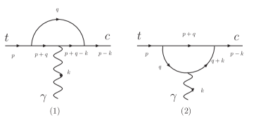
Figure 1: Diagrams contributing to the $t\rightarrow c\,\gamma$ decay in the non linear $R_{\xi}$ gauge.

In all the decays we are interested in, we neglect corrections of order $(m_{c}/M_{W})^{2}$. The mixing angle between the gauge and mass eigenstates for the KK excitations of the quarks are written in section II and are zero for the leading order approximation. Other possible contributions are neglected due to the Yukawa coupling constants. For example, diagrams involving $G_{W}^{-(n)}\bar{Q}_{b}^{(n)}c_{R}^{(0)}$ are proportional to the Yukawa coupling $\lambda_{c}$, and therefore to $m_{c}^{2}$. Diagrams with $G_{W}^{-(n)}\,\bar{D}_{b}^{(n)}\,t_{L}^{(0)}$ in the loop are proportional to $\lambda_{b}^{2}$ and then to $m_{b}^{2}$ and can be neglected.

The leading contributions of type 1 diagrams (see figure 1) to the decay come from the following particles circulating in the loop:

$$W_{5}^{(n)}Q_{b}^{(n)}Q_{b}^{(n)},\;\;\;W_{\mu}^{(n)}Q_{b}^{(n)}Q_{b}^{(n)},\;\;\;G_{W}^{(n)}Q_{b}^{(n)}Q_{b}^{(n)},\;\;\;G_{W}^{(n)}D_{b}^{(n)}D_{b}^{(n)}.$$ (15)

where the external photon is coupled to the fermion in the loop. The sum of all these diagrams gives, for the form factor $F_{2}^{R}$, the following expression

$$2F_{2}^{R} = \frac{2}{3}g^{2}e\,V_{tb}V_{cb}^{*}\,\frac{i}{16\pi^{2}}\,\int_{0}^{1}\,dz\int_{0}^{1-z}\,dw\frac{1-w-z}{\widetilde{X}}$$ (16)

$$\times\left[z+(1-w)+z\frac{m_{b}^{2}}{M_{W}^{2}}\right],$$

where the factor $\widetilde{X}$ comes from the dimensional regularization tricks of the product of inverse propagators of the particles circulating in the loop

$$\widetilde{X}=m^{2}_{t}z^{2}+m_{t}^{2}wz-m_{t}^{2}z+m_{n}^{2}.$$ (17)

The main contribution of type 2 diagrams (see figure 1) is the one with KK excitation of the standard model gauge boson or a scalar field circulating in the loop which are coupled to the external photon:

$$W_{\mu}^{(n)}W_{\mu}^{(n)}Q_{b}^{(n)},\;\;\;W_{5}^{(n)}W_{5}^{(n)}Q_{b}^{(n)},\;\;\;G_{W}^{(n)}G_{W}^{(n)}D_{b}^{(n)},\;\;\;G_{W}^{(n)}G_{W}^{(n)}Q_{b}^{(n)},$$

$$(G_{W}^{(n)}W_{\mu}^{(n)}Q_{b}^{(n)}+W_{\mu}^{(n)}G_{W}^{(n)}Q_{b}^{(n)}).$$ (18)

These terms contribute to the $F_{2}^{R}$ form factor with the following expression

$$2F_{2}^{R} = -g^{2}e\frac{i}{16\pi^{2}}\,V_{tb}V_{cb}^{*}\,\int_{0}^{1}\,dz\int_{0}^{1-z}\,dw\frac{1}{\widetilde{X}}\left\{4(2-3w-4z+2wz+2z^{2})\right.$$ (19)

$$- (1-w-z)\left.\left[(w+z)-(w+z-1/2)\frac{m_{b}^{2}}{M_{W}^{2}}\right]\right\}.$$

For a mass scale of the excited states much higher than the electroweak scale, i.e., $m_{n}\gg m_{t}$, the denominator can be approximated by $\widetilde{X}\simeq m_{n}^{2}$. We also consider that the excited quarks rotate from interaction to mass eigenstates with the same matrix of the ordinary quarks. So, in the Yukawa lagrangian the interactions $\bar{Q}_{bL}t_{R}^{(0)}G_{W}^{-(n)}$ and $\bar{Q}_{bL}c_{R}^{(0)}G_{W}^{-(n)}$ are proportional to $V_{tb}$ and $V_{cb}$ respectively, in the mass eigenstates. If we compare the leading contribution coming from these diagrams respect to the SM contribution sm2 , it is

$$\frac{1}{m_{n}^{2}}\,:\,\frac{m_{b}^{2}}{M_{W}^{2}}\frac{1}{M_{W}^{2}}.$$ (20)

The numerical estimation of all these contributions is straightforward. All the excited mass terms are proportional to $n/R$, except for the electroweak correction coming from the symmetry breaking. From the numerical point of view this correction does not change the results and can be neglected without modifying the final estimates. Based on these hypothesis, we can also take $\widetilde{X}\simeq m_{n}^{2}$ and, then, the sum over all the KK excited states can be easily done, as

$$\sum_{n}\frac{1}{\widetilde{X}}\simeq\sum_{n}\frac{1}{\left(\frac{n}{R}\right)^{2}}=\frac{\pi^{2}}{6}\frac{1}{\left(\frac{1}{R}\right)^{2}}$$ (21)

where in any numerical estimate $1/R\simeq{\cal{O}}(1)$ TeV.

Thus, within this approximation, the sum over all the excited KK states is equivalent to multiply the results obtained for the first KK excited state by the factor $\pi^{2}/6$. The sum of all contributions using equations (16) and (19) gives,

$$2F_{2}^{R} = \frac{g^{2}e}{3}V_{tb}V_{cb}^{*}\frac{i}{16\pi^{2}}\int_{0}^{1}\,dz\int_{0}^{1-z}\,dw\frac{1}{\widetilde{X}}\left\{-22+35w-w^{2}\right.$$ (22)

$$+ \left.51z-30wz-29z^{2}+(-4z^{2}-4wz+10z+6w+3)\frac{m_{b}^{2}}{2M_{W}^{2}}\right\}$$

$$\approx \frac{g^{2}e}{18m_{n}^{2}}V_{tb}V_{cb}^{*}\frac{i}{16\pi^{2}}\left\{-\frac{5}{2}+11\frac{m_{b}^{2}}{M_{W}^{2}}\right\}.$$

By using equations (13) and (12), the numerical value for the decay width is

$$\Gamma(t\rightarrow c\gamma)=1.65\times 10^{-10}\,GeV\;\;,$$ (23)

for $R^{-1}=0.5$ TeV, and the branching fraction is

$$Br(t\rightarrow c\gamma)\equiv\frac{\Gamma(t\rightarrow c\gamma)}{\Gamma(t\rightarrow Wb)}=1.08\times 10^{-10}.$$ (24)

This result shows a branching ratio above the SM one, two orders of magnitude.

IV The $t\rightarrow c\,H$ decay rate

The invariant amplitude for the flavor changing decay of a top quark into a charm quark plus a SM Higgs particle can be written as

$${\cal M}(t\to cH)=\overline{u}_{c}(p)\,\left(F_{L}P_{L}+F_{R}P_{R}\right)\,u_{t}(k),$$ (25)

where $F_{L}$ and $F_{R}$ are form factors. In our notation we identify the external scalar Higgs $H$ with the zero mode Higgs field $h^{(0)}$. From this amplitude we can compute the decay width

$$\Gamma(t\to cH)\,=\,\frac{m_{t}}{32\pi}\,\left(1-\frac{m_{H}^{2}}{m_{t}^{2}}\right)^{2}\,\left(|F_{L}|^{2}+|F_{R}|^{2}\right).$$ (26)

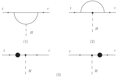
Figure 2: Feynman diagrams for the $t\rightarrow c\,H$ decay in extra dimensions.

The leading diagrams that contribute to the decay are shown in Figure 2. The leading group of type 1 diagrams in figure 2 is the one with KK excitations of the SM quarks circulating in the loop which are coupled to the external higgs:

$$W_{\mu}^{(n)}Q_{b}^{(n)}D_{b}^{(n)},\;\;\;G_{W}^{(n)}Q_{b}^{(n)}Q_{b}^{(n)},\;\;\;W_{5}^{(n)}Q_{b}^{(n)}D_{b}^{(n)}.$$ (27)

In this case, the external Higgs is coupled to the excited quark $Q_{b}$ generating a flavor changing $\bar{Q}^{(n)}D_{b}h^{(0)}$ (see the appendix), which is proportional to the bottom quark mass $m_{b}$. The contributions to the $F_{L}$, $F_{R}$ form factors are of the order of zero at leading order, ${\it i.e.}\,F_{L}=F_{R}\approx 0$.

The leading diagrams of type 2 in figure 2 is the one with KK excitations of the standard model gauge bosons and scalar fields circulating in the loop which are coupled to the external higgs boson $h^{(0)}$:

$$W_{5}^{(n)}W_{5}^{(n)}Q_{b}^{(n)},\;\;\;G_{W}^{(n)}G_{W}^{(n)}Q_{b}^{(n)},\;\;\;W_{\mu}^{(n)}W_{\mu}^{(n)}Q_{b}^{(n)},\;\;\;W_{\mu}^{(n)}G_{W}^{(n)}Q_{b}^{(n)},$$

$$G_{W}^{(n)}W_{\mu}^{(n)}Q_{b}^{(n)},\;\;\;(W_{5}^{(n)}G_{W}^{(n)}Q_{b}^{(n)}+G_{W}^{(n)}W_{5}^{(n)}Q_{b}^{(n)})\,,$$ (28)

and these contribute to the form factor with the following expressions:

$$F_{L} = \,g^{3}V_{tb}V_{cb}^{*}\frac{i}{16\pi^{2}}\,\int_{0}^{1}\,dz\int_{0}^{1-z}\,dw\frac{1}{\widetilde{X}}\left\{2(1-w)m_{t}M_{W}\right.$$

$$- \left.\left[(z-1)(w+z)m_{t}^{2}+w(z-2)m_{h}^{2}\right]\frac{m_{t}}{m_{W}}\right\}$$

$$F_{R} = g^{3}V_{tb}V_{cb}^{*}\frac{i}{16\pi^{2}}\,\int_{0}^{1}\,dz\int_{0}^{1-z}\,dw\frac{1}{\widetilde{X}}\left\{wm_{t}M_{W}\right\}.$$ (29)

After evaluating the parametric integrals, the form factors are given by

$$F_{L} = \frac{g^{3}}{6m_{n}^{2}}\,V_{tb}V_{cb}^{*}\,\frac{i}{16\pi^{2}}\left\{8M_{W}m_{t}+\frac{5m_{t}^{3}}{M_{W}}+\frac{7m_{h}^{2}m_{t}}{2m_{W}}\right\},$$

$$F_{R} = \frac{g^{3}}{6m_{n}^{2}}\,V_{tb}V_{cb}^{*}\,\frac{i}{16\pi^{2}}\left\{M_{W}m_{t}\right\}.$$ (30)

Finally, the type 3 diagrams in figure 2 coming from a renormalized flavor changing fermion line, do not contribute at leading order to the decay width. The first one of these diagrams is proportional to the charm quark mass because of the Higgs coupling, and therefore is negligible. For a similar reason, the second diagram has a top quark mass factor, but the self-energy part introduces the charm quark mass and this contribution is suppressed respect to the leading order.

From these form factors and equation (26), we compute the $t\to cH$ decay width. Finally, the branching ratio is $Br(t\to cH)=1.08\times 10^{-10}$, for $m_{H}=120$  GeV .

V Conclusions

We have computed the decay widths $\Gamma(t\to c\,\gamma)$ and $\Gamma(t\to c\,H)$ in a universal extra dimension model with a single extra dimension, where we have considered that the most important contribution to the loop correction comes from the excited KK states associated to the third generation. The results show a branching ratio that is above the SM one. The branching ratios for these two decay widths are of the order of $10^{-10}$.

There is a strong dependence on top quark mass $m_{t}$ in the amplitude of the $t\to cH$ process, it is coming from the type 2 diagrams in figure 2 with an excited scalar in the loop, resulting in a $m_{t}^{3}/M_{W}^{3}$ factor. When we take the limit $m_{n}\gg m_{t}$, we find that the decay widths for the $t\to c\gamma,(H)$ processes are decoupled respect to the new scale $1/R$ and they go to zero. Considering that the excited states of the quarks are quasi-degenerated and the unitarity of the CKM matrix, the amplitudes for the flavor changing decay $t-c$ due to the contribution of the excited states of the quarks, are suppressed by the factor $(m_{b}/(n/R))^{2}$, and the predicted values are smaller than the SM predictions.

VI acknowledgements

R. Martinez acknowledge the financial support from Fundaci n Banco de la Republica.

VII Appendix

The Lagrangian can be separated in different terms as in the following sum:

$$L=\sum_{m=1,2,3}\sum_{n=1}^{\infty}L_{m}^{(n)}.$$ (31)

After symmetry breaking the interaction terms are included in the terms $L_{1}^{(n)}$ up to $L_{3}^{(n)}$. The first one, $L_{1}^{(n)}$ is

$$L_{1}^{(n)}=\frac{gm_{t}}{\sqrt{2}M_{W}}\bar{Q}_{bL}^{(n)}t_{R}^{(0)}G_{W}^{-(n)}-\frac{gm_{b}}{\sqrt{2}M_{W}}\bar{D}_{bR}^{(n)}t_{L}^{(0)}G_{W}^{-(n)}+h.c.$$ (32)

The second term, $L_{2}^{(n)}$ has the excited gauge boson-fermion interactions:

$$L_{2}^{(n)} = \frac{2}{3}\,e\,A_{\mu}^{(0)}\left[\bar{Q}_{t}^{(n)}\gamma^{\mu}{Q}_{t}^{(n)}+\bar{u}_{t}^{(n)}\gamma_{\mu}\bar{u}_{t}^{(n)}\right]+\left\{\frac{g}{\sqrt{2}}W_{\mu}^{+(n)}\bar{Q}_{bL}^{(n)}\gamma^{\mu}t_{L}^{(0)}\right.$$ (33)

$$+ \left.i\,e\,A_{\mu}^{(0)}\left[G_{W}^{-(n)}\partial^{\mu}G_{W}^{+(n)}+W_{5}^{-(n)}\partial^{\mu}W_{5}^{+(n)}\right]+\frac{g}{\sqrt{2}}\bar{Q}_{bR}^{(n)}t_{L}^{(0)}W_{5}^{-(n)}\right.$$

$$+ \left.2\,e\,\frac{n}{R}A_{\mu}^{(0)}\left[W^{-(n)}_{\mu}W_{5}^{+(n)}-W^{+(n)}_{\mu}W_{5}^{-(n)}\right]+h.c.\right\}$$

And the third term has the neutral Higgs boson interactions:

$$L_{3}^{(n)} = -\frac{gm_{t}}{2M_{W}}\bar{Q}_{t}^{(n)}U_{t}^{(n)}h^{(0)}-\frac{gm_{b}}{2M_{W}}\bar{Q}_{b}^{(n)}D_{b}^{(n)}h^{(0)}$$ (34)

$$+ gM_{W}W_{5}^{+(n)}W_{5}^{-(n)}h^{(0)}+gM_{W}W_{\mu}^{+(n)}W_{\mu}^{-(n)}h^{(0)}$$

$$- \frac{gm_{h}^{2}}{2M_{W}}G_{W}^{+(n)}G_{W}^{-(n)}h^{(0)}$$

$$+ \left\{i\frac{g}{2}\frac{n}{R}W_{5}^{(n)}G_{W}^{+(n)}h^{(0)}+i\frac{g}{2}W_{\mu}^{+(n)}h^{(0)}\partial^{\mu}G_{W}^{-(n)}+h.c.\right\}$$

References

• (1) G. Eilam, J.L. Hewett, A. Soni, Phys. Rev. D 44, 1473 (1991); erratum Phys. Rev. D59, 039901(1999); B. Mele, S. Petrarca, A. Soddu, Phys. Lett. B435, 401 (1998).
• (2) J.L. Díaz-Cruz, R. Martínez, M.A. Pérez, A. Rosado, Phys. Rev. D 41, 891 (1990); F. Larios, R. Martínez, M.A. Pérez, Phys. Rev. D 72, 057504 (2005); Int.J.Mod.Phys. A21 (2006) 3473
• (3) D. Chakraborty, J. Konigsberg, D. Rainwater, Annu. Rev. Part. Nucl. Sci. 53, 301 (2003); J.A. Aguilar-Saavedra, Acta Phys. Polon. B 35, 2695 (2004); J.M. Yang, Annals Phys. 316, 529 (2005).
• (4) G. Couture, C. Hamzaoui, and H. Konig, Phys. Rev. D 52, 1713 (1995); C. S. Li, R. J. Oakes, and J. M. Yang, Phys. Rev. D 49, (1994); ibid. D 56, 3156 (1997) (E). G. M. de Divitiis, R. Petronzio and L. Silvestrini, Nucl. Phys. B 504, 45 (1997); J. L. Lopez, D. V. Nanopoulos and R. Rangarajan, Phys. Rev. D 56, 3100 (1997); J. M. Yang, B. L. Young, and X. Zhang, Phys. Rev. D 58 , 055001 (1998); J.-J. Cao, Z. H. Xiong, and J.M. Yang, Nucl. Phys. B 651, 87 (2003); J. J. Liu, C. S. Li, L. L. Yang, and L.G. Jin, Phys. Lett. B 599, (2004).
• (5) D. Atwood,L. Reina and A. Soni, Phys. Rev. D 55 , 3156 (1997); J.A. Aguilar-Saavedra and G.C. Branco, Phys. Lett. B 495, 347 (2000); C. Yue, H. Zong and L. Liu, Mod. Phys. Lett. A 18, 2187 (2003); M. Frank and I. Turan, Phys. Rev. D 72, 035008 (2005).
• (6) A. Cordero-Cid, G. Tavares-Velasco, J.J. Toscano Phys. Rev. D 72, 057701 (2005).
• (7) S. Weinberg, Physica A 96, 327 (1979); H. Georgi, Nucl. Phys. B 361,339 (1991).
• (8) T. Han, R.D. Peccei and X. Zhang, Nucl. Phys. B 454, 527 (1995).
• (9) R.D. Peccei S. Peris and X. Zhang, Nucl. Phys. B 349, 305 (1991); R.D. Peccei and X. Zhang, Nucl. Phys. B 337, 269 (1990); F. Larios, R. Martinez, M.A. Perez, Phys. Rev. D 72 057504 (2005); F. Larios, R. Martinez, M.A. Perez, hep-ph/0605003, accepted for pubication in Int. J. of Mod. Phys. A.
• (10) R. Martínez, M.A. Pérez, J.J. Toscano, Phys. Lett. B 340, 91 (1994).
• (11) T. Han, K. Whisnant, B.L. Young, X. Zhang, Phys. Rev. D 55, 7241 (1997).
• (12) A. Cordero-Cid, M.A. Pérez, G. Tavares-Velasco, J.J. Toscano, Phys. Rev. D 70, 074003 (2004).
• (13) F. Larios, R. Martínez, M.A. Pérez, Phys. Lett. B 345, 259 (1995).
• (14) J.L. Díaz-Cruz, J.J. Toscano, Phys. Rev. D 62, 116005 (2000).
• (15) N. Arkani-Hamed, S. Dimopoulos and G. R. Dvali, Phys. Rev. D 59, 086004 (1999), Phys. Lett. B 429, 263 (1998); I. Antoniadis, Phys. Lett. B 246, 377 (1990); I. Antoniadis and K. Benakli, Phys. Lett. B 326, 69 (1994).
• (16) I. Antoniadis, K. Benakli and M. Quiros, Phys. Lett. B 331, 313 (1994); A. Pomarol and M. Quiros, Phys. Lett. B 438, 255 (1998); I. Antoniadis, K. Benakli and M. Quiros, Phys. Lett. B 460, 176 (1999); P. Nath, Y. Yamada and M. Yamaguchi, Phys. Lett. B 466, 100 (1999); M. Masip and A. Pomarol, Phys. Rev. D 60, 096005 (1999); A. Delgado, A. Pomarol and M. Quiros, JHEP 0001, 030 (2000); T. G. Rizzo and J. D. Wells, Phys. Rev. D 61, 016007 (2000); P. Nath and M. Yamaguchi, Phys. Rev. D 60, 116004 (1999); A. Muck, A. Pilaftsis and R. Ruckl, Phys. Rev. D 65, 085037 (2002); T. Appelquist, H. C. Cheng and B. A. Dobrescu, Phys. Rev. D 64, 035002 (2001).
• (17) C. D. Carone, Phys. Rev. D 61, 015008 (2000); T. Appelquist, H. C. Cheng and B. A. Dobrescu, Phys. Rev. D 64, 035002 (2001).
• (18) A. Pomarol and M. Quiros, Phys. Lett. B 438 255 (1998); J. F. Oliver, J. Papavassiliou and A. Santamaria Phys. Rev. D 67, 056002 (2003).
• (19) T. Flacke, D. Hooper and J. March-Russell, Phys. Rev. D. 73, 095002 (2006) [Erratum-ibid, 74, 019902 (2006)] [arXiv:hep-ph/0509352].
• (20) K. Agashe, N. G. Deshpande and G. H. Wu, Phys. Lett. B 511, 85 (2001); Phys. Lett. B 514, 309 (2001); A. J. Buras, A. Poschenrieder, M. Spranger and A. Weiler, Nucl. Phys. B 678, 455 (2004).
• (21) P. Colangelo, F. de Fazio, R. Ferrandes and T. N. Pham, Phys. Rev. D 73, 115006 (2006).
• (22) U. Haisch and A. Weiler, arXiv:hep-ph/0703064.
• (23) A. J. Buras, M. Spranger and A. Weiler, Nucl. Phys. b 660, 225 (2003) [arXiv:hep-ph/0212143]
• (24) D. Hooper, S. Profumo, arXiv:hep-ph/0701197
• (25) R.Mohanta, A.K.Giri, Phys.Rev. D 75 (2007) 035008 [arXiv:hep-ph/0611068]
• (26) T. M. Aliev, M. Savci,arXiv:hep-ph/0606225;T. M. Aliev, M. Savci and B. B. Sirvanli, arXiv:hep-ph/0608143.
• (27) N. G. Deshpande and M. Nazerimonfared, Nucl. Phys. B 213 390 (1983); M.B. Gavela, G. Girardi, C. Malleville and P. Sorba, Nucl. Phys. B 193 257 (1981).
• (28) H. Georgi, A.K. Grant and G. Hailu, Phys. Lett. B506, 207 (2001); R. Barbieri, L.J. Hall and Y. Nomura, Phys. Rev. B63, 105007 (2001); B.A. Dobrescu, and E. Poppitz, Phys. Rev. Lett. 87, 031801 (2001); Hsin-Chia, Konstantin T. Matchev and Martin Schmaltz, Phys. Rev. D66, 03005 (2006).