Motivations and ideas behind hadron–hadron event shapes

Abstract

We summarize the main motivations to study event shapes at hadron colliders. In addition we present classes of event shapes and show their complementary sensitivities to perturbative and non-perturbative effects, namely jet hadronization and underlying event.

I Introduction

Event shapes describe the energy and momentum flow of the final state in high energy collisions. Thanks to the synergy of their simplicity and sensitivity to properties of QCD radiation, they are among the most extensively studied observables in $e^{+}e^{-}$ and DIS collisions. Specifically, studies of event shapes were used for measurements of the strong coupling constant ${\alpha_{s}}$ and of its renormalization group running Bethke:2004uy , for cross-checks of the gauge group through measurements of the colour factors SU3 and, most important, they made it possible to get insights into the dynamics of hadronization Beneke ; DasSalReview .

Despite the great success of these studies in $e^{+}e^{-}$ and DIS, event shapes have been largely neglected at hadron colliders, the only (published) exceptions being a measurement of a variant of the broadening by CDF in 1991 CDF-Broadening and of a variant of the thrust by D0 in 2002 D0Thrust . At hadron colliders, the counterpart of $e^{+}e^{-}\to 2$ jets or DIS [1+1]-jet event shapes are those in high-transverse momentum dijet production.

Measurements and calculations are more difficult at hadron colliders. Experimentally, one has to deal with the omnipresent underlying event and with the impact of a limited detector coverage. Theoretically, the presence of four hard QCD-emitting partons at Born level implies complicated patterns of interference between different dipoles, which for the first time involve non-diagonal colour structures BottsSterman . Given these difficulties, it is natural to ask oneself whether there is anything new that can be learned from event shapes at hadron colliders. In the following I will address this question.

II New aspects of hadron–hadron event shapes

It is worthwhile to set at first some terminology and conventions. A given event shape is denoted by $V$, while $v$ denotes its value given a set of momenta, and $L\equiv\ln(1/v)$ denotes its logarithm. By convention, event shapes are defined in such a way that in the absence of secondary emissions their value is precisely zero. A small value then denotes the presence of only soft-collinear emissions. In this region the smallness of the QCD coupling is compensated by large logarithmic contributions. Fixed-order perturbative (PT) predictions become unreliable and logarithmic enhanced terms have to be resummed to all orders. The state-of-the-art is to resum terms up to next-to-leading logarithms (NLL), i.e. $\alpha_{s}^{n}L^{n}$, in the exponent of the integrated distribution of $v$, $\Sigma(v)=\exp\{Lg_{1}({\alpha_{s}}L)+g_{2}({\alpha_{s}}L)\}$ CTTW . Resummed predictions are then matched to next-to-leading order (NLO) fixed-order calculations (i.e. ${\cal O}\left({{\alpha_{s}}^{2}}\right)$ relative to the Born process), so as to have an accurate description in the whole phase space.

These accurate perturbative predictions do not account for hadronization effects. Therefore, PT results are supplemented with non-perturbative (NP) effects describing hadronization. Within the dispersive approach DMW , one assumes that, while the perturbative coupling diverges in the infrared (IR) because of the presence of the Landau pole, the physical coupling is well defined and integrable in the IR region. One then introduces the average of the full QCD coupling in the NP region

$$\alpha_{0}(\mu_{I})\equiv\int_{0}^{\mu_{I}}\frac{dk_{t}}{\mu_{I}}{\alpha_{s}}(k_{t})\,.$$ (1)

In this framework it is possible to show that leading NP corrections to event-shapes give rise to a shift $\delta V^{\rm NP}$ of the PT distribution which turns out to be universal, i.e. it is given in terms of an observable-dependent, perturbatively calculable coefficient, $c_{v}$, times the pure non-perturbative, observable-independent parameter $\alpha_{0}$:

$$\Sigma(V)=\Sigma^{\rm PT}(V-\delta V^{\rm NP})\,,\qquad\delta V^{\rm NP}=c_{V}\cdot\alpha_{0}\,\frac{\mu_{I}}{Q}\,.$$ (2)

With today’s techniques, $\alpha_{0}$ cannot be computed from first principles, since this would require the knowledge of the QCD dynamics in the IR, this information must therefore be extracted from data. However, the beauty of this approach lies in its simplicity and predictive power: having fitted $\alpha_{0}$ from one observable at a given energy, one can predict leading $1/Q$ hadronization effects not only at different energies, but also for different event shapes.

The dispersive approach turned out to be very successful (see DasSalReview and references therein), in some cases even so successful that theorists had to revisit their predictions in order to agree with the experimental data Dokshitzer:1998qp . It is however important to keep in mind that the dispersive approach has been tested only with two-jet event shapes, i.e. for those observables for which the Born level event is made out of two hard QCD partons and the first non-zero contribution starts with configurations with three QCD partons. While there exist theoretical calculations for non-perturbative effects in the case of three-jet event shapes in $e^{+}e^{-}$ or DIS ($[2+1]$) and they predict the same universal behaviour for the power corrections 3jets with the same parameter $\alpha_{0}$, this important prediction has never been tested experimentally to date.

The calculation of power corrections to three-jet observables makes it possible to test the dispersive approach in a new regime. Indeed, for two-jet event shapes it is sufficient to assume that NP radiation is distributed uniformly in rapidity, as in the Feynman tube model, to recover the predictions of the dispersive approach. For three-jet event shapes, this is no longer true, since for radiation in between jets there is simply no natural direction with respect to which one can assume rapidity invariance of density of emitted hadrons. Therefore a confirmation, or falsification, of such predictions would shed light on the pattern of NP radiation. For a more detailed discussion, see Banfiproc .

A different NP approach is based on shape functions ShapeFunctions , which account not only for leading NP effects, but also for sub-leading ones (${\cal O}\left({1/(vQ)^{n}}\right)$). Such an approach is needed in the region of extremely small values of $v\sim\Lambda_{\rm QCD}/Q$. The price paid for the inclusion of higher-order NP effects is the partial loss of predictive power: the knowledge of the shape function for one observable is not sufficient to predict hadronization effects for different observables. Two important exceptions exist. One is represented by the class of angularities in $e^{+}e^{-}$ Berger:2003pk . This class of observables is given in terms of a continuous parameter $-\infty<a<2$ ($a=0$ denotes the thrust and $a=1$ the broadening); and for them it has been shown that shape functions are related by a simple scaling rule Berger:2003pk ; Berger:2004xf . This important theoretical prediction has not yet been tested experimentally. A second class of observables is the so-called fractional energy–energy moments (see Appendix I.2 of Banfi:2004yd ). These observables have the same NP scaling rule as the angularities, and, as angularities for $a<1$, they are linear in the secondary emissions, which means that their resummation is as simple as that of the thrust.

At hadron colliders, where two hard QCD partons are present already in the initial state, any final-state measurement will lead beyond the well-tested two-jet regime. Additionally, unlike in $e^{+}e^{-}$ or DIS, in hadron–hadron collisions multijet events are the natural playground for these QCD studies, since they events appear at Born level, without any further $\alpha_{s}$ suppression. Both PT and NP effects are enhanced at hadron colliders, because of the gluonic colour charges. For instance in $e^{+}e^{-}$, at ${\cal O}\left({{\alpha_{s}}}\right)$ leading logarithms have an overall colour factor $2\,C_{F}$. In hadronic dijets, for the pure gluonic channel, this is to be compared with $4\,C_{A}$. However, standard NP radiation is now always accompanied by the presence of the underlying event. While this complicates the studies of the NP corrections, if one is able to disentangle the two effects, event shapes can provide useful information about the underlying event. Currently, the only observable used to extract information about the underlying event is the away-from-jet particle/energy flow Uevent , which is however subject to larger theoretical uncertainties than dijet event shapes. In the following I will describe how event shapes can be constructed which deliberately enhance or suppress the effect of the underlying event, thereby limiting its impact for purely perturbative studies, or enhancing it in order to focus on non-perturbative effects.

III Observables

The way resummed predictions are currently obtained in hadron–hadron collisions is with the automated resummation tool caesar Banfi:2004yd . A current limitation of caesar  (and of analytical resummations) is that the observable should be global NG1 , i.e. sensitive to emissions everywhere in phase space. This is because resummations are based on the independent emissions approximation CTTW , which is known to fail to describe all NLL for non-global observables, because of configurations with large-angle soft gluons in the unobserved region, which emit large-angle energy ordered gluons in the observed region. At hadron colliders this becomes a serious drawback, since detectors can cover only a limited rapidity region. Notably no measurements can be performed too close to the beam. This is usually parameterized with a maximum accessible rapidity $\eta_{0}$.

Theoretical and experimental requirements thus seem to be in conflict. In spite of this, it was shown in Banfi:2004nk that three different classes of observables can be designed to overcome this tension. In the following I will introduce these observables and show that they have complementary sensitivities, specifically with respect to the underlying event and jet hadronization effects.

III.1 Directly global observables

To define directly global observables one selects events with two large transverse momentum jets and defines observables similar to $e^{+}e^{-}$, but purely in the transverse plane. For instance the directly global transverse thrust is given by

$$T_{\perp,g}\equiv\max_{\vec{n}_{\perp}}\frac{\sum_{i}|\vec{p}_{\perp i}\cdot{\vec{n}_{\perp}|}}{\sum_{i}|\vec{p}_{\perp i}|}\,,\qquad\tau_{\perp,g}\equiv 1-T_{\perp,g}\,,$$ (3)

where $\vec{p}_{\perp,i}$ denotes the transverse momentum with respect to the beam of parton $i$ and the directly global thrust minor is defined as

$$T_{m,g}\equiv\frac{\sum_{i}|\vec{p}_{\perp i}\times{\vec{n}_{\perp}|}}{\sum_{i}|\vec{p}_{\perp i}|}\,.$$ (4)

Similarly to event shapes, one can define three-jet resolution variables. In the longitudinal invariant exclusive $k_{t}$ algorithm one defines the distance between particle $i$ and the beam $B$ and between two particles $i,j$

$$d_{iB}\equiv q_{\perp i}^{2}\,,\qquad d_{ij}\equiv\min\{q_{\perp i}^{2},q_{\perp j}^{2}\}\left((\eta_{i}-\eta_{j}^{2})+(\phi_{i}-\phi_{j})^{2}\right)$$ (5)

and then recombines the pair with smallest distance. Finally, one defines

$$y_{23}\equiv\frac{1}{(E_{\perp 1}+E_{\perp 2})^{2}}\max_{n\geq 3}d^{(n)}\,,$$ (6)

where $d^{(n)}$ is the smallest distance when $n$ pseudo-particles are left over after recombination and $E_{\perp 1,2}$ denote the transverse energies of the two leading jets. As for dijet event shapes, $y_{23}\ll 1$ denotes a two-jet-like configuration (see Fig. 1).

$\displaystyle\color[rgb]{0,0,1}y_{23}\sim 1$

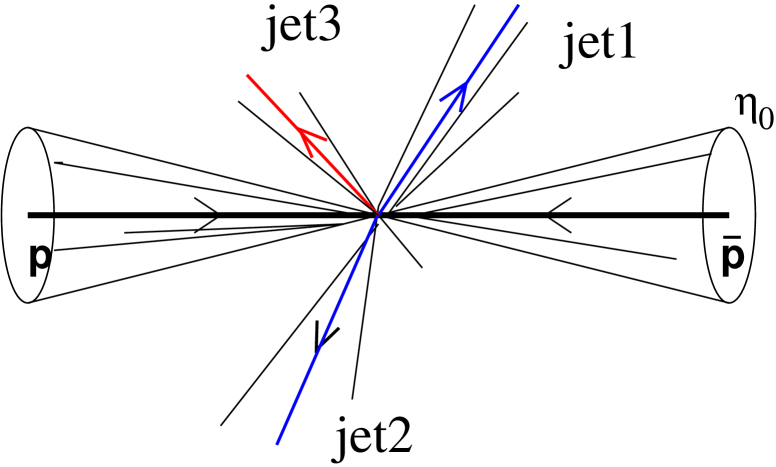
$\displaystyle\color[rgb]{0,0,1}y_{23}\ll 1$

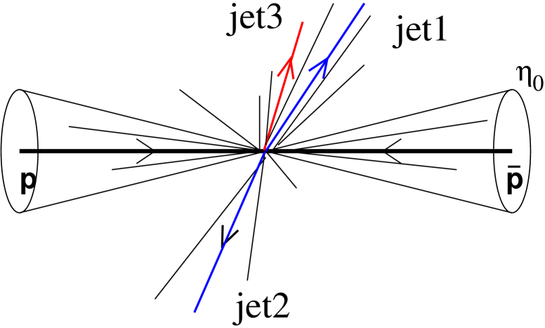
Figure 1: Illustration of a three-jet event, $y_{23}\sim 1$ (left) and of a two-jet-like event, $y_{23}\ll 1$ (right)

For directly global observables, measurements should be carried out as forward as possible (up to $\eta_{0}\sim 3.5$ at the Tevatron and $\eta_{0}\sim 5$ at the LHC). It has been shown KoutZ0 that measurements in the unobserved region are negligible at NLL as long as the observable is not too small. More precisely, given an observable which, in the presence of a single soft emission collinear to leg $\ell$, behaves as

$$V\sim d_{\ell}\left(\frac{k_{t}}{Q}\right)^{a}e^{-b_{\ell}\eta}g_{\ell}(\phi)\,,$$ (7)

the formal limit for NLL predictions to be valid reads

$$\ln(X\cdot V)\gtrsim-(a+b)\cdot\eta_{0}\,,\qquad b\equiv\min\{b_{1},b_{2}\}\,.$$ (8)

Here $X$ denotes a rescaling of the argument of the logarithm chosen so as to cancel the average value of $d_{\ell}g_{\ell}(\phi)$ in the resummed exponent $g_{2}({\alpha_{s}}L)$, see Dasgupta:2002dc ; Banfi:2004nk and 1,2 label the incoming legs. The strategy is then to neglect $\eta_{0}$ in theoretical predictions and to check a posteriori which portion of the tail is beyond control.

III.2 Recoil enhanced observables

The definition of recoil enhanced observables proceeds as follows: define a central region $\cal C$, e.g. $|\eta|<\eta_{\rm max}\sim{\cal O}\left({1}\right)$, which should contain the two jets, see Fig. 2. Then define central observables using particles only in the central region. For instance, the central transverse thrust is given by

$$T_{\perp,\cal C}\equiv\max_{\vec{n}_{\perp},{\cal C}}\frac{\sum_{i\in\cal C}|\vec{p}_{\perp i}\times{\vec{n}_{\perp,{\cal C}}|}}{\sum_{i\in\cal C}|\vec{p}_{\perp i}|}\,,\qquad\tau_{\perp,\cal C}\equiv 1-T_{\perp,\cal C}\,.$$ (9)

Similarly one defines a central thrust minor, or three-jet resolution variable, as in eqs. (4) and (6) but restricting the measurement to the central region.

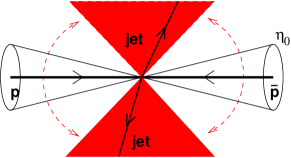
Figure 2: The central region ${\cal C}$, containing the jets, and the forward rapidity cut $\eta_{0}$.

Transverse-momentum conservation ensures that

$${\cal R}_{\perp,{\cal C}}\equiv\frac{1}{Q_{\perp,{\cal C}}}\Bigg{|}\sum_{i\in{\cal C}}{\vec{q}}_{\perp i}\Bigg{|}{=}\frac{1}{Q_{\perp,{\cal C}}}\Bigg{|}\sum_{i\not\in{\cal C}}{\vec{q}}_{\perp i}\Bigg{|}\,,\qquad Q_{\perp,{\cal C}}\equiv\sum_{i\in{\cal C}}q_{\perp i}\,.$$ (10)

Central observables can then be made global by adding the recoil term $\cal R_{\perp,\cal C}$ (or a power of it), e.g. the recoil enhanced transverse thrust, the thrust minor and the three-jet resolution parameter read

$$\tau_{\perp,\cal R}\equiv\tau_{\perp,\cal C}+{\cal R_{\perp,{\cal C}}}\>,\qquad T_{m,\cal R}\equiv T_{m,\cal C}+{\cal R_{\perp,\cal C}}\>,\qquad y_{23,\cal R}\equiv y_{23,\cal C}+{\cal R}^{2}_{\perp,\cal C}\>.$$ (11)

Note that to ensure continuous globalness Dasgupta:2002dc (roughly speaking that the transverse-momentum dependence be independent of the emission’s direction) one has to add a second power of the recoil term to $y_{23,\cal C}$.

Observables in this class are global despite the fact that measurements are truly restricted to a central region. This is because they have an indirect sensitivity to forward emissions through recoil effects. This mechanism was already well known from some DIS observables Dasgupta:2002dc .

III.3 Observables with exponentially suppressed forward terms

The last class of observables discussed is the one with exponentially suppressed forward terms. Also in this case one starts defining central observables, as in eq. (9). One then introduces the mean transverse-energy weighted rapidity $\eta_{\cal C}$ of the central region

$$\eta_{\cal C}=\frac{1}{Q_{\perp,{\cal C}}}\sum_{i\in{\cal C}}\eta_{i}\,q_{\perp i}\,,\qquad\quad$$ (12)

and defines an exponentially suppressed forward term as follows

$${\cal E}_{{\cal\bar{C}}}\equiv\frac{1}{Q_{\perp,{\cal C}}}\sum_{i\notin{\cal C}}q_{\perp i}\,e^{-|\eta_{i}-{\eta_{\cal C}}|}\,,$$ (13)

where the total transverse momentum $Q_{\perp,_{\cal C}}$ of the central region is defined in eq. (10). With these elements, one can make the usual central observables global by adding the exponentially suppressed forward term ${\cal E}_{{\cal\bar{C}}}$ (or a power of it to ensure continuous globalness). For instance, the exponentially suppressed transverse thrust, thrust minor and three-jet resolution parameter are given by

$$\tau_{\perp,\cal E}\equiv\tau_{\perp,\cal C}+{{\cal E}}_{\cal\bar{C}}\>,\qquad T_{m,\cal E}\equiv T_{m,\cal C}+{{\cal E}}_{\cal\bar{C}}\>,\qquad y_{23,\cal E}\equiv y_{23,\cal C}+{{\cal E}}^{2}_{\cal\bar{C}}\>.$$ (14)

Additionally, one can consider observables that are more suitably defined only in a restricted (central) region. One first separates the central region ${\cal C}$ into an up part ${\cal C}_{U}$, consisting of all particles in ${\cal C}$ with $\vec{p}_{\perp}\cdot\vec{n}_{T,{\cal C}}>0$, and a down part ${\cal C}_{D}$, consisting of all particles in ${\cal C}$ with $\vec{p}_{\perp}\cdot\vec{n}_{T,{\cal C}}<0$.

One then defines, in analogy to $e^{+}e^{-}$ Clavelli , the normalized squared invariant masses of the two regions:

$$\rho_{X,{\cal C}}\equiv\frac{1}{Q_{\perp,{\cal C}}^{2}}\left(\sum_{i\in{\cal C}_{X}}q_{i}\right)^{2}\,,\qquad X=U,D\,,$$ (15)

from which one can obtain a (non-global) central sum of masses and a (non-global) heavy-mass:

$$\rho_{S,{\cal C}}\equiv\rho_{U,{\cal C}}+\rho_{D,{\cal C}}\,,\qquad\quad\rho_{H,{\cal C}}\equiv\max\{\rho_{U,{\cal C}},\rho_{D,{\cal C}}\}\,,$$ (16)

together with versions that include the addition of the exponentially suppressed forward term:

$$\rho_{S,{\cal E}}\equiv\rho_{S,{\cal C}}+{\cal E}_{{\cal\bar{C}}}\,,\qquad\quad\rho_{H,{\cal E}}\equiv\rho_{H,{\cal C}}+{\cal E}_{{\cal\bar{C}}}\,.$$ (17)

This separation into up and down regions can also be used to define boost-invariant jet broadenings. One first introduces rapidities and azimuthal angles of axes for the up and down regions:

$$\eta_{X,{\cal C}}\equiv\frac{\sum_{i\in{\cal C}_{X}}q_{\perp i}\eta_{i}}{\sum_{i\in{\cal C}_{X}}q_{\perp i}}\,,\qquad\phi_{X,{\cal C}}\equiv\frac{\sum_{i\in{\cal C}_{X}}q_{\perp i}\phi_{i}}{\sum_{i\in{\cal C}_{X}}q_{\perp i}}\,,\qquad X=U,D\,,$$ (18)

and defines broadenings for the two regions:

$$B_{X,{\cal C}}\equiv\frac{1}{2Q_{\perp,{\cal C}}}\sum_{i\in{\cal C}_{X}}q_{\perp i}\sqrt{(\eta_{i}-\eta_{X,{\cal C}})^{2}+(\phi_{i}-\phi_{X,{\cal C}})^{2}}\,,\qquad X=U,D\,.$$ (19)

The central total and wide-jet broadenings are then given by

$$B_{T,{\cal C}}\equiv B_{U,{\cal C}}+B_{D,{\cal C}}\,,\qquad\quad B_{W,{\cal C}}\equiv\max\{B_{U,{\cal C}},B_{D,{\cal C}}\}\,.$$ (20)

Exponentially suppressed, global observables are then obtained by adding the forward term ${\cal E}_{{\cal\bar{C}}}$

$$B_{T,{\cal E}}\equiv B_{T,{\cal C}}+{\cal E}_{{\cal\bar{C}}}\,,\qquad B_{W,{\cal E}}\equiv B_{W,{\cal C}}+{\cal E}_{{\cal\bar{C}}}\,.$$ (21)

IV Sample NLL distributions from caesar

To illustrate different features of resummed predictions, we present here some sample distributions as obtained with caesar. We select dijet events at the Tevatron Run II regime, $\sqrt{s}=1.96$ TeV, by running the longitudinally invariant $k_{t}$ algorithm JetratesHH-CDSW and by requiring the presence of two jets in the central region ($|\eta|<0.7$), the transverse momentum of the hardest jet satisfying $E_{\perp}>\mbox{E}_{\perp,\rm min}=50\mbox{ GeV}$ (unless differently specified). We define the central region $\cal C$ $|\eta|<\eta_{\rm max}=1.1$. This ensures that the two jets are well contained in $\cal C$.

Most of the properties of distributions can be understood in terms of the coefficients $a$ and $b_{\ell}$ appearing in the parametrization of the observable given in eq. (7). This is because the leading Sudakov effect is given by

$$\Sigma(V)\sim e^{\frac{{\alpha_{s}}}{2\pi}G_{12}L^{2}+\dots}\,,\qquad\qquad G_{12}=-\frac{2}{a}\sum_{\ell}\frac{C_{\ell}}{a+b_{\ell}}\,,$$ (22)

so that it is determined only by the colour charges $C_{\ell}$ ($C_{\ell}=C_{F},C_{A}$ if parton $\ell$ is a quark/gluon) and by the values of $a$ and $b_{\ell}$. The point up to which the resummation is under NLL control, given in eq. (8), also depends on the values of $a$ and $b_{\ell}$ (although it also depends on the values of $d_{\ell}g_{\ell}(\phi)$ through $X$).

$V$	$a_{\ell}$ (inc)	$b_{\ell}$ (inc)	$a_{\ell}$ (out)	$b_{\ell}$ (out)
$\tau_{\perp,g}$	1	0	1	1
$T_{m,g}$	1	0	1	0
$y_{23,g}$	2	0	2	0

$V$	$a_{\ell}$ (inc)	$b_{\ell}$ (inc)	$a_{\ell}$ (out)	$b_{\ell}$ (out)
$\rho_{H,{\cal E}}$	1	1	1	1
$B_{W,{\cal E}}$	1	1	1	0

Table 1: Coefficients $a$ and $b_{\ell}$ for some global (left) and exponentially suppressed (right) observables as they appear in eq. (7), given for incoming and outgoing legs.

In Table 1 we report the values of the coefficients $a$ and $b_{\ell}$ for various observables as computed by caesar  (despite the presence of four legs it is sufficient to distinguish only between in/outgoing legs).

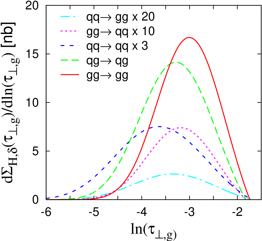
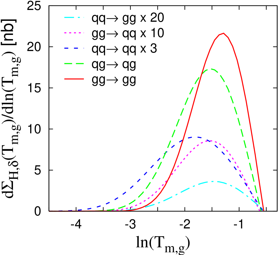
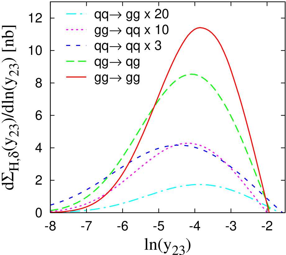
Figure 3: NLL resummed differential distributions for the directly global thrust (left), thrust minor (central) and three-jet resolution parameter (right), for various partonic channels.

In Fig. 3 we show pure NLL resummed differential distributions for various global observables, the thrust, thrust minor, and three-jet resolution parameter, defined in eqs. (3), (4), and (6) for various partonic channels. The figure shows that the thrust minor is peaked at higher values of $v$, while the peaks of $y_{23}$ lie at lowest values. This is expected since for these observables the position of the peak depends only on the coefficients of the total colour charge of in/outgoing partons, $C_{{\rm in}/{\rm out}}$ (specifically here $G_{12}=-(2C_{\rm in}+C_{\rm out}),-2(C_{\rm in}+C_{\rm out}),-(C_{\rm in}+C_{\rm out})$ for the thrust, thrust minor, and three-jet resolution, respectively). The figure also shows that tails of quark-channel distributions generally extend to lower values of $v$ compared to channels dominated by gluons. This can again be inferred from the value of $G_{12}$ for the given channel; it simply reflects the fact that quarks radiate less then gluons. The region to the left of the thick line is beyond control of the NLL resummed predictions, given in eq. (8). Note that $X\sim 5$ for the thrust, while $X=1$ for the thrust minor and $y_{23}$, so that for these last two observables the cut is located simply at $\eta_{0}$ and $2\eta_{0}$ respectively. We see that for the thrust a small part of the tail extends beyond the cut, while for the other two observables almost all the distributions are under perturbative control.

Finally, one should remark that at higher values of $v$ NLL distributions become negative. This unphysical behaviour will be corrected by the fixed-order predictions once the matching with fixed order results is carried out.

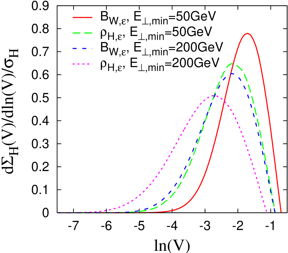
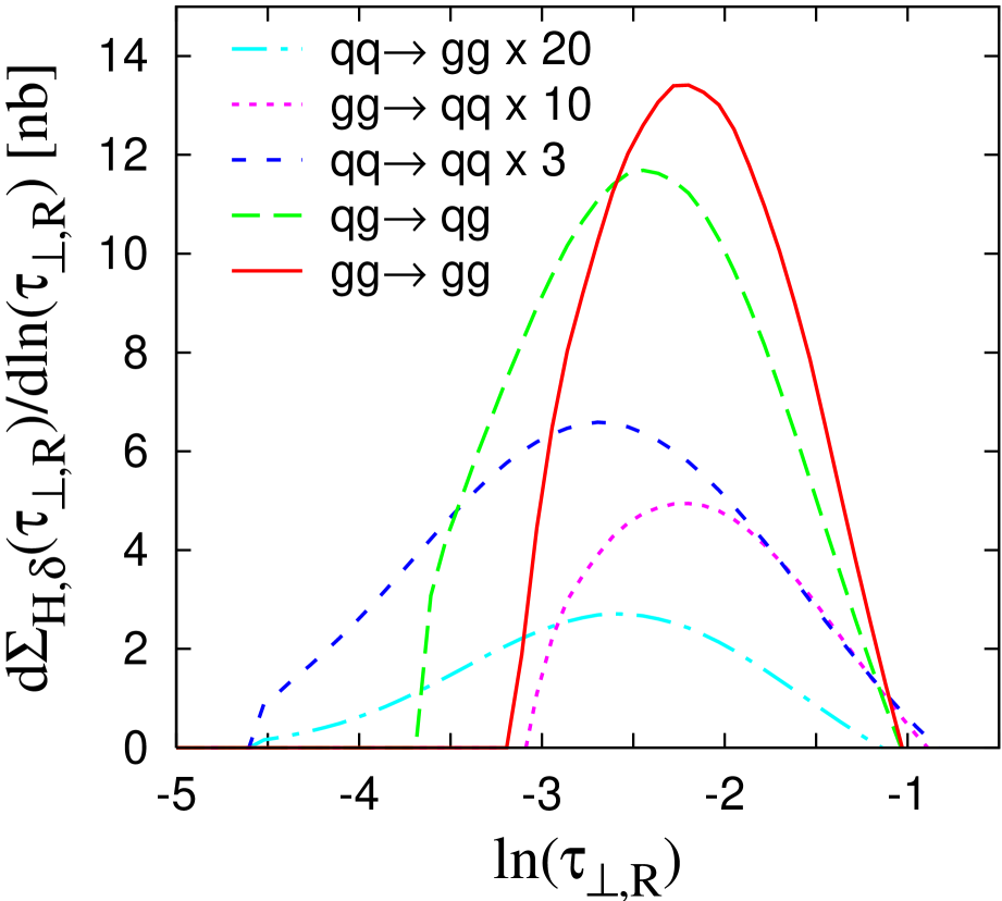
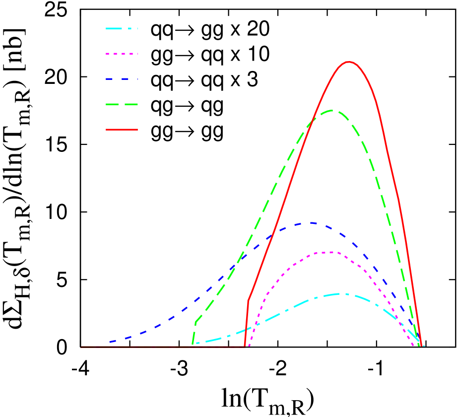
Figure 4: Total differential distribution for exponentially suppressed wide broadening and heavy jet-mass for two valued of $E_{\perp,\rm min}$ (left). Differential distributions for the recoil enhanced thrust (central) and thrust minor (right) for various partonic channels.

In Fig. 4 (left) we show total distributions, summed over all partonic channels, for two exponentially suppressed observables, a variant of the heavy jet-mass, and the wide broadening defined in eqs. (17) and (21) for two values of $E_{\perp,\rm min}$. The two observables have a different leading Sudakov suppression ($G_{12}=-(C_{\rm in}+2C_{\rm out}),-(C_{\rm in}+C_{\rm out})$ for the broadening and the jet mass respectively). Compared to directly global observables, one can see a remarkable improvement as far as the position of the cut is concerned, due to the exponentially suppressed term ($b_{\ell}=1$ for incoming legs).

One can also see the effect of changing the transverse energy cut: increasing the cut, the distribution is peaked at lower values. This is due to two different mechanisms: with higher transverse energy cuts one probes the coupling at higher scales and the parton densities at higher $x$, where quark channels become more important.

Finally, in Fig. 4 (centre and right) we show the distribution for the recoil-enhanced transverse thrust and thrust minor defined in eq. (11). Since these observable measure only very central emissions, the $\eta_{0}$ cut has no effect. However, the distributions have a different cut since the resummation breaks down at some value of $v$ (which generally depends on the channels too). This breakdown is well understood DSBroad ; RakowWebber , and it is a characteristic of all those observables for which contributions from multiple emissions can cancel one another. What happens is that, for sufficiently small $v$, it becomes more likely to suppress the value of $v$ via cancellations between emissions rather than by Sudakov suppression. This leading logarithmic (LL) change of behaviour cannot be accounted for by the NLL resummation. Points where the NLL resummation is not reliable have been excluded from the plots. The effect of this can be seen in the cut of the tails of the distributions.

V Complementarity between the observables

The above observables have complementary properties, sensitivities and advantages/disadvantages, which makes them a very rich field of activity. To be more precise, directly global observables are simple, being defined analogously to $e^{+}e^{-}$ observables, just purely in the transverse plane. However, the impact of $\eta_{0}$ is not always negligible and this can be checked only a posteriori. Observables with recoil term measure only central emissions. The recoil term can however be subject to large cancellations, making an accurate determination of it problematic. Additionally, the Sudakov effect competes with a cancellation in the vectorial sum in the recoil term, causing the resummation to break down at some point. Observables with an exponentially suppressed forward term have a very low sensitivity to the forward region; they are thus the most promising compromise. Yet experimental measurements are complicated by the fact that one needs to merge measurements from different detectors (tracking information in the central region, where a good resolution is needed, calorimeter information in the forward region, where an “average” information on the momentum flow is sufficient).

These theoretical complementarities are summarized in the first two columns of Table 2 for variants of the thrust ($\tau_{\perp}$), thrust-minor ($T_{m}$), broadenings ($B_{X}$), jet-masses ($\rho_{X}$), and three-jet resolution parameter ($y_{23}$). Additionally the table shows the sensitivity of these observables to the underlying event and the hadronization of the jets. In the following we will explain the listed properties.

Event shape	Impact of $\eta_{0}$	Resummation breakdown	Underlying event	Jet hadronization
$\tau_{\perp,g}$	tolerable∗	none	$\sim\eta_{0}/Q$	$\sim 1/Q$
$T_{m,g}$	tolerable	none	$\sim\eta_{0}/Q$	$\sim 1/(\sqrt{{\alpha_{s}}}Q)$
$y_{23}$	tolerable	none	$\sim\sqrt{y_{23}}/Q^{*}$	$\sim\sqrt{y_{23}}/Q^{*}$
$\tau_{\perp,{\cal E}}$, $\rho_{X,{\cal E}}$	negligible	none	$\sim 1/Q$	$\sim 1/Q$
$B_{X,{\cal E}}$	negligible	none	$\sim 1/Q$	$\sim 1/(\sqrt{{\alpha_{s}}}Q)$
$T_{m,{\cal E}}$	negligible	serious	$\sim 1/Q$	$\sim 1/(\sqrt{{\alpha_{s}}}Q)$
$y_{23,{\cal E}}$	negligible	none	$\sim 1/Q$	$\sim\sqrt{y_{23}}/Q^{*}$
$\tau_{\perp,{\cal R}}$, $\rho_{X,{\cal R}}$	none	serious	$\sim 1/Q$	$\sim 1/Q$
$T_{m,{\cal R}}$, $B_{X,{\cal R}}$	none	tolerable	$\sim 1/Q$	$\sim 1/(\sqrt{{\alpha_{s}}}Q)$
$y_{23,{\cal R}}$	none	intermediate∗	$\sim\sqrt{y_{23}}/Q^{*}$	$\sim\sqrt{y_{23}}/Q^{*}$

Table 2: Summary of the complementary properties of various observables. Entries marked with a * are subject to uncertainty at present.

Let us begin by considering effects of jet hadronization. Studies of $e^{+}e^{-}$ observables showed that, for those that are exponentially suppressed in rapidity, the power corrections amount to a rigid shift $\propto 1/Q$ Dokshitzer:1997iz , while those that are uniform in rapidity power corrections in addition lead to a squeeze of the distribution which is $\propto 1/(\sqrt{{\alpha_{s}}}Q)$ Dokshitzer:1998qp :

$$\begin{array}[]{lllllll}V&\sim&\frac{k_{t}}{Q}e^{-|\eta|}&\Rightarrow&\delta V^{\rm NP}&\sim&c_{V}\alpha_{0}\,\frac{\mu_{I}}{Q},\\ V&\sim&\frac{k_{t}}{Q}&\Rightarrow&\delta V^{\rm NP}&\sim&c_{V}(v)\alpha_{0}\,\frac{\mu_{I}}{\sqrt{{\alpha_{s}}}Q}.\\ \end{array}$$

The origin of the observed difference is the following. For an observable $V$, which behaves as $V\sim\frac{k_{t}}{Q}f_{V}(\eta)$, for a fixed perturbative configuration, the contribution to the power correction from parton with colour charge $C_{\ell}$ can be written schematically as

$$\delta V\sim\int_{\rm NP}\frac{dk_{\perp}}{k_{\perp}}d\eta\frac{C_{\ell}\alpha_{s}(k_{\perp})}{\pi}\frac{k_{\perp}}{Q}\,f_{V}(\eta)\,,$$ (23)

where the integration is over the region where the gluon is non-perturbative.

For observables which are exponentially damped in rapidity, the rapidity integration can be extended up to infinity. The rapidity and transverse-momentum dependence then completely factorize: the rapidity part goes into the observable dependence coefficient $c_{V}=\int d\eta f_{V}(\eta)$, while the transverse-momentum integral gives rise to $\alpha_{0}$, the average of the coupling in the IR region, below some merging scale $\mu_{I}$, given in eq. (1). One obtains

$$\delta V\propto c_{V}\alpha_{0}\,\frac{\mu_{I}}{Q}\,.$$ (24)

For observables which are uniform in rapidity, the rapidity integral cannot be extended up to infinity and PT radiation provides an effective cut-off in the rapidity integration. This cut-off is generally given by the angle between the direction of hard emissions and the reference directions used for the measurements (e.g. thrust axis in 2-jet events, event-plane for near-to-planar 3-jet events). This angle depends logarithmically on the transverse momentum of the hard emitting parton $q_{t}$. Averaging this contribution over the Sudakov PT recoil distribution $e^{-{\alpha_{s}}\ln^{2}(q_{t}/Q)}$ amounts to a singular correction $\propto 1/\sqrt{{\alpha_{s}}}$.

This same pattern is expected to hold in hadron–hadron collisions as well. The parametrization of the observable given in eq. (7), which is established automatically by caesar, allows one to determine the rapidity behaviour of the observable (i.e. the value of the $b_{\ell}$) and therefore the type of power correction. Specifically, observables with $b_{\ell}=1$ for outgoing legs will have power corrections $1/Q$, while those with $b_{\ell}=0$ for outgoing legs will have power corrections $1/(\sqrt{{\alpha_{s}}}Q)$. Finally, one sees from the table that power corrections for the $y_{23}$ jet-resolution parameters are estimated to be $\propto\sqrt{y_{23}}/Q$. The reason is that, contrary to the other observables, which are linear in $k_{t}$, $y_{23}$ is quadratic, therefore the effect of the power correction can be estimated via

$$\delta y_{23} = y_{23,\rm NP}-y_{23,\rm PT}\propto\int_{0}^{\mu_{I}}\frac{dk_{\perp,\rm NP}}{Q}d\eta\,{\alpha_{s}}(k_{\perp})\left(\frac{(k_{\perp,\rm PT}+k_{\perp,\rm NP})^{2}}{Q^{2}}-\frac{k_{\perp,\rm PT}^{2}}{Q^{2}}\right)$$ (25)

$$\sim \int_{0}^{\mu_{I}}\frac{dk_{\perp}^{\rm NP}}{Q}{\alpha_{s}}(k_{\perp})\frac{k_{\perp}^{\rm PT}k_{\perp}^{\rm NP}}{Q^{2}}\sim\sqrt{y_{23}}\alpha_{0}\frac{\mu_{I}}{Q}\,.$$ (26)

Finally, let us motivate how the underlying event affects measurements of these observables. We assume that particles from the underlying event are distributed uniformly in rapidity tube-model ; therefore the effect of the underlying event to an observable $V$, parametrized according to eq. (7), can be estimated by

$$\langle\delta^{(\rm U.E.)}V\rangle\sim\int_{{-\eta_{0}}}^{\eta_{0}}d\eta\int dk_{\perp}\frac{d\phi}{2\pi}\frac{dn^{(\rm U.E.)}}{d\eta dk_{\perp}}d_{1,2}\left(\frac{k_{\perp}}{Q}\right)^{a}e^{-b_{1/2}|\eta|}g_{1,2}(\phi)\sim\frac{\langle k_{\perp}^{a}\rangle^{(\rm U.E.)}}{Q^{a}}\langle g_{1,2}(\phi)\rangle\int_{{-\eta_{0}}}^{\eta_{0}}d\eta\,e^{-b_{1,2}|\eta|}\,.$$ (27)

If we consider observables for which $b_{\ell}=0$ for incoming legs, the underlying event will be enhanced by $\sim\eta_{0}$, while for observables with $b_{\ell}=1$, the rapidity integral can be safely extended up to infinity and the result is $\eta_{0}$-independent. For observables quadratic in $k_{\perp}$, like $y_{23}$, taking into account the interplay between PT and NP emissions amounts to an effect that is observable-dependent and goes again as $\sqrt{y_{23}}/Q$. Finally, there are observables for which there is a suppression coming from the vanishing of $\langle g_{1,2}(\phi)\rangle$. This suppression is the reason why the contribution of the underlying event does not have an $\eta_{0}$ enhancement in the case of $T_{m,{\cal E}}$, despite the fact that $b_{1/2}=0$. The different ways in which jet hadronization and underlying event affect the event shape distributions should make it possible to disentangle the two effects and study them separately.

VI Conclusions

We showed that different observables in hadron–hadron collisions have complementary sensitivities and properties. This makes them a powerful tool to investigate properties of QCD radiation, in particular the effects due to jet hadronization and to the underlying event. These studies are feasible thanks to the automated resummation tool caesar. However, before phenomenological studies can be carried out, resummed predictions need to be matched with NLO results. In hadronic collisions a channel-by-channel matching requires the flavour information Banfi:2006hf for the fixed-order predictions, which is unfortunately not currently available to an external user of hadron–hadron NLO programs NLOJET ; TriRad . Work in this direction is in progress.

- (1) S. Bethke, Nucl. Phys. Proc. Suppl. 135 (2004) 345 [arXiv:hep-ex/0407021].
- (2) S. Kluth et al., Eur. Phys. J. C 21 (2001) 199 [hep-ex/0012044] and references therein.
- (3) M. Beneke, Phys. Rept. 317 (1999) 1 [hep-ph/9807443].
- (4) M. Dasgupta and G. P. Salam, J. Phys. G 30 (2004) R143 [hep-ph/0312283].
- (5) F. Abe et al. [CDF Collaboration], Phys. Rev. D 44 (1991) 601.
- (6) I. A. Bertram [D0 Collaboration], Acta Phys. Polon. B 33 (2002) 3141.
- (7) J. Botts and G. Sterman, Nucl. Phys. B 325 (1989) 62.
- (8) S. Catani, L. Trentadue, G. Turnock and B. R. Webber, Nucl. Phys. B 407 (1993) 3.
- (9) Y. L. Dokshitzer, G. Marchesini and B. R. Webber, Nucl. Phys. B 469 (1996) 93 [hep-ph/9512336].
- (10) Y. L. Dokshitzer, G. Marchesini and G. P. Salam, Eur. Phys. J. C 1 (1999) 3 [hep-ph/9812487].
- (11) A. Banfi, G. Marchesini, Yu. L. Dokshitzer and G. Zanderighi, JHEP 0007 (2000) 002; JHEP 0105 (2001) 040 [hep-ph/0104162]; A. Banfi, G. Marchesini, G. Smye and G. Zanderighi, JHEP 0111 (2001) 066 [hep-ph/0111157].
- (12) A. Banfi, these proceedings hep-ph/0605125, and references therein.
- (13) G. P. Korchemsky and G. Sterman, Nucl. Phys. B 437 (1995) 415 [hep-ph/9411211]; G. P. Korchemsky and G. Sterman, Nucl. Phys. B 555 (1999) 335 [hep-ph/9902341]; E. Gardi and J. Rathsman, Nucl. Phys. B 609 (2001) 123 [hep-ph/0103217].
- (14) C. F. Berger and G. Sterman, JHEP 0309 (2003) 058 [hep-ph/0307394].
- (15) C. F. Berger and L. Magnea, Phys. Rev. D 70 (2004) 094010 [arXiv:hep-ph/0407024].
- (16) A. Banfi, G. P. Salam and G. Zanderighi, JHEP 0503 (2005) 073 and http://www.caesar.org.
- (17) R. D. Field [CDF Collaboration], in Proc. of the APS/DPF/DPB ’Summer Study on the Future of Particle Physics’ (Snowmass 2001) ed. N. Graf, eConf C010630 (2001) P501 [hep-ph/0201192].
- (18) M. Dasgupta and G. P. Salam, Phys. Lett. B 512 (2001) 323 [hep-ph/0104277].
- (19) A. Banfi, G. P. Salam and G. Zanderighi, JHEP 0408 (2004) 062 [hep-ph/0407287].
- (20) A. Banfi, G. Marchesini, G. Smye and G. Zanderighi, JHEP 0108 (2001) 047 [hep-ph/0106278].
- (21) M. Dasgupta and G. P. Salam, JHEP 0208 (2002) 032 [hep-ph/0208073].
- (22) L. Clavelli, Phys. Lett. B 85 (1979) 111; T. Chandramohan and L. Clavelli, Nucl. Phys. B 184 (1981) 365; L. Clavelli and D. Wyler, Phys. Lett. B 103 (1981) 383.
- (23) S. Catani, Y. L. Dokshitzer, M. H. Seymour and B. R. Webber, Nucl. Phys. B 406 (1993) 187.
- (24) M. Dasgupta and G. P. Salam, Eur. Phys. J. C 24 (2002) 213 [hep-ph/0110213].
- (25) P. E. L. Rakow and B. R. Webber, Nucl. Phys. B 187 (1981) 254.
- (26) Y. L. Dokshitzer, A. Lucenti, G. Marchesini and G. P. Salam, Nucl. Phys. B 511 (1998) 396 [Erratum-ibid. B 593 (2001) 729] [hep-ph/9707532].
- (27) R. D. Field and R. P. Feynman, Phys. Rev. D 15 (1977) 2590 Nucl. Phys. B 136 (1978) 1; R. P. Feynman, ‘Photon-hadron interactions’, W. A. Benjamin, New York (1972); B. R. Webber, in proceedings of the ‘Summer School on Hadronic Aspects of Collider Physics’, Zuoz, Switzerland, 1994, hep-ph/9411384.
- (28) A. Banfi, G. P. Salam and G. Zanderighi, hep-ph/0601139.
- (29) Z. Nagy, Phys. Rev. Lett. 88 (2002) 122003 [hep-ph/0110315].
- (30) W. B. Kilgore and W. T. Giele, hep-ph/0009193; Phys. Rev. D 55 (1997) 7183 [hep-ph/9610433].