TASI 2004 Lectures on the
Phenomenology of Extra Dimensions

Abstract

The phenomenology of large, warped, and universal extra dimensions is reviewed. Characteristic signals are emphasized rather than an extensive survey. This is the writeup of lectures given at the Theoretical Advanced Study Institute in 2004.

1 Introduction

The most exciting development in physics beyond the Standard Model in the past ten years is the phenomenology of extra dimensions. A cursory glance at the SLAC Spires “all time high” citation count confirms this crude statement. As of the close of the summer of 2005, the papers on large [1], warped [2], and universal [3] extra dimensions have garnered nearly 4000 citations among them. This also shows that the literature on extra dimensions is immense. As a consequence, I will utterly fail at being able to provide a complete reference list, and hence I apologize in advance for omissions.

Extra dimensions have been around for a long time. Kaluza and Klein postulated a fifth dimension to unify electromagnetism with gravity [4]. A closer look at this old idea reveals both its promise and problems. Imagine a Universe with five-dimensional (5-d) gravity, in which one dimension is compactified on a circle with circumference $L$. The Einstein-Hilbert action is

$$S=\int d^{5}x\sqrt{-g^{(5)}}\,M_{\star}^{3}R^{(5)}$$ (1)

where $g_{MN}^{(5)}$ is the metric and $R^{(5)}$ is the Ricci scalar for the five-dimensional spacetime, respectively. Expanding the metric about flat spacetime, $g_{MN}=\eta_{MN}+h_{MN}/(2M_{\star}^{3/2})$, the five-dimensional graviton $h_{MN}$ contains five physical components that are decomposed on $R_{4}\otimes S^{1}$ at the massless level as

$$\left(\begin{array}[]{cc}h_{\mu\nu}&A_{\mu 5}\\ A_{5\nu}&\phi\end{array}\right)$$ (2)

where $h_{\mu\nu}$ is the four-dimensional (4-d) graviton, $A_{\mu 5}$ is a massless vector field, and $\phi$ is a massless scalar field. The action reduces to

$$\int d^{4}x(M_{\star}^{3}L)R^{(4)}-\frac{1}{4}F_{\mu\nu}F^{\mu\nu}+\frac{1}{2}\partial_{\mu}\phi\partial^{\mu}\phi$$ (3)

comprising four-dimensional gravity plus a gauge field with coupling strength $g^{2}=(M_{*}L)^{-1}$, as well as a massless scalar field (with only gravitational couplings).

The remarkable finding that gauge theory could arise from a higher dimensional spacetime suitably compactified has been a tantalizing hint of how to unify gravity with the other gauge forces. As it stands, however, the original Kaluza-Klein proposal suffers from three problems:
(1) there is a gravitationally coupled scalar field $\phi$;
(2) the gauge field strength is order one only when $L^{-1}\sim M_{*}$;
(3) fermions are not chiral in five dimensions, leading to fermion “doubling” at the massless level.
Orbifolding the compactified spacetime on $S^{1}/Z_{2}$ doesn’t help, since the same operation that projects out half of the fermions also projects out the massless gauge field.

Where the original hope of Kaluza-Klein’s idea fails, string theory takes over, and I refer you to other TASI lectures and books to give you the past and present scoop on string theory (for starters, try Ref. [5]). These lectures, instead, concentrate on what the world is like if some of or all of the fields we know and love live in extra dimensions. There is some overlap between these lectures and those of Sundrum [6] and Csáki (with Hubisz and Meade) [7], however, I believe you will find that my perspective on this (and the direction given to me by the TASI 2004 organizers) is somewhat different. Hopefully it is useful!

There is one issue that I think is useful to dispense with right away, namely: Why study extra dimensions? In light of deconstruction [8, 9], one is tempted to believe everything can be studied from a purely four-dimensional view. This is certainly true of gauge theory. Does this mean we should discard extra dimensions and just consider product gauge theories? Here it useful to consider the point of view of Hill, Pokorski, Wang [9], in which they sought an effective theory of the Kaluza-Klein modes of an extra dimension. They emphasized that imposing a lattice cutoff on the extra dimensional space was tantamount to writing a product gauge theory with particular relationships among all of the couplings and masses. Perhaps an analogy to gauge theory is useful here. Imagine that you know nothing of gauge theory and just go out and measure couplings of fermions to gluons and gluons to themselves (3-point and 4-point couplings). Gradually, through careful measurement you would find that the couplings are all related, up to certain overall constants (later identified as group theory factors dependent on the representation of the fermions). These relationships would be curious, but certainly would not prevent you from writing down the low energy effective theory of the couplings of these particles. Eventually, once the couplings are established to be the same up to some experimental accuracy, you would discard the effective theory of totally separate couplings and instead just write down the QCD Lagrangian. Analogously, once the couplings and masses of Kaluza-Klein modes are measured to sufficient accuracy, one will likely cease to characterize this as “a product gauge theory with relationships among the couplings” and instead simply begin saying one has “discovered an extra dimension”.

All of this is true for both gauge theory and gravity. However, deconstructing gravity has proved more elusive, due to various issues of strong coupling that appear inevitable. I refer you to several papers [10] for discussions of this fascinating topic. Suffice to say, it is much more straightforward to understand the low energy effective theory of a compactified “physical” extra dimension rather than an extra dimension built out of multiple general coordinate invariances. Since the focus of these lectures is on phenomenology, this view is efficient, simple, and prudent.

2 Large Extra Dimensions

The renaissance of extra dimensions began with the Arkani-Hamed, Dimopoulos, and Dvali (ADD) proposal [1, 11] to lower the scale of quantum gravity to a TeV by localizing the SM to a 3+1 dimensional surface or “brane” in a higher dimensional spacetime. The extra dimensions are compactified into a large volume that effectively dilutes the strength of gravity from the fundamental scale (the TeV scale) to the Planck scale. A sketch of the setup is shown in Fig. 1.

Figure 1: Sketch of the large extra dimension ADD model worldview.

The idea that the quantum gravity scale could be lowered while the SM remain on a brane was motivated by earlier results in string theory. In particular, it was realized in string theory that the quantum gravity scale could be lowered from the Planck scale to the GUT scale [12]. Others also pursued extra dimensions opening up between the TeV scale to the GUT scale [13]. In this section, however, I will concentrate solely on the ADD model and discuss several of its important phenomenological implications.

First, let’s be explicit about the assumptions. The ADD model consists of

• $n$ extra dimensions, each compactified with radius $r$ (taken to be the same size for each dimension) on a torus with volume $V_{n}=(2\pi r)^{n}$.

• All SM fields (matter, Higgs, gauge fields) localized to a 3-brane (“SM brane”) in the bulk (“gravity only”) spacetime.

• Bulk and boundary spacetime is flat, i.e., the bulk and boundary cosmological constants vanish.

• The SM 3-brane is “stiff”; the fluctuations of the brane surface itself in the higher dimensional spacetime can be ignored (or, more technically, the brane fluctuations have masses of order the cutoff scale)

The action for this model divides into two pieces:

$$S=S_{\rm bulk}+S_{\rm brane}$$ (4)

where we are assuming for the moment that there is only one SM brane on which all of the SM fields live. Concentrate on the bulk action first, which is just the Einstein-Hilbert action for $4+n$ dimensional gravity:

$$S_{\rm bulk}=-\frac{1}{2}\int d^{4+n}x\sqrt{-g^{(4+n)}}M_{\star}^{n+2}R^{(4+n)}$$ (5)

We obviously integrate over all spacetime coordinates; hence the Lagrangian has mass dimension $D=4+n$. The higher dimensional Ricci curvature scalar $R^{(4+n)}$, formed in the usual way from two derivatives acting on the metric, having mass dimension 2. This determines the mass dimension of the coefficient of this highly relevant operator, namely $n+2$.

The line element of the bulk is

$$ds^{2}=g_{MN}^{(4+n)}dx^{M}dx^{N}$$ (6)

where we use capital letters, $M,N=0\ldots(4+n-1)$, as the indices for the bulk spacetime. Assumption (2) of the ADD model is that spacetime is flat, so we can write expand $g_{MN}$ about flat spacetime including fluctuations. For the moment, let’s only consider 4-d metric fluctuations, $h_{\mu\nu}$. Then the line element is

$$ds^{2}=\left(\eta_{\mu\nu}+h_{\mu\nu}\right)dx^{\mu}dx^{\nu}-r^{2}d\Omega^{2}_{(n)}$$ (7)

where $d\Omega_{(n)}$ are $n$-dimensional toroidal coordinates.

Given this factorization of the metric, the higher dimensional metric and Ricci scalar can be replaced with their four-dimensional ones,

$$\sqrt{-g^{(4+n)}} \rightarrow \sqrt{-g^{(4)}}$$ (8)

$$R^{(4+n)} \rightarrow R^{(4)}$$ (9)

where $g^{(4)}$ and $R^{(4)}$ implicitly depend on $h_{\mu\nu}$.

Now rewrite the higher dimensional action in terms of 4-d modes by “integrating out” the extra dimensions:

$$S_{\rm bulk} = -\frac{1}{2}M_{\star}^{n+2}\int d^{4+n}x\sqrt{-g^{(4+n)}}R^{(4+n)}$$ (10)

$$= -\frac{1}{2}M_{\star}^{n+2}\int d^{4}x\int d\Omega_{(n)}r^{n}\sqrt{-g^{(4)}}R^{(4)}$$ (11)

$$= -\frac{1}{2}M_{\star}^{n+2}(2\pi r)^{n}\int d^{4}x\sqrt{-g^{(4)}}R^{(4)}$$ (12)

The last line is the action for 4-d gravity. Matching the coefficient of the above action with the Planck scale, one obtains the famous result

$$M_{\mathrm{Pl}}^{2}=M_{\star}^{n+2}(2\pi r)^{n}\;.$$ (13)

This equation shows that our measured Planck scale is a derived quantity determined by the fundamental scale of quantum gravity, $M_{\star}$, and the volume of the extra dimensions, $V_{n}=(2\pi r)^{n}$.

What does this result mean physically? The weakness of 4-d long-distance gravity is fundamentally to due the graviton being spread rather thin across the extra dimensions with a small intersection with the SM-brane. At long distances, gravity behaves exactly as it does in 4-d by construction, since we have integrated out the extra dimensions and matched this action to the usual 4-d action. Close to the length scale of the extra dimensions, however, the gravitational potential changes and one expects to see macroscopic changes in the strength of the force of gravity.

2.1 Deviations from Newtonian Gravity

Classically, the gravitational potential changes at short distance. The Newtonian potential between two bodies of mass $m_{1}$ and $m_{2}$ is

$$V(r^{\prime}) = \left\{\begin{array}[]{lcl}\displaystyle{-G_{N}^{(4+n)}\frac{m_{1}m_{2}}{r^{\prime 1+n}}}&&r^{\prime}<r\\[10.00002pt] \displaystyle{-G_{N}\frac{m_{1}m_{2}}{r^{\prime}}}&&r^{\prime}>r\end{array}\right.$$ (16)

where $r^{\prime}$ represents the distance separating the objects, not to be confused with the size of the extra dimensions, $r$.

This leads to a vital question: How well is gravity measured? The answer is, for short distances, rather poorly compared with all the other forces. With hindsight, we really should not be surprised since gravity is so weak in comparison to the other forces. Nevertheless, it was the genius of ADD to exploit this fact in constructing their model.

For years there have been outlandish ideas on the potential modification of gravity at small but macroscopic distances, from fifth force shenanigans to light scalar moduli from certain string theories. There is some history here, and since each particular idea has a somewhat different functional dependence of the strength of gravity as a function of distance, experimentalists simplified all this by parameterizing deviations in Newton’s law as

$$V(r^{\prime})=-G_{N}^{(4)}\frac{m_{1}m_{2}}{r}\left(1+\alpha e^{-r^{\prime}/\lambda}\right)$$ (17)

The Yukawa form of the correction to Newton’s law roughly corresponds to the exchange of virtual bosons of mass $1/\lambda$, and $\alpha=1$ corresponds to gravitational strength.

Fig. 2 shows how well gravity is tested at macroscopic distances of direct relevance to the ADD model. You have all seen this graph many times, since it was showcased on the poster for this TASI school!

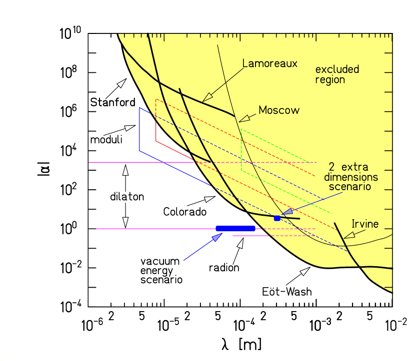
Figure 2: 95%-confidence-level constraints on ISL-violating Yukawa interactions with 1 $\mu\mathrm{m}<\lambda<1$ cm. The heavy curves give experimental upper limits. (Fig. 5 from Ref. [15].)

This is rather busy graph showing several experimental results as well as theoretical predictions for deviations in assorted models. For us, what is relevant are the experimental bounds (i.e., ignore all of the non-capitalized identifications on the graph). Five experimental results are plotted that provide the strongest constraint on deviations from Newton’s law for various ranges of distances and strengths of forces. For gravitational strength deviations, relevant to models of extra dimensions, the strongest constraint comes from the Eöt-Wash experiment that is consistent with Newtonian gravity down to about 200 microns [16]. These are remarkable experiments, and I encourage you to read the very nice review by Adelberger, Heckel and Nelson [15] for more complete details on how the experiments are done and what they imply for the assorted models that predict deviations.

How big is the deviation in the ADD model? The changeover from four-dimensional gravity to higher dimensional gravity in Eq. (16) implies that once objects are brought to a distance $r^{\prime}<r$ apart, they begin to experience a gravitational potential increasing in strength proportional to $1/r^{\prime n+1}$. Gravity becomes far stronger at short distances. Since experiment has not found any (unambiguous) deviations from the $1/r^{\prime}$ potential, the best we can do is to constrain the parameters of the ADD model using these null results.

For the ADD model, it’s obvious that $\alpha\sim 1$, $\lambda\sim r$ is where an $\mathcal{O}(1)$ deviation from Newtonian gravity is expected. Doing this a bit more carefully (for example, see [15]), one obtains

$$\lambda = r$$ (18)

$$\alpha = \frac{4}{3}(2n)$$ (19)

where $2n$ sums over the number of KK gravitons with the same mass, and the $4/3$ factor results from summing over all polarizations of the massive KK graviton.

Numerically, the size of this correction depends on the volume of the extra dimensions and the size of the fundamental Planck scale $M_{\star}$. Let’s take the lowest value that we could possibly imagine, namely $M_{\star}\sim 1$ TeV. This choice “solves” the hierarchy problem by lowering the cutoff scale of the Standard Model to 1 TeV. There are many implications of this, particularly if cutoff scale effects violate the global symmetries of the Standard Model such as flavor, baryon number, lepton number, etc. This is certainly what an effective field theorist should expect happens, and so ADD is immediately faced with serious problems. Let’s not forget, however, that every other “solution” to the hierarchy problem also faces the same problems, i.e., excess violation of SM global symmetries. (For an amusing comparison of ADD to supersymmetry, see [17].) Just as there are fixes to these model-induced problems in supersymmetry, there are also some ingenious fixes for extra dimensions, and I’ll mention a few at the end of this section and in the third lecture.

For now, let’s just calculate. Assuming equal-sized extra dimensions, we can trivially solve for the radius of $n$ extra dimensions from Eq. (13),

$$r=\frac{1}{2\pi}\left(\frac{M_{\mathrm{Pl}}^{2}}{M_{\star}^{n+2}}\right)^{1/n}\;.$$ (20)

Setting $M_{\star}=1$ TeV, here is a table of the distance scale where one expects order one deviations from Newtonian gravity:

number of extra dimensions	$r$
$n=1$	$\sim 10^{12}$ m
$n=2$	$\sim 10^{-3}$ m
$n=3$	$\sim 10^{-8}$ m
$\vdots$
$n=6$	$\sim 10^{-11}$ m

Clearly, one extra dimension $n=1$ with $M_{\star}=1$ TeV is totally ruled out by solar system tests of Newtonian gravity. It is amusing to see how well gravity really is measured at these distances. This is shown in Fig. 3,

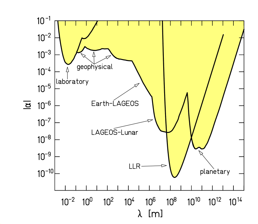
Figure 3: 95%-confidence-level constraints on ISL-violating Yukawa interactions with $\lambda>1$ cm. The LLR constraint is based on the anomalous perigee precession; the remaining constraints are based on Keplerian tests. (Fig. 4 from Ref. [15].)

where estimates of the bounds on new Yukawa-like forces are shown from a diverse set of experimental techniques across the distance scales in the figure. As an aside, notice that for distances several orders of magnitude longer than the solar system, deviations from Newtonian gravity are not well constrained. Indeed, astronomers have in fact measured very significant deviations from Newtonian gravity on galactic distance scales: the famous mismatch between the observed rotation curves with what one would expect from Newtonian gravity given the luminous mass distribution. This is of course one motivation for dark matter; for reviews, see Refs. [18, 19, 20].

For two extra dimensions, the predicted deviation from Newtonian gravity occurs at $r\sim 1$ mm. In 1998, when ADD wrote the first paper on their model, the best experimental limit on gravitational strength forces happened also to be at about 1 mm! Subsequent experiments, however, have found no deviation down to 200 microns, and thus rules out two extra dimensions with a quantum gravity scale of $M_{\star}=1$ TeV. For three or more extra dimensions, the predicted deviation from Newtonian gravity occurs at considerably smaller distances, less than ten nanometers. The experimental constraints on new forces at these distances are extremely weak, as shown in Fig. 4.

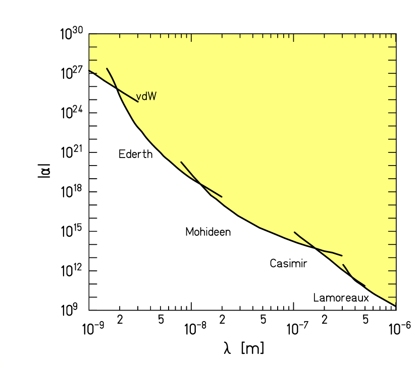
Figure 4: Constraints on ISL-violating Yukawa interactions with $1{\rm nm}<\lambda<1\mu$m. (Fig. 9 from Ref. [15].)

The good news is that ADD with $M_{\star}=1$ TeV and $n\geq 3$ is not ruled by these experiments! The bad news is that the experiments are so far from testing gravitational strength interactions that it is hopeless to attempt to observe the change from $1/r$ to $1/r^{n+1}$ directly.

2.2 Dynamics of the Higher Dimensional Graviton

Let’s generalize the line element for arbitrary metric fluctuations about a flat background bulk spacetime

$$ds^{2} = g_{MN}dx^{M}dx^{N}$$ (21)

$$= \left(\eta_{MN}+\frac{1}{2M_{\star}^{n/2+1}}h_{MN}\right)dx^{M}dx^{N}$$ (22)

where now $h_{MN}$ is the higher dimensional graviton. The coefficient is chosen for convenience to lead to canonical normalization for the graviton.

Insert the metric expansion into the higher dimensional equations of motion

$$G_{AB}\equiv R_{AB}-\frac{1}{2+n}g_{AB}R=-\frac{T_{AB}}{M_{\star}^{2+n}}$$ (23)

and one obtains [21]

$$M_{\star}^{n/2+1}G_{AB} \equiv \Box h_{AB}-\partial_{A}\partial^{C}h_{CB}-\partial_{B}\partial^{C}h_{CA}+\partial_{A}\partial^{B}h_{C}^{C}$$ (25)

$${}-\eta_{AB}\Box h_{C}^{C}+\eta_{AB}\partial^{C}\partial^{D}h_{CD}=-\frac{T_{AB}}{M_{\star}^{n/2+1}}$$

Define the higher dimensional coordinates as

$$x_{M}\equiv(x_{\mu};y_{i})\equiv(x_{0},x_{1},x_{2},x_{3};y_{1},\ldots y_{n})$$ (26)

where compactification of the extra dimensions implies the $y$’s are periodic $y_{i}\rightarrow y_{i}+2\pi r$. Upon imposing these periodic boundary conditions, the expansion of the higher dimensional graviton in terms of 4-d Kaluza-Klein fields is

$$h_{AB}(x;y)=\sum_{m_{1}=-\infty}^{\infty}\cdots\sum_{m_{n}=-\infty}^{\infty}\frac{h^{(m)}_{AB}(x)}{\sqrt{V_{n}}}e^{i\frac{m_{j}y_{j}}{r}}$$ (27)

where $h^{(m)}$ is a shorthand for $h^{(m_{1},m_{2},\ldots m_{n})}$.

The SM is confined to a 3-brane within this bulk spacetime, so that

$$T_{AB}(x;y)=\eta^{\mu}_{A}\eta^{\nu}_{B}T_{\mu\nu}\delta^{(n)}(\vec{y})$$ (28)

taking the SM brane to be located at $\vec{y}=0$. The physics content of this equation is important:

• We are neglecting brane fluctuations.

• We assume the brane is infinitely thin as represented by the $\delta$-function of extra dimensional coordinates. From an effective field theory point of view the $\delta$-function in coordinate space is unusual, potentially leading to singularities, but this can be smoothed out by replacing the $\delta$-function by $e^{-y^{2}M_{\star}^{2}}$ where the brane has a width of at least $1/M_{\star}$. Thick-brane effects can therefore be neglected so long as we work in an energy regime where $\sqrt{s}\ll M_{\star}$.

Now, plug in the KK expansion into Einstein’s equations

$$G_{\mu\nu}^{(k)}(x)= f\left(h_{\mu\nu}^{(k)},h_{\mu j}^{(k)},h^{(k)}_{jk}\right) =-\frac{T_{\mu\nu}}{M_{\mathrm{Pl}}^{2}}$$ (29)

$$G_{\mu j}^{(k)}(x)= \ldots =0$$ (30)

$$G_{jk}^{(k)}(x)= \ldots =0$$ (31)

where the precise forms of $f(\,)$ are not particularly illuminating (and can be found in [21]). Here the superscript $(k)$ refers to the Kaluza-Klein level $k$. Rewrite Einstein’s equations in terms of propagating (i.e., physical) degrees of freedom for $n\not=0$ and one obtains

$$\left(\Box+\hat{k}^{2}\right)G^{(k)}_{\mu\nu} = \frac{1}{M_{\mathrm{Pl}}}\left[-T_{\mu\nu}+\left(\frac{\partial_{\mu}\partial_{\nu}}{\hat{n}^{2}}+\eta_{\mu\nu}\right)\frac{T_{\lambda}^{\lambda}}{3}\right]$$ (32)

$$\left(\Box+\hat{k}^{2}\right)H^{(\vec{k})} = \frac{1}{2M_{\mathrm{Pl}}}\sqrt{\frac{3(n-1)}{n+2}}T_{\mu}^{\mu}$$ (33)

$$\left(\Box+\hat{k}^{2}\right)V^{(k)}_{\mu j} = 0$$ (34)

$$\left(\Box+\hat{k}^{2}\right)S^{(k)}_{jk} = 0\;$$ (35)

where the notation

$$\hat{k}^{2}\equiv\sum_{i}^{n}\left|\frac{k_{i}}{r}\right|^{2}$$ (36)

was used. The $G^{(k)}_{\mu\nu}$ correspond to massive KK gravitons that have absorbed one KK vector and one KK scalar for each KK level $k$. The $V^{(k)}_{\mu j}$ correspond to massive KK graviphotons, that absorbed one KK scalar per propagating vector per level. Finally the $S^{(k)}_{jk}$ and $H^{(\vec{k})}$ correspond to remaining massive KK scalars. At each level (for $n>1$), there is one single scalar, $H^{(\vec{k})}$, that couples to the 4-d energy momentum tensor as shown above.

These excitations are coming from the decomposition of the higher dimensional metric fluctuations

$$h_{MN}=\left(\begin{array}[]{c|ccc}h_{\mu\nu}&h_{\mu 5}&h_{\mu 6}&\ldots\\ \hline\cr&h_{55}&h_{56}&\ldots\\ &&h_{66}&\ldots\\ &&&\end{array}\right)\;.$$ (37)

Notice that the vectors and most scalars from this decomposition do not couple to SM brane-localized fields. The gravitons and $H^{(\vec{k})}$ do! Let’s do an example of this in 5-d. The five-dimensional metric fluctuation decomposition is

$$\left(\begin{array}[]{cc}h_{\mu\nu}&h_{\mu 5}\\ &\phi\end{array}\right)$$ (38)

naively has KK models

$$\begin{array}[]{ccccccc}h_{\mu\nu}^{(0)}&h_{\mu 5}^{(0)}&\phantom{000},\phantom{000}&h_{\mu\nu}^{(1)}&h_{\mu 5}^{(1)}&\phantom{000},\phantom{000}&\ldots\\ &\phi^{(0)}&\phantom{000},\phantom{000}&&\phi^{(1)}&\phantom{000},\phantom{000}&\ldots\end{array}$$ (39)

However, a massive graviton in 4-d has five polarizations: $h_{\mu\nu}^{(1)}$ eats $h_{\mu 5}^{(1)}$ and $\phi^{(1)}$; the latter are the longitudinal components.

It’s now appropriate to go through the degree of freedom counting for gravitons. As a warmup, let’s begin with gauge theory. A general gauge field $A_{M}$ in $D$ dimensions has $D$ real components. One can always choose a gauge, such as Coulomb gauge,

$$\partial_{M}A^{M} = 0$$ (40)

reducing the number of independent components to $D-1$. One can then do a gauge transformation on $A_{M}$:

$$A_{M} \rightarrow A_{M}+\partial_{M}\chi$$ (41)

for some real function $\chi$. This gauge transformation leaves the kinetic term invariant

$$F_{MN} \rightarrow \left[\partial_{M}\left(A_{N}+\partial_{N}\chi\right)-\partial_{N}\left(A_{M}+\partial_{M}\chi\right)\right]$$ (42)

$$= F_{MN}$$ (43)

since the $\partial_{M}\partial_{N}\chi$ terms drop out. A massless, on-shell $D$-dimensional gauge field has therefore $D-2$ independent components. A mass term for the gauge field, however, is famously known not to be gauge invariant since

$$\frac{1}{2}m^{2}A_{M}A^{M} \rightarrow \frac{1}{2}m^{2}\left[A_{M}A^{M}+2A^{M}\partial_{M}\chi+\partial_{M}\chi\partial^{M}\chi\right]\;.$$ (44)

This gauge-transformed Lagrangian contains terms that are rather similar to the expansion of $D_{\mu}\phi D^{\mu}\phi$ when the minimum of $\phi$ is displaced from the origin. This is just the usual Higgs mechanism where one can suitably reinterpret the last term as a kinetic term for a scalar (Goldstone) field $\chi$ and the mixing term represents the gauge boson/scalar mixing that gives rise to a gauge boson mass. A massive, on-shell gauge field in $D$ dimensions therefore has $D-1$ independent components.

The story for the graviton is entirely analogous. A $D$-dimensional graviton is a $D\times D$ real symmetric matrix with two indices, and therefore $D(D+1)/2$ components. We can first choose a gauge, such as the harmonic gauge,

$$\partial_{M}h^{M}_{N} = \frac{1}{2}\partial_{N}h^{M}_{M}$$ (45)

which reduces the number of independent components by $D$ since Eq. (45) represents $D$ independent constraints. One can then do a general coordinate transformation on $h_{MN}$:

$$h_{MN} \rightarrow h_{MN}+\partial_{M}\epsilon_{N}+\partial_{N}\epsilon_{M}$$ (46)

for some real vector function $\epsilon_{N}$. This gauge transformation leaves the kinetic term for gravity invariant. To show this, one needs the graviton kinetic term, namely the Einstein-Hilbert action expanded to leading order in the graviton fluctuation $h_{MN}$ [21]

$$R = -\frac{1}{2}h^{AB}\Box h_{AB}+\frac{1}{2}h^{A}_{A}\Box h^{B}_{B}-h^{AB}\partial_{A}\partial_{B}h^{C}_{C}+h^{AB}\partial_{A}\partial_{C}h^{C}_{B}\;.$$ (47)

I leave it as an exercise to verify that $R$ is invariant under the general coordinate transformation Eq. (46). A massless, on-shell $D$-dimensional graviton has therefore $D(D-3)/2$ independent components. For $D=4$ we obtain two real components, consistent with our expectations. A mass term for the graviton field, however, is not gauge invariant with respect to general coordinate invariance. The Fierz-Pauli graviton mass term in $D$ dimensions is

$$\frac{1}{2}m^{2}\left(h_{MN}h^{MN}-h_{M}^{M}h_{N}^{N}\right)$$ (48)

picks up non-zero contributions that include terms like $h_{MN}\partial^{M}\epsilon^{N}$. Just like for the gauge theory example above, one can suitably reinterpret the terms of the gauge transformed Fierz-Pauli action as analogous to a Higgs mechanism for gravity, where now graviton-vector mixing is the analogue of vector-scalar mixing we found above. Doing this analysis carefully, one finds that the vector is itself composed of a Goldstone (massless) vector with a Goldstone scalar, contributing a total $D-1$ components to the graviton. A massive graviton in $D$ dimensions therefore contains $D(D-1)/2-1$ components. For example, this evaluates to 5 components for a 4-d graviton, matching our expectations. A nice description of how massive gravitons absorbs vectors, the issues surrounding massive gravity (vDVZ discontinuity [22], etc.), and what this means for a deconstruction of gravity can be found in Ref. [10].

The potentially dangerous mode is the scalar degree of freedom that couples to the energy momentum tensor: the radion. The radion is a conformally-coupled scalar, and thus couples to explicit conformal violation in the Standard Model, for example

$$T_{\mu}^{\mu}\sim M_{W}^{2}W_{\mu}^{+}W^{\mu-}+m_{f}\overline{f}f+\ldots\;.$$ (49)

We have implicitly assumed that a stabilization mechanism is in place to fix the size of the extra dimensions and thus give the radion a mass sufficiently heavy so as to not modify gravity in experimentally unacceptable ways. This is obviously a highly model-dependent statement, and several groups have explored constraints on radion couplings in large extra dimension scenarios (for example, see Refs. [23, 24, 25]).

At this point, what I have done is to show you that the effects of large extra dimensions (suitably stabilized) is reduced to the problem of determining the effects of the KK modes of the graviton. Given the results thus far, it is straightforward to derive the Feynman rules. I’ll simply sketch the well known procedure for obtaining the interactions of the KK models with matter. The graviton couples to the energy momentum tensor, which we obtain from the SM action by

$$-2\frac{1}{\sqrt{-g}}\frac{\delta S_{\rm SM}}{\delta g_{\mu\nu}}=T^{\mu\nu}_{\rm SM}$$ (50)

For example, the QED part of the energy-momentum tensor is

$$T^{\mu\nu}_{\rm QED} = -F^{\mu\lambda}F_{\lambda}^{\nu}+\frac{1}{4}\eta^{\mu\nu}F^{\lambda\rho}F_{\lambda\rho}$$ (51)

The Feynman rules follow directly (for example, see [21, 27]). A few of them are shown in Fig. 5.

Figure 5: Some of the Feynman rules connecting gravitons to SM fields, from Ref. [21]. Here $W^{(f)}_{\mu\nu}=(p_{1}+p_{2})_{\mu}\gamma_{\nu}$ and the other kinematical functions $W^{(\gamma)}_{\mu\nu\alpha\beta}$ and $K(p_{1},p_{2},p_{3})_{\mu\nu\alpha\beta\gamma}$ can be found in [21]. Rules (b) and (c) are present for all SM groups; rule (d) occurs for non-Abelian groups (gluons shown).

Given the Feynman rules, we are now ready to do phenomenology!

2.3 Scales and Graviton Counting

KK gravitons have a mass $k/r$ so that the mass splittings between KK gravitons is

$$\Delta m\sim\frac{1}{r}=2\pi M_{\star}\left(\frac{M_{\star}}{M_{\mathrm{Pl}}}\right)^{2/n}\;.$$ (52)

Plugging in some numbers to give some feeling for the size

$$\Delta m\sim\left\{\begin{array}[]{lcl}0.003\;\mbox{eV}&&$n=2$\\ 0.1\;\mbox{MeV}&&$n=4$\\ 0.05\;\mbox{GeV}&&$n=6$\end{array}\right.\qquad\mbox{for}\;M_{\star}=1\;\mbox{TeV.}$$ (53)

Obviously this is very small! For illustration, the KK mass spectrum of gravitons for $n=2$ extra dimensions is shown in Fig. 6.

Figure 6: The mass spectrum of the KK gravitons is shown for $n=2$. Notice that the density of KK states fills in the energy axis quite rapidly, allowing us to very accurately replace the discrete set of KK states with a continuum.

It is convenient to replace the sum over modes with an integral over the density of states. Fig. 6 graphically shows that the continuum rapidly becomes an excellent approximation, so long as experiments are not sensitive to the mass splitting. (This is certainly true for $M_{\star}$ near the TeV scale and the number of extra dimensions is, say, $n\lesssim 6$.) The number of states $dN$ in an $n$-dimensional spatial volume having Kaluza-Klein index between $|k|$ to $|k|+dk$ is

$$dN=S_{n-1}|k|^{n-1}dk\qquad S_{n-1}=\frac{2\pi^{n/2}}{\Gamma(n/2)}$$ (54)

where $S_{n-1}$ is the area of an $n$-sphere. Using $m=|k|/r$, the density of states is

$$dN=S_{n-1}r^{n}m^{n-1}dm$$ (55)

so that the differential cross section for inclusive graviton production becomes

$$\frac{d^{2}\sigma}{dtdm}=S_{n-1}\frac{M_{\mathrm{Pl}}^{2}}{(2\pi)^{n}M_{\star}^{n+2}}m^{n-1}\frac{d\sigma_{m}}{dt}$$ (56)

where $t=(p_{1}-p_{3})^{2}$; $d\sigma/dt$ is the differential cross section for a single graviton of mass $m$; and I have substituted for $r$ using Eq. (52).

This general formula can applied to any specific process involving gravitons. For example, consider real graviton production in association with photons, $f\overline{f}\rightarrow\gamma G$. Gravitons produced at colliders in models with large extra dimensions escape the detector, leading to a missing energy. Since missing energy by itself leads to no signal at any collider detector, adding a photon to the final state allows for “tagging” of large missing energy using the single photon signal. The differential cross section to produce a particular graviton is

$$\frac{d\sigma_{m}}{dt}\left(f\overline{f}\rightarrow\gamma G\right)=\frac{\alpha Q_{f}^{2}}{16N_{f}}\frac{1}{sM_{\mathrm{Pl}}^{2}}F_{1}\left(\frac{t}{s},\frac{m^{2}}{s}\right)$$ (57)

where $\alpha$ is the photon coupling, $Q_{f}$ is the electric charge of the fermion, $N_{f}$ is number of colors, and $s$ is the center of mass energy. Using the Feynman rules given above, the kinematical function $F_{1}(x,y)$ can be computed, and is given in the Appendix of Ref. [21]. Notice that the cross section for producing a single graviton is suppressed by the 4-d Planck scale, as you would expect. But upon integrating over the huge density of states from $1/r$ up to the energy of the process $\sqrt{s}$, one obtains

$$\frac{d\sigma_{m}}{dt}\left(f\overline{f}\rightarrow\gamma G\right)=\frac{\alpha Q_{f}^{2}}{16N_{f}}\frac{1}{sM_{\star}^{2+n}}S_{n-1}\frac{m^{n-1}}{(2\pi)^{n}}F_{1}\left(\frac{t}{s},\frac{m^{2}}{s}\right)$$ (58)

where the dependence on the 4-d Planck scale cancels! This of course had to happen, since we could have just as easily done the same calculation in $D$ dimensions, where the only scale in the problem is the fundamental quantum gravity scale, $M_{\star}$, which is the coupling of the $D$-dimensional graviton!

The total cross section is obtained by integrating over all angles. To give you a feeling for the size of this signal, consider the process where the initial state particles $\overline{f}f=e^{+}e^{-}$ from a 1 TeV center-of-mass energy collider (such a linear collider that is under active consideration by the high energy physics community). The result is shown in Fig. 7.

Figure 7: Total $e^{+}e^{-}\to\gamma+\mathrm{nothing}$ cross-section at a 1 TeV center-of-mass energy $e^{+}e^{-}$ collider. Here $M_{\star}=(2\pi)^{-n/(2+n)}M_{D}\sim(0.4\rightarrow 0.25)M_{D}$ for $n$ (called $\delta$ in the figure) between $(2\rightarrow 6)$. The signal from graviton production is presented as solid lines for various numbers of extra dimension ($n=2,3,4,5$). The Standard Model background for unpolarized beams is given by the upper dash-dotted line, and the background with $90\%$ polarization is given by the lower dash-dotted line. The signal and background are computed with the requirement $E_{\gamma}<450$ GeV in order to eliminate the $\gamma Z\to\gamma\bar{\nu}\nu$ contribution to the background. The dashed line is the Standard Model background subtracted signal from a representative dimension-6 operator. (Fig. 2 from Ref. [21].)

There are several things to glean from the figure. Holding the energy of the incident particles fixed (as a partonic collider does for you for free), you can see that more extra dimensions generically means a smaller signal; i.e., contrast the $n=2$ curve with the $n=5$ curve. This is easy to understand: As the number of dimensions increases, $1/r$ increases, and hence the density of graviton states per unit energy interval increases dramatically. Holding $\sqrt{s}/M_{\star}$ fixed, then, implies that the integrated density of states between $1/r$ to $\sqrt{s}$ always decreases as the number of dimensions increase. Hence, all other things considered equal, signals associated with graviton emission will always be harder to see as the number of extra dimensions increases. Also, notice in Fig. 7 that the estimated size of the SM background is rather substantial, and so one really has to get rather lucky with $M_{\star}$ awfully close to $\sqrt{s}$ to get a signal at a TeV $e^{+}e^{-}$ collider.

Hadron colliders can do much better. This subject has received enormous attention (the first few papers that performed calculations for hadron colliders are [21, 26, 27, 28]). As just one example, consider the basic partonic diagrams for the LHC that lead to graviton emission in association with one colored parton that becomes a jet in the detector. The basic subprocesses include $qg\rightarrow qG$ (which gives the largest contribution), $q\overline{q}\rightarrow gG$, and $gg\rightarrow gG$. Processes with a single quark or gluon in the final state are considered for the same reason that a single photon in the final state was considered for an $e^{+}e^{-}$ machine: the large missing energy can be “tagged” using the monojet plus missing energy signal. The resulting hadronic collider process is thus $pp\rightarrow\mbox{jet}+\hbox to0.0pt{\hbox to7.95831pt{\hfil/\hfil}\hss}E_{T}$. For a sufficiently high enough cut on the jet energy, the background from one jet plus $Z\rightarrow\overline{\nu}\nu$ can be sufficiently reduced to weed out the signal. Doing the calculation in detail [21] one finds the cut on the jet energy must be in the several hundred GeV to TeV range. As an illustration of the size of this process in comparison to background, Fig. 8 shows the hadronic production cross section at leading order as a function of the lowered quantum gravity scale.

Figure 8: The total ${\rm jet}+{\rm nothing}$ cross-section versus $M_{D}$ at the LHC integrated for all $E_{T,{\rm jet}}>1$ TeV with the requirement that $|\eta_{\rm jet}|<3.0$. Here again $M_{\star}=(2\pi)^{-n/(2+n)}M_{D}\sim(0.4\rightarrow 0.25)M_{D}$ for $n$ (called $\delta$ in the figure) between $(2\rightarrow 4)$. The Standard Model background is the dash-dotted line, and the signal is plotted as solid and dashed lines for $n=2$ and $4$ extra dimensions. The “a” (“b”) lines are constructed by integrating the cross-section over $\hat{s}<M_{D}^{2}$ (all $\hat{s}$).

Another interesting signal is virtual graviton exchange. Here one now must sum over all KK gravitons exchanged, so that the amplitude contains

$$\mathcal{A} \sim \frac{1}{M_{\mathrm{Pl}}^{2}}\sum\frac{1}{s-m_{\rm KK}^{2}}$$ (59)

$$\sim \frac{s^{(n-2)/2}}{M_{\star}^{n+2}}$$ (60)

where like before, the sum over the KK modes removes the $1/M_{\mathrm{Pl}}$ suppression in favor of $1/M_{\star}$ suppression. This result, unlike the real graviton emission in association with photons discussed above, has certain theoretical ambiguities.

The central issue is the positive power of $\sqrt{s}$ in the numerator. This means that this process is ostensibly diverging as one approaches $M_{\star}$. This is analogous to what happens to the amplitude of gauge boson scattering in the Standard Model without a Higgs boson. Unlike the SM, however, we don’t know what regulates quantum gravity (even if there are extra dimensions), and so this amplitude could well be affected by the UV physics that smoothes out quantum gravity (strings at a TeV!). In effective field theory, this UV dependence corresponds to higher dimensional operators suppressed by the cutoff scale, i.e., the quantum gravity scale. Hence, another way to probe the ADD model is to look for effects of these higher dimensional operators. At dimension-8, one can write the effective operator corresponding to virtual graviton exchange at tree-level

$$\frac{c}{M_{\star}^{4}}\frac{1}{2}\left(T_{\mu\nu}T^{\mu\nu}-\frac{1}{n+2}T_{\mu}^{\mu}T_{\nu}^{\nu}\right)$$ (61)

where the coefficient $c\sim 4\pi$ is conventionally taken as the strength of this operator at strong coupling using naive dimensional analysis (NDA). At dimension-6, graviton loops can also induce new four-fermion operators, of the form

$$c\frac{\overline{f}f\overline{f}f}{M_{\star}^{2}}$$ (62)

where again $c\sim 4\pi$ at strong coupling. The effects of these operators correspond to what is usually called “compositeness” in older literature, and indeed the same analysis applies. Large extra dimensions are simply one realization of these operators. The precise constraints depend on the assumption of strong coupling (the $4\pi$ coefficient) and the particular operators in question, but one finds numbers of order $1.5$ TeV for Eq. (61) and of order $15$ TeV for Eq. (62) (see 2005 update of PDG [29]).

2.4 Astrophysics

Collider experiments can probe large extra dimensions by integrating over a large number of graviton modes. To get stronger bounds one must either increase the energy of the collider or increase the luminosity. The existence of light gravitons, however, allows a different window on this physics: namely, thermal systems that are hot enough to produce graviton KK modes and large enough to produce enough of them to have an effect on the astrophysical system. Specifically, consider astrophysical systems whose temperature is

$$T\gtrsim m_{\rm KK}\;.$$ (63)

We can estimate the rate of thermal graviton production by multiplying the coupling of each graviton by the number of modes accessible,

$$\mbox{rate of graviton production}\propto\frac{1}{M_{\mathrm{Pl}}^{2}}\left(Tr\right)^{n}\sim\frac{T^{n}}{M_{\star}^{n+2}}\;.$$ (64)

To find the best astrophysical bound, we want the hottest astrophysical system in the Universe. The system must, however, be well enough understood via ordinary SM physics so that we can use it as testing laboratory. This system is a supernova, and SN1987A in particular.

SN1987A is a core collapse type II supernova that went off in our sister galaxy, the Large Magellanic Cloud, emitting a huge amount of energy mostly into neutrinos. The neutrinos appeared after the stellar core of the dying star collapsed to a neutron star and remained hot enough so that the nucleons could bremsstrahlung neutrinos via the weak interaction. Several neutrino events were recorded by underground detectors on Earth, including Kamiokande in Japan and IMB in the USA. The time extent of the neutrino burst was several seconds, suggesting the supernova remained hot enough for neutrino emission to proceed on a macroscopic time scale. The temperature of SN1987A is estimated to be $T\sim 50\pm 20$ MeV.

SN1987A has been used to constrain all sorts of non-standard physics (for example, see Ref. [30]). Here what is of most interest are the constraints on axions that have rather weak couplings to matter. The basis for constraints on axions is that too large a coupling leads to too much axion emission from the supernova that has the effect of providing a means to more rapidly cool the supernova. In this case, the time extent of neutrino observations limits the total amount of cooling, and thus the strength of the axion coupling.

Similarly, graviton emission can cause excess cooling of a supernova, and this is what we want to work out now. The calculation is a bit different between axions and gravitons, since axions are derivatively coupled. The relevant reaction for gravitons is

$$N+N\rightarrow N+N+G$$ (65)

where strong interaction effects (through pion exchange) are unsuppressed while the nucleons $N$ themselves are non-relativistic. The graviton coupling to non-relativistic matter is

$$h_{\mu\nu}T^{\mu\nu}\qquad\mbox{where}\qquad T^{\mu\nu}=\left(\begin{array}[]{cc}m&p_{i}\\ p_{i}&p_{i}p_{j}/m\end{array}\right)$$ (66)

where the transverse-traceless part couples to $p_{i}p_{j}/m\sim T$, the temperature of the non-relativistic plasma. This causes an extra suppression $T^{2}/M_{\star}^{2}$ for the cross section to produce gravitons compared with axions. The thermally averaged cross section is roughly [11]

$$\langle\sigma v\rangle\sim(30\;\mathrm{mb})\left(\frac{T}{M_{\star}}\right)^{n+2}$$ (67)

During SN collapse, roughly $10^{53}$ erg are released in a few seconds. To use this to place a bound on graviton emission, we simply require that the graviton luminosity is less than $10^{53}$ erg/s $\sim(10^{16}\;\mathrm{GeV})^{2}$. The graviton luminosity is

$$L_{G}\sim M_{\rm core}\frac{n_{N}^{2}}{\rho}(30\;\mathrm{mb})\left(\frac{T}{M_{\star}}\right)^{n+2}$$ (68)

where $n_{N}$ is the nucleon number density in the core and $\rho$ is the mass density. This calculation was done carefully in [31], obtaining the constraints

$$M_{D}\gtrsim\left\{\begin{array}[]{lcl}50\;\mathrm{TeV}&&n=2\\ 4\;\mathrm{TeV}&&n=3\\ 1\;\mathrm{TeV}&&n=4\end{array}\right.$$ (69)

where $M_{D}=(2\pi)^{n/(n+2)}M_{\star}$. There is no bound for $n>4$ since the mass splitting between the gravitons is between a few to tens of MeV, leaving a rather small range of KK gravitons that can be emitted without Boltzmann suppression.

These bounds are significant for several reasons. Perhaps the most important conclusion that can be drawn from these results becomes manifest if we translate the bounds on $M_{\star}$ into upper bounds on the size of the extra dimensions:

$$r\lesssim\left\{\begin{array}[]{lcl}10^{-4}\;\mathrm{mm}&&n=2\\ 10^{-7}\;\mathrm{mm}&&n=3\\ 10^{-8}\;\mathrm{mm}&&n=4\end{array}\right.$$ (73)

Hence, the scale where gravitational strength deviations from Newton’s law are guaranteed to be present in models of large extra dimensions is far smaller than the present experimental bound (about $0.2$ mm) and indeed much smaller than future experiments are likely able to probe (at gravitational strength).

There is a good lesson here. New physics can appear in myriad experimental situations, and one must consider all of them to obtain the best bounds on the parameters of a new physics model. Of course this is not to suggest that continued experiments probing gravitational deviations is futile, but it does mean that a deviation attributed to KK gravitons would be (apparently) inconsistent with graviton emission from SN1987A.

2.5 Cosmology

There is another constraint that I want to discuss that concerns excess cooling of another big astrophysical system: the entire Universe! The source of cooling is the same as for supernovae, namely graviton emission. In 5-d language, a 5-d graviton can be emitted into the bulk with a coupling that is suppressed by just $1/M_{\star}$. In 4-d language, the probability to emit some KK mode goes as $1/M_{\star}^{n+2}$ while the decay of a given mode goes as $1/M_{\mathrm{Pl}}$. This means for high enough temperatures in the early universe, graviton emission becomes large, and this depletes the energy of the coupled plasma causing excess cooling that would be observed by large differences in big bang nucleosynthesis (BBN).

The decay rate for a graviton into two photons is

$$\Gamma_{G\rightarrow\gamma\gamma}=\frac{m_{G}^{3}}{80\pi M_{\mathrm{Pl}}^{2}}$$ (74)

which corresponds to a decay time of

$$\tau\sim\left(10^{8}\;\mbox{Gyr}\right)\left(\frac{\mbox{MeV}}{m_{G}}\right)^{3}$$ (75)

Hence, once a graviton is produced it decouples from the thermal plasma and does not decay for a long, long time.

To extract a bound on large extra dimension models, let’s compare the ordinary Hubble expansion rate to that of cooling by gravitons. Cooling by Hubble expansion is roughly

$$\left.\frac{d\rho}{dt}\right|_{\mathrm{expansion}}\sim-3H\rho\sim-3\frac{T^{2}}{M_{\mathrm{Pl}}^{2}}\rho$$ (76)

whereas cooling by graviton emission goes as

$$\left.\frac{d\rho}{dt}\right|_{\mathrm{evaporation}}\sim\frac{T^{n}}{M_{\star}^{n+2}}$$ (77)

These rates are equal at the “normalcy” temperature, which is easily found by equating the above rates, and one obtains

$$T_{\star}=10^{\frac{6n-9}{n+1}}\;\mathrm{MeV}=\left\{\begin{array}[]{lcl}10\;\mathrm{MeV}&&n=2\\ \;\;\;\vdots&&\\ 10\;\mathrm{GeV}&&n=6\;.\end{array}\right.$$ (78)

The normalcy temperature is is the maximum reheat temperature of the Universe such that cooling by ordinary Hubble expansion dominates. The good news is that this temperature is above the temperature of BBN (about $1$ MeV), and so we do not expect BBN predictions to be modified. The bad news is that we have generally thought that the Universe was far hotter than tens of MeV to tens of GeV, for example to generate weakly interacting dark matter, baryogenesis, inflation, etc. All of these phenomena need new mechanisms that operate at low temperatures. See for example Ref. [32] for a discussion of some of these issues.

2.6 Relic Photons

Even if the Universe is reheated to a temperature that is below the normalcy temperature, many light, long-lived gravitons are produced. By themselves, the relic KK gravitons are not a nuisance, but their decay products may well be. The KK graviton decay rate into photons was given above in Eq. (74), and we see that some significant fraction of the KK gravitons (ones lighter than about 5 MeV) produced in the early Universe will have decayed by now. This excess source of keV to MeV photons contributes to the diffuse cosmic $\gamma$-ray background.

Measuring the diffuse high energy photon spectrum is an ongoing enterprise. The region of interest to us has been covered by the COMPTEL experiment’s $\gamma$-ray observations, shown (in conjunction with measurements throughout the high energy photon spectrum) in Fig. 9.

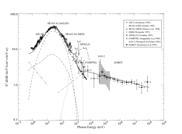
Figure 9: Multiwavelength spectrum from X-rays to $\gamma$-rays including the revised 1$\sigma$ upper limits from the Apollo experiment (Trombka 1997). The thick solid line indicates the sum of all the components. (Fig. 6 from Ref. [33].)

Since BBN requires the Universe be reheated to at least about $1$ MeV, we can obtain the best bound by requiring that the diffuse photon flux does not exceed the diffuse $\gamma$-ray observations assuming the normalcy temperature $T_{\star}=1$ MeV.

Ref. [34] worked this out, obtaining

$$\left.\frac{dn_{\gamma}}{dE}\right|_{T_{\star}=1\;\mathrm{MeV}}=\alpha_{n}(E)\left(\frac{\mathrm{TeV}}{M_{\star}}\right)^{n+2}\quad\frac{1}{\mathrm{MeV}\;\mathrm{cm}^{2}\;\mathrm{s}\;\mathrm{sr}}$$ (79)

where the coefficient was found to be

$$\alpha_{2}(4\;\mathrm{MeV}) \sim 10^{4}$$ (80)

$$\alpha_{3}(4\;\mathrm{MeV}) \sim 0.4$$ (81)

for $n=2,3$ extra dimensions evaluated at a photon energy of $4$ MeV. Comparing this result to the data allows us to extract a new bound on the quantum gravity scale

$$M_{D}>\left\{\begin{array}[]{rclcl}110&\rightarrow&350\;\mbox{TeV}&&n=2\\ 5&\rightarrow&14\;\mbox{TeV}&&n=3\end{array}\right.$$ (82)

where the first (second) number corresponds to restricting the normalcy temperature to be $1$ ($2.2$) MeV. Regardless, this is clearly the strongest bound we have seen on the scale of quantum gravity from experiment for $2$ and $3$ extra dimensions. No significant bound is obtained for $n>3$ dimensions.

3 Warped Extra Dimensions

From Sundrum’s lectures [6] and Csáki’s lectures (with Hubisz and Meade) [7] you are already well versed on warped extra dimensions. Their emphasis, however, is a bit different from the charge of these lectures. Both Sundrum and Csáki were largely interested in warped spacetimes in which some or all of the Standard Model fields propagate in the bulk. This is done for all sorts of reasons that they have expertly explained in their lectures.

In this lecture, I want to focus on the original proposal of Randall and Sundrum (RS) [2] in which only gravity exists in the warped extra dimension while the SM is confined to a 3-brane whose dimensionful parameters are scaled to the TeV scale. This is the historical approach, which may seem a bit dated by now, however I see this as a minimalist approach to general topic of warped extra dimensions: Most of what I describe below applies to these model variants involving warped extra dimensions. For instance, there are graviton resonances in the composite unification model [35] as well as the warped Higgsless model [36] as well as effects of radius stabilization, even if they are not of primary interest in those scenarios.

Without further ado, let’s plunge into the original RS model. The RS model is a 5-d theory compactified on an $S^{1}/Z_{2}$ orbifold, with bulk and boundary cosmological constants that precisely balance to give a stable 4-d low energy effective theory with vanishing 4-d cosmological constant. The basic setup is sketched in Fig. 10.

Figure 10: Sketch of the warped extra dimension RS model.

The background spacetime metric is taken to be

$$ds^{2}=e^{-k|y|}\eta_{\mu\nu}dx^{\mu}dx^{\nu}-dy^{2}$$ (83)

where the metric is not as trivial as in the ADD model. Specifically, the $y$ dependence that enters the metric as $e^{-k|y|}$ is known as the “warp factor”. The absolute value of $y$ is taken because the extra dimension is compactified on an orbifold that identifies $y\leftrightarrow-y$. We will see the physical significance of the warp factor shortly.

The action of the model is

$$S = S_{\rm bulk}+S_{\rm Planck}+S_{\rm TeV}$$ (84)

in which

$$S_{\rm bulk} = -\int d^{5}x\sqrt{-g}\left(M_{\mathrm{RS}}^{3}R-\Lambda\right)$$ (85)

$$S_{\rm Planck} = \int d^{4}x\sqrt{-g_{\rm Planck}}V_{\rm Planck}$$ (86)

$$S_{\rm TeV} = \int d^{4}x\sqrt{-g_{\rm TeV}}\left(V_{\rm TeV}+\mbox{SM Lagrangian}\right)$$ (87)

where $g_{\rm Planck}$ and $g_{\rm TeV}$ are the induced metrics on the Planck and TeV branes, respectively. Using Einstein’s equations to match the metric at $y=0,b$, one obtains

$$V_{\rm Planck} = -V_{\rm TeV}=12kM_{\mathrm{RS}}^{3}$$ (88)

$$\Lambda = -kV_{\rm Planck}$$ (89)

in terms of the AdS curvature $k$ and the fundamental quantum gravity scale $M_{\mathrm{RS}}$. This solution balances bulk curvature with boundary brane tensions (4-d cosmological constants). There is one troubling fact we see already, namely the brane tension of the TeV brane is negative. One simple way to see the effects of this is to phase rotate the entire TeV brane action, $S\rightarrow-S$, that shifts the negative sign to be in front of the kinetic terms of brane fields. Negative kinetic terms (for scalars, anyway) are well known to signal a instability in the theory in which the kinetic terms can grow (negative) arbitrarily large. We will ignore this issue here, and assume that the UV completion of the RS model stabilizes the negative tension brane (in field theory see e.g. Ref. [37] and in string theory see e.g. Ref. [38]).

Examine the SM action:

$$S_{\rm SM}=\int d^{4}x\sqrt{-g_{\rm TeV}}\left[g_{\rm TeV}^{\mu\nu}(D_{\mu}H)^{\dagger}D_{\nu}H-\lambda(H^{\dagger}H-v^{2})^{2}+\ldots\right]$$ (90)

Now insert the induced metric evaluated on the TeV brane, $(g_{\rm TeV})_{\mu\nu}=e^{-2kb}\eta_{\mu\nu}$ and one obtains

$$\int d^{4}x\left[\eta^{\mu\nu}(D_{\mu}\tilde{H})^{\dagger}(D_{\nu}\tilde{H})-\lambda\left(\tilde{H}^{\dagger}\tilde{H}-(e^{-kb}v)^{2}\right)^{2}+\ldots\right]$$ (91)

in terms of the canonically normalized fields

$$\tilde{H} = e^{-kb}H$$ (92)

$$\tilde{A}_{\mu} = e^{-kb}A_{\mu}$$ (93)

$$\tilde{f} = e^{-3kb/2}f\;.$$ (94)

The central result is that the warp factor can be rescaled away from all of the dimensionless terms of the SM (at tree-level) by field redefinitions. The only dimensionful operator, the Higgs (mass)², gets physically rescaled. We can define a new Higgs vacuum expectation value (VEV) that absorbs the warp factor

$$\tilde{v}=e^{-kb}v$$ (95)

which we see can be exponentially smaller in the canonically normalized basis.

The RS model presupposes that we take all fundamental mass parameters to be $\mathcal{O}(M_{\mathrm{Pl}})$, including $v\sim 0.1M_{\mathrm{Pl}}$. Then for a suitably large enough slice of AdS space relative to the curvature size, $kb\sim 35$, we obtain

$$\tilde{v}\sim 0.1e^{-kb}M_{\mathrm{Pl}}\sim 0.1\;\mathrm{TeV}$$ (96)

This is the key result that got everyone excited about the RS model! The interpretation is that all dimensionful parameters on the TeV brane are “warped” down to TeV scale assuming only that the size of the AdS space is parametrically larger than the inverse of the AdS curvature.

What are the sizes of fundamental parameters? The 4-d effective Planck scale can be obtained by integrating out the extra dimension to extract the coefficient of

$$\int d^{5}x\sqrt{-g^{(4)}}e^{-2k|y|}R^{(4)}$$ (97)

which is

$$M_{\mathrm{Pl}}^{2}=M_{\mathrm{RS}}^{3}\int_{y=-b}^{y=+b}e^{-2k|y|}dy=\frac{M_{\mathrm{RS}}^{3}}{k}\left(1-e^{-2kb}\right)\;.$$ (98)

Clearly, given a tiny warp factor $e^{-kb}$, all fundamental parameters can be of order the 4-d Planck scale, $M_{\mathrm{RS}}\sim k\sim M_{\mathrm{Pl}}$.

3.1 Metric Fluctuations

The generic ansatz for metric fluctuations about the RS background is

$$ds^{2}=e^{-2k|y|}g_{\mu\nu}dx^{\mu}dx^{\nu}+A_{\mu}dx^{\mu}dy-b^{2}dy^{2}\;.$$ (99)

RS is by definition an AdS spacetime on an $S^{1}/Z_{2}$ orbifold, and thus the zero mode of the graviphoton, $A_{\mu}^{(0)}$, is absent. Furthermore, we saw from ADD that in 5-d there are only graviton KK excitations since the would-be graviphoton and graviscalar KK excitations are completely absorbed into the longitudinal components of the massive KK gravitons. The mass spectrum of RS is thus exceedingly simple: the massless graviton $h_{\mu\nu}^{(0)}$, the massive KK graviton excitations $h_{\mu\nu}^{(n)}$ and a single real scalar field $\phi$, called the radion.

Consider first just the tensor excitations; for this section, I will follow closely Refs. [39, 40]. This is easiest to consider when the RS metric in written in the the conformal frame

$$ds^{2}=e^{-A(z)}\left(\eta_{\mu\nu}+h_{\mu\nu}(x,z)dx^{\mu}dx^{\nu}-dz^{2}\right)$$ (100)

with

$$e^{-A(z)}=\frac{1}{(1+k|z|)^{2}}\quad,\quad A(z)=2\log(k|z|+1)$$ (101)

where the relationship between the two coordinates is simply

$$\frac{1}{1+k|z|}=e^{-k|y|}\;.$$ (102)

We seek linearized fluctuations about the background that satisfy

$$\delta G_{MN}=\frac{1}{M_{\mathrm{RS}}^{3}}\delta T_{MN}\;.$$ (103)

First let’s fix the gauge, the “RS gauge”, in which the fluctuations satisfy $h_{\mu}^{\mu}=\partial_{\mu}h^{\mu}_{\nu}=0$. Expanding out $\delta G_{MN}$, keeping the leading order terms for $h_{\mu\nu}$, one obtains

$$-\frac{1}{2}\partial^{R}\partial_{R}h_{\mu\nu}+\frac{3}{4}\partial^{R}A\partial_{R}h_{\mu\nu} = 0\;.$$ (104)

This can be written in a somewhat cleaner way by rescaling the graviton perturbation by $h_{\mu\nu}=e^{3A/4}\tilde{h}_{\mu\nu}$ and then the linearized Einstein equations become

$$-\frac{1}{2}\partial^{R}\partial_{R}\tilde{h}_{\mu\nu}+\left[\frac{9}{32}\partial^{R}A\partial_{R}A-\frac{3}{8}\partial^{R}\partial_{R}A\right]\tilde{h}_{\mu\nu}=0\;.$$ (105)

Now separate variables

$$\tilde{h}_{\mu\nu}(x,z)=\hat{h}_{\mu\nu}(x)\phi(z)$$ (106)

where $\hat{h}$ is a four-dimensional mass eigenstate satisfying

$$\Box\hat{h}_{\mu\nu}=m^{2}\hat{h}_{\mu\nu}\;.$$ (107)

The $z$-dependence within $\phi(z)$ satisfies the 1-D Schrödinger-like equation

$$-\partial_{z}^{2}\phi+V(z)\phi=m^{2}\phi$$ (108)

where the potential can be read off from Eq. (105) to be

$$V(z)=\frac{9}{16}{A^{\prime}}^{2}-\frac{3}{4}A^{\prime\prime}$$ (109)

and primes denote derivatives with respect to $z$. Substituting for $A(z)$ using Eq. (101), one obtains

$$V(z)=\frac{15}{4}\frac{k^{2}}{(1+k|z|)^{2}}-\frac{3k}{1+k|z|}\delta(z)$$ (110)

where $V(z)$ is the famous “Volcano potential” that falls off as $1/z^{2}$ far from the UV brane with a single $\delta$-function at the caldera implying there is a single bound state (the massless 4-d graviton).

One can solve for the zero mode wavefunction

$$\phi^{(0)}(z)=e^{-3/4A(z)}\quad\Longleftrightarrow\quad\phi(y)=e^{-3/4k|y|}$$ (111)

and thus we find that the overlap of the graviton with the TeV brane is exponentially suppressed. This is why gravity appears so weak to us in the RS model. Notice that there were no small parameters needed to obtain this result, beyond the requirement of the size of the extra dimension being a factor of $35$ times the inverse of the AdS curvature.

To obtain the wavefunctions and masses of the KK modes, we first must impose boundary conditions on the 5-d graviton wavefunction:

$$\partial_{z}\phi = \left.-\frac{3}{2}k\phi\right|_{z=z_{\rm UV}}$$ (112)

$$\partial_{z}\phi = \left.-\frac{3}{2}\frac{k}{k|z|+1}\phi\right|_{z=z_{\rm IR}}$$ (113)

where $z_{\rm UV}=0$ and $z_{\rm IR}=e^{kb}/k$ are the locations of the Planck and TeV branes in the conformal coordinates. Inserting the expression for $A(z)$ into Eq. (108), we obtain

$$-\partial_{z}^{2}\phi+\frac{15}{4}\frac{k^{2}}{(k|z|+1)^{2}}=m^{2}\phi\;.$$ (114)

The solution to this PDE can be cast in terms of a sum over Bessel functions

$$\phi(z)=(kz+1)^{1/2}\left[a_{m}Y_{2}[m(z+1/k)]+b_{m}J_{2}[m(z+1/k)]\right]$$ (115)

where the boundary conditions Eqs. (112),(113) completely determine the wavefunction coefficients $a_{m},b_{m}$. The masses of the Kaluza-Klein graviton modes are easily found

$$m_{j}=x_{j}ke^{-kb}$$ (116)

where $x_{j}$ are the roots of the Bessel function $J_{1}(x_{j})=0$. Roughly,

$$x_{j}\simeq\left\{\begin{array}[]{rl}3.8&\qquad j=1\\ 7.0&\qquad j=2\\ 10.2&\qquad j=3\\ 16.5&\qquad j=4\\ &\vdots\end{array}\right.$$ (122)

where the modes are obviously not evenly spaced. Furthermore, the quantity $ke^{-kb}$ is roughly the TeV scale for a TeV brane, and thus these gravitons have masses of order the TeV scale! This is a central prediction of the RS model: distinct spin-2 resonances with a Kaluza-Klein spectrum that is spaced according to the roots of the first Bessel function.

What is the strength of the coupling of these gravitons? This is where there is a big distinction between the zero mode and the Kaluza-Klein modes of the graviton. The zero mode graviton has a $1/M_{\mathrm{Pl}}$ strength coupling, since its wavefunction is peaked near the Planck brane, while the Kaluza-Klein modes have 1/TeV strength couplings since their wavefunctions are peaked near the TeV brane. This is easy to see by simply evaluating

$$\frac{\phi(z)|_{z=z_{\rm IR}}}{\phi(z)|_{z=z_{\rm UV}}}\sim e^{kb}$$ (123)

that is exponentially enhanced by the (inverse) warp factor. Hence, the full action for the graviton fluctuations interacting with matter on the TeV brane is

$$\mathcal{L}_{\rm TeV}=-\frac{1}{M_{\mathrm{Pl}}}T^{\mu\nu}h_{\mu\nu}^{(0)}-\frac{1}{M_{\mathrm{Pl}}e^{-kb}}T^{\mu\nu}\sum_{n=1}^{\infty}h_{\mu\nu}^{(n)}\;.$$ (124)

3.2 Phenomenology of Kaluza-Klein Gravitons

We found that the Kaluza-Klein excitations of the graviton have $\mathcal{O}({\rm TeV})$ masses with $\mathcal{O}(1/{\rm TeV})$ strength couplings to fields on the TeV brane. This means that they will behave like new spin-2 resonances that can be produced and observed individually. In particular, Kaluza-Klein gravitons will decay on a timescale of order 1/TeV. This we can easily estimate on dimensional grounds to be

$$\Gamma_{G}\sim n_{\rm SM}\frac{m_{g}^{3}}{(M_{\mathrm{Pl}}e^{-kb})^{2}}$$ (125)

where $n_{\rm SM}$ is the number of SM particles into which the graviton could decay.

There are two parameters that determine the graviton production cross sections and decay rates: the warp factor and the AdS curvature. The warp factor can be equivalently replaced by the mass of the first graviton resonance. At the LHC, the $s$-channel exchange of gravitons leads to new resonances, analogous to the search for new $Z^{\prime}$ gauge bosons. The subprocesses for this include $q\overline{q},gg\rightarrow G^{(1)}\rightarrow\ell^{+}\ell^{-}$ which provides relatively clean leptonic events as well as $q\overline{q},gg\rightarrow G^{(1)}\rightarrow q\overline{q},gg$ which leads to pairs of jets that will reconstruct to the graviton mass. Using these parton processes to calculate the rate of graviton production, one can calculate a constraint on the warped Planck scale as a function of the AdS curvature. This is shown in Fig. 11, where the warped Planck scale

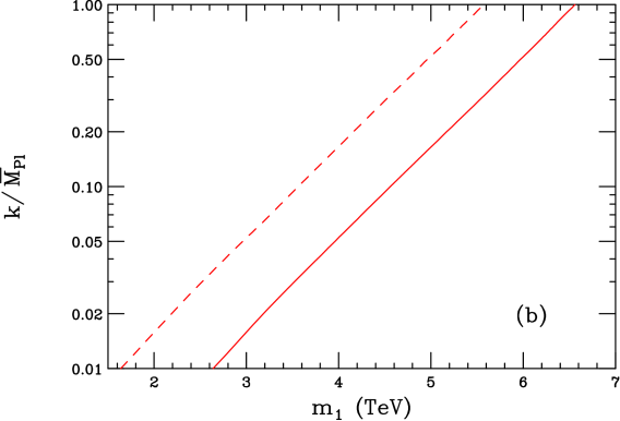
Figure 11: Exclusion regions for resonance production of the first KK graviton excitation at the the LHC. The dashed, solid curves correspond to 10, 100 fb^-1. The excluded region lies above and to the left of the curves. (Fig. 1(b) from Ref. [41].)

is related to the first graviton mass by Eq. (116). The LHC is thus able to probe to several TeV.

At a hypothetical $e^{+}e^{-}$ collider, the broad resonances of $s$-channel KK graviton exchange are clearly visible (if the energy of the collider is high enough), allowing a detailed study of the graviton properties. This is shown in Fig. 12, where an example of graviton production and

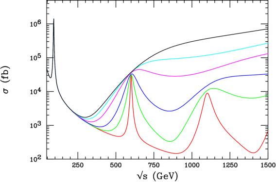
Figure 12: The cross section for $e^{+}e^{-}\to\mu^{+}\mu^{-}$ including the exchange of a tower of KK gravitons, taking the mass of the first mode to be 600 GeV, as a function of $\sqrt{s}$. From top to bottom the curves correspond to $k/M_{\mathrm{Pl}}=1.0,\,0.7,\,0.5,\,0.3,\,0.2,\,0.1$. (Fig. 2 from Ref. [41].)

decay is shown for the process $e^{+}e^{-}\rightarrow\mu^{+}\mu^{-}$ at a rather optimistic mass for the first KK resonance. In any case, the total cross section plot is rather striking!

3.3 Radius Stabilization

As it stands, the radion mass in the the RS model vanishes. This is because the brane tensions were tuned to balance the bulk cosmological constant. As there is no energy cost to increase or decrease the size of the extra dimension, radial excitations are uninhibited. This is a disaster, since massless scalar fields which couple with gravitational strength or stronger are ruled out by light-bending and other solar system tests of general relativity.

However, there is a simple modification of the original RS proposal in which dynamics can be used to stabilize the extra dimension. Goldberger and Wise realized that adding a bulk scalar field with an expectation value that had a profile, namely $v_{\rm bulk}(y)$, would be sufficient [42]. Roughly speaking, the bulk kinetic term wants to maximize the size of the extra dimension whereas the bulk mass term wants to minimize the size. The balance between these two forces results in a stabilized warped extra dimension.

A complete analysis of radius stabilization is a rather intricate affair. The original Goldberger-Wise paper [42] provides a very clear account of the problem and its solution. There are, however, a few subtleties concerning how they implemented their solution. Specifically, a naive ansatz for the radion field was used which ignores both the radion wavefunction and the backreaction of the stabilizing scalar field on the metric. This was remedied in Ref. [43] (see also Ref. [44]), were we combined the metric ansatz of Ref. [45] that solves Einstein’s equations, with a bulk scalar potential that includes backreaction effects that was given by Ref. [46]. Rather than repeating the analysis in these lectures, let me simply quote the main results here and refer interested readers to the original literature for details on the derivation.

The main properties of the radion relevant to phenomenology are its mass and couplings. The radion mass is given by

$$m_{\phi} \sim \epsilon\frac{1}{\sqrt{kb}}M_{\mathrm{Pl}}e^{-kb}$$ (126)

where $\epsilon$ is parameter that characterizes the size of the backreaction on the metric due to the bulk scalar field VEV profile. In Ref. [43], our analysis computed the mass of the radion treating the backreaction as a perturbation, and thus Eq. (126) is valid for $\epsilon\lesssim 1$. The key result here is that the radion mass is of order the warped Planck scale, i.e., the TeV scale, but parametrically smaller by a factor $1/\sqrt{kb}$. This is unlike the KK gravitons that we found above, where the first KK mode had a mass of $\simeq 4ke^{-kb}$. This suggests that the radion is the lightest mode in the RS model, and thus possibly the most important excitation to study at colliders.

The couplings of the radion to matter are also of vital importance. They were first given in [47, 48] and confirmed using the formalism described above in [43]. At leading order in the radion field, the radion couplings are

$$\frac{\phi}{\sqrt{6}M_{\mathrm{Pl}}e^{-kb}}T_{\mu}^{\mu}$$ (127)

where $T_{\mu}^{\mu}$ is the trace of the energy-momentum tensor of the Standard Model. This coupling is precisely the same as a conformally coupled scalar field, which is not surprising given the holographic interpretation of the RS model [49, 50, 51]. There is a fascinating story here, based on the AdS/CFT correspondence, concerning the duality between the 5-d RS model and a 4-d strongly-coupled conformal field theory. This would take me well beyond the scope of these lectures, and so I refer you to some excellent TASI lectures for details [52]. In any case, a phenomenologically successful RS model must have dynamics that stabilize the extra dimension and give the radion a mass, and this can be seen in either the 5-d AdS picture or the 4-d CFT dual picture.

3.4 Radion Phenomenology

Given that the radion mass, Eq. (126), is of order (slightly smaller than) the warped Planck scale, and the couplings of the radion are dimension-5 operators suppressed by the warped Planck scale, Eq. (127), the radion clearly has observable effects at high energy colliders. The mass of the radion is effectively a free parameter $m_{\phi}$, which can be bounded from above by the warped Planck scale

$$\Lambda=\sqrt{6}M_{\mathrm{Pl}}e^{-kb}$$ (128)

and bounded from below by naturalness, namely quadratically divergent radiative corrections to its mass. Roughly, then, we anticipate

$$\frac{\Lambda}{4\pi}\lesssim m_{\phi}\lesssim\Lambda$$ (129)

which corresponds to perhaps tens of GeV up to a TeV or so assuming $\Lambda\sim 1$ TeV.

The conformal couplings of the radion are straightforward to work out. The Standard Model in an unbroken electroweak vacuum, i.e., without a Higgs boson, is classically scale invariant and so $T_{\mu}^{\mu}$ vanishes classically. However, once a Higgs boson is introduced and electroweak symmetry is broken, the radion couples at tree-level to the conformal violation, namely, everywhere the Higgs VEV enters (as well as the Higgs (mass)² term). Scale invariance of the SM is broken at the quantum level, since for example coupling constants change with energy scale under the renormalization group. The radion also couples to this (loop-level) breaking of scale invariance. Thus, the tree-level couplings of the radion are identical to the Higgs boson of the SM, except that the coupling is universally scaled by a factor $v/\Lambda$. At loop-level, the scaling factor $v/\Lambda$ remains, but the coefficients change since the Higgs boson is not a conformally coupled scalar! The radion couplings, as well as the couplings of the SM Higgs boson for comparison, are shown in Fig. 13.

Figure 13: The leading order radion couplings to several fields in the Standard Model are shown. At tree-level, radion couplings are identical to Higgs boson couplings up to an overall factor $v/\Lambda$. At loop-level, the conformal couplings of the radion are manifest, for example, in the proportionality to the beta function coefficients illustrated by the coupling to gluons.

There are several comments to make about these couplings. First, the coefficient $v/\Lambda$ is expected to be of order $1/10$ for $\Lambda\sim\;{\rm TeV}$ scale. This drops out of branching ratios, and thus at tree-level the radion’s branching ratios are the same as (tree-level) Higgs branching ratios. This suggests it is rather hard to tell the radion and the Higgs apart! The definitive measure is total width: again, at tree-level we would expect $\Gamma_{\phi}=\frac{v^{2}}{\Lambda^{2}}\Gamma_{h}$. Unfortunately, measuring the total width of the Higgs boson or radion directly is somewhere between hard to really hard. How hard it is depends on the mass of the scalar in question, and thus its width, and what instruments are at our disposal. Obviously $s$-channel production at a lepton collider would be ideal, measuring the width in the same way that LEP measured the $Z$ width. The $Z$, however, has an $\mathcal{O}(1)$ coupling with the colliding leptons, whereas the Higgs and radion couple (at tree-level) with only Yukawa strength. This means an $e^{+}e^{-}$ collider is hopeless: the cross section is simply too small. A muon collider is much more promising, if such a machine could actually be made to work.

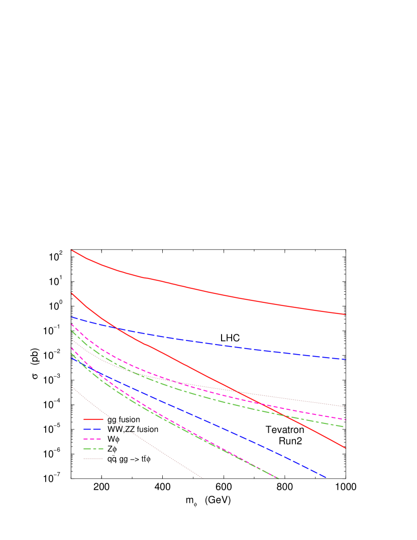
Figure 14: Production cross sections versus the mass of the radion for $p\bar{p}\to\phi$ ($gg$ fusion), $p\bar{p}\to qq^{\prime}\phi$ ($WW,ZZ$ fusion), $p\bar{p}\to W\phi$, $p\bar{p}\to Z\phi$, and $p\bar{p}\to t\bar{t}\phi$. (Fig. 3(b) from Ref. [53].)

At loop-level there are differences in the branching ratios, and fortunately the loop effects associated with the radion couplings are significant. In particular, the radion coupling to gluons has a strength that far exceeds that of the Higgs, and this has several important consequences. One is that the production cross section for radions at hadron colliders is enhanced by roughly a factor of $b_{3}^{2}=(7)^{2}$, the QCD beta function coefficient. This nearly compensates for the $v^{2}/\Lambda^{2}$ suppression factor from the conformal coupling, and leads to radion production through gluon fusion that is comparable to that of Higgs production. The production cross section for radion production at the LHC and the Tevatron is shown in Fig. 14 as a function of the radion mass.

The second effect of the large coupling to gluons is that if the radion mass is less than about $2M_{W}$, the only open decay modes are $\phi\rightarrow\overline{b}b$ and loop-level decays into gluons or photons. In the Standard Model, the Higgs branching ratio to gluons never dominates for any range of the Higgs boson mass. For radions, however, the far larger coupling to gluons dominates over the small $b$ Yukawa coupling causing the radion to decay dominantly to gluons for the radion mass range $20\;{\rm GeV}\;\lesssim m_{\phi}\lesssim 2M_{W}$. This is a strikingly different signal as compared with a Higgs boson in the same mass range. It is, in fact, a far more challenging signal to find since the two gluons become two jets, and the LHC is overwhelmed with multi-jet events with modest transverse momentum. Branching ratios for the radion into different Standard Model final states were calculated in [54, 53] and are shown in Fig. 15.

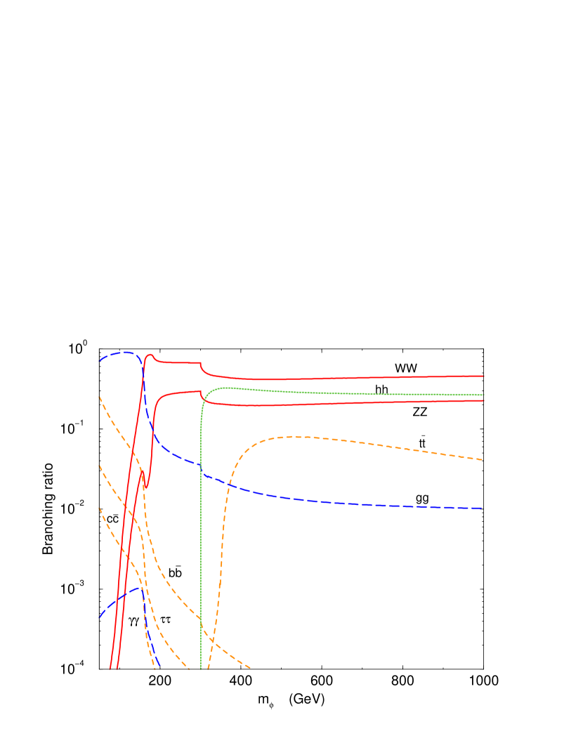
Figure 15: Branching ratios of the radion versus the radion mass. Here we have used $m_{h}=150$ GeV. (Fig. 2 from Ref. [53].)

4 Universal Extra Dimensions

4.1 Motivation

We have seen that both large and warped extra dimensions have the potential to lower the cutoff scale of the SM to the TeV scale. In ADD, we saw that the fundamental quantum gravity scale is the TeV scale, and so the TeV scale becomes the cutoff scale of the SM. In RS, identifying the cutoff scale is a bit more subtle, but the potential for phenomenological difficulties associated with higher dimensional operators remains (in the form of TeV brane-localized higher dimensional operators). This is easy to see by writing the full effective theory for the SM plus all higher dimensional operators on the TeV brane with natural size, i.e., of order the 4-d Planck scale. After the extra dimension is stabilized, the warp factor appears everywhere there is a dimensionful scale. This causes the Higgs (mass)² to warp down to the TeV scale, and simultaneously causes the higher dimensional operators proportional to $1/M_{\mathrm{Pl}}^{n}$ to scale “up” to $1/{\rm TeV}^{n}$.

In both cases, the cutoff scale is set ultimately by quantum gravity. It is well known lore that quantum gravity generically violates global symmetries (e.g., black holes with Hawking evaporation). Hence, we expect that the presence of higher dimensional operators with dimensionful coefficients of order $1/\Lambda^{n}\sim 1/({\rm TeV})^{n}$ to violate the global symmetries of the SM. The global symmetries of the SM protect against an awful lot of curious phenomena, including $B$ and $L$ violation (together or separately), non-GIM flavor symmetry violation, excessive CP violation, custodial SU(2) violation, etc. The SM relies on having a large energy desert between the weak scale and the cutoff scale to solve these problems. Experimental limits on the absence of these phenomena correspond to raising the appropriate cutoff scale of these operators high enough so that these phenomena do not occur. For instance, proton decay in the SM occurs through

$$\frac{Q\overline{Q}Q\overline{L}}{M^{2}}$$ (130)

among other dimension-6 $B$ and $L$ violating operators. On dimensional grounds, this operator leads to a proton lifetime

$$\tau\sim\frac{M^{4}}{m_{p}^{5}}$$ (131)

that must be longer than about $10^{33}$ yrs based on the super-Kamiokande bounds [55]. Converting this lifetime into a bound on the scale $M$ suppressing the operator one finds $M\gtrsim 10^{16}$ GeV.

Examples of other global symmetries of concern are:

• Lepton number violation via the dim-5 operator

  $$\frac{(HL)^{2}}{M}$$ (132)

  that leads to too large (Majorana) neutrino masses unless $M\gtrsim 10^{13}$ GeV.

• Flavor-changing neutral current (FCNC) operators, such as

  $$\frac{d\overline{s}\overline{d}s}{M^{2}}$$ (133)

  leading to excessive $K_{0}\leftrightarrow\overline{K}_{0}$ mixing.

• Baryon number violating operators, such as

  $$\frac{Qud\overline{Q}\overline{u}\overline{d}}{M^{5}}$$ (134)

  leading to neutron–anti-neutron oscillations [56].

Some of these operators, such as the one leading to $K_{0}\leftrightarrow\overline{K}_{0}$ mixing, cannot simply be forbidden by exact symmetries since this mixing has been observed experimentally and has been successfully explained by GIM-suppressed flavor violation in the SM.

There are numerous proposals for solving these problems within the contexts of the ADD model and the RS model. A small set of examples include physical separation of fermions [57], discrete symmetries [1, 58], fermions in the bulk [6], and so on. Unfortunately, I don’t have the time, space, or energy to review these ideas here. Instead, I simply want to emphasize that the ADD and RS models are incomplete as originally proposed, and require mechanisms to explain why these processes are small. Universal extra dimensions have the potential to solve some of these problems as well as provide interesting “what if” scenarios that can be tested in experiments.

4.2 UED: The Model(s)

Universal Extra Dimensions are models in which all of the SM fields live in $4+n$ dimensions with the $n$ extra dimensions taken to be flat and compact. This basic idea has a long history; for some of the earlier work see [13]. In this lecture I will primarily discuss the proposal given in [3] and then touch on several of its numerous spin-offs: a solution to the proton decay problem [59]; a rationale for three generations [60]; a test-bed for a scenario with experimental signatures that have great similarity with (versions of) supersymmetry [61, 62, 63, 64]; and a dark matter candidate [61, 65].

Promoting the full SM to extra dimensions seems like a crazy idea for several reasons. First, the spin-1/2 representations of the Poincaré group in higher dimensions generically have more degrees of freedom and differing restrictions based on chirality properties and anomalies (see Ref. [66] for a nice review). This means that fermions are generically non-chiral (with respect to our four dimensions). A simple example of this is that in five dimensions, $\gamma^{5}$ becomes part of the group structure, and so no chiral projection operators can be constructed to reduce what are intrinsically four-dimensional fermion representations to chiral two-dimensional representations. This problem is solved by “orbifolding”, i.e., compactifying on surfaces with endpoints. In five dimensions, the only choice is $S^{1}/Z_{2}$, which identifies opposite sides of a circle to create a line segment with two endpoints. In six and higher dimensions, there are many more surfaces to compactify on; the one that is more interesting for this discussion is $T^{2}/Z_{2}$.

The next problem is that gauge couplings are dimensionful. Given the higher dimensional gauge field action

$$S=\int d^{4+n}x\,F_{MN}F^{MN}$$ (135)

(where $M,N$ are the higher dimensional indices running from $0$ to $3+n$), one deduces that the canonical dimension of the gauge fields is $(2+n)/2$. This means the gauge couplings have dimension $-n/2$. Gauge field couplings in higher dimensions become analogous to graviton couplings in four dimensions, and this means these effective theories have a cutoff of order the scale of the coupling. Here I have been loose with “of order”; a more complete accounting of the relationship between the cutoff and the compactification scale can be found in Ref. [67]. I should warn you, however, that my own partially substantiated hunch is that counting $4\pi$’s in higher dimensional calculations to estimate the cutoff scale may be even more subtle. This is because if one matches these higher dimensional theories with four-dimensional product gauge theories via deconstruction, it appears that the $4\pi$ counting may be better estimated using just four-dimensional naive dimensional analysis. Anyways, for “few extra dimensional” theories, the difference is a rather innocuous $\mathcal{O}(1)$ number, and so will not really affect the discussion below.

Lastly, as good phenomenologists we will push the compactification scale to the lowest possible value that is not excluded by experiment. Putting gauge fields, fermions, and Higgs bosons in extra dimensions means there is a tower of KK excitations for all of these fields. Given that we have not seen excited massive resonances of KK photons or gluons, while colliders have probed up to the few hundred GeV scale, we can expect that $1/R\gtrsim$ hundreds of GeV. We’ll be much more precise below.

4.3 Three Generations

Dobrescu and Poppitz [60] found a very interesting result of promoting the SM into six dimensions. Six dimensions happens to be the most interesting numbers of dimensions due to existence of chiral fermions, as occurs for even numbers of dimensions, and also additional anomaly cancellation constraints, in particular due to the gravitational anomaly [68] that exists in two, six, ten, …dimensions.

The anomalies that exist in six dimensions can be classified as “irreducible” gauge anomalies, “reducible” gauge anomalies, or pure or mixed gravitational anomalies. Here “reducible” gauge anomalies correspond to most of the SM ones involving $U(1)_{Y}$ and $SU(2)_{L}$. Dobrescu and Poppitz argue that we do not need to care about anomalies associated with symmetries that are spontaneously broken. One way to rationalize this argument is that since the electroweak breaking scale and the compactification scale are roughly the same for UED, any effects associated with anomalies of these spontaneously broken gauge symmetries can be absorbed by cutoff scale effects. Alternatively, they also point out that the reducible gauge anomalies can be canceled by a higher dimensional version of the Green-Schwarz mechanism, see Ref. [60] for details.

The irreducible gauge anomalies are those associated with $SU(3)_{c}$ and $U(1)_{\rm em}$. Since colored particles and electrically charged particles are vector-like, the only non-trivial anomaly comes from $U(1)_{\rm em}[SU(3)_{c}]^{3}$ (in six dimensions, anomalies correspond to box diagrams connecting four gauge fields together).

The pure and mixed gravitational anomalies arise with respect to the six-dimensional (6-d) chirality assignments of the 6-d generalizations of SM fermions. Fermions can take on either chirality, using

$$\Gamma^{7}\cdot f \rightarrow \pm f_{\pm}$$ (136)

where $\Gamma^{M}$ are anti-commuting $2^{D/2}\times 2^{D/2}$ [$2^{(D-1)/2}\times 2^{(D-1)/2}$] matrices for even [old] $D$ dimensions. The $f_{\pm}$ are the 6-d chiral fermions (each chirality is a four-component spinor) analogous to the more familiar $f_{L,R}$ 4-d chiral fermions (where each chirality is a two-component spinor). Requiring the irreducible gauge anomaly to cancel combined with the pure and mixed gravitational anomalies leads to one of four possible 6-d chiral assignments

$$Q_{+},u_{-},d_{-},L_{+},e_{-},N_{-}$$ (137)

$$Q_{+},u_{-},d_{-},L_{-},e_{+},N_{+}$$ (138)

where the other two assignments simply flip $+\leftrightarrow-$ for all fermion species. Already, an interesting result is that a gauge-neutral fermion, $N$, is required to exist so that the pure and mixed gravitational anomaly is canceled. This requirement is curiously similar to an analogous phenomena that occurs with gauged flavor symmetry extensions of the (four-dimensional) SM [69].

Finally, there are the global gauge anomalies. These are higher dimensional analogues of the Witten anomaly for SU(2) [70]. Global gauge anomalies potentially exist for $SU(3)$, $SU(2)$, and $G_{2}$ in six dimensions. In UED, $SU(3)_{c}$ is vector-like and so automatically cancels. $SU(2)_{L}$, however, requires

$$n(2_{+})-n(2_{-})=0\;{\rm mod}\;6$$ (139)

where $n(2_{\pm})$ corresponds to the number of doublets with 6-d chirality $\pm$. For one generation, $n(Q)=3$, $n(L)=\pm 1$ implying $n(+)-n(-)=2\;{\rm or}\;4$. For $n_{g}$ generations, this becomes

$$n(Q) = 3n_{g}$$ (140)

$$n(L) = \pm n_{g}$$ (141)

$$n(2_{+})-n(2_{-}) = 2n_{g}\;{\rm or}\;4n_{g}$$ (142)

and we see that the global gauge anomaly is canceled with $n_{g}=3$ (${\rm mod}\;3$) generations!

4.4 Proton Decay

We already remarked on the potential problems with operators that lead to proton decay in models with a low cutoff scale. Ref. [59] pointed out that part of the global symmetry associated with the extra dimensional coordinates can be utilized to restrict the forms of higher dimensional operators that are allowed. In particular, in 6-d the Poincare symmetry $SO(1,5)\rightarrow SO(1,3)\times U(1)_{45}$ where the $U(1)_{45}$ corresponds to rotations between the fourth and fifth (extra dimensional) coordinates.

Chiral 6-d fermions decompose under 4-d $SU(2)_{L}$ chirality as

$$\phi_{\pm}=\phi_{\pm L}+\phi_{\pm R}$$ (143)

defined via the projection operators

$$P_{\pm L}=P_{\mp R}=\frac{1}{2}\left(1\mp\Sigma^{45}\right)$$ (144)

where $\Sigma^{\alpha\beta}/2$ are the generators of the spin-1/2 representations of $SO(1,5)$. The 4-d chiral fermions have $U(1)_{45}$ charges given by the eigenvalues of $\Sigma^{45}/2$: $\mp 1/2$ for $\phi_{\pm L}$ and $\pm 1/2$ for $\phi_{\pm R}$. This implies the $U(1)_{45}$ charge assignments for the SM fields:

fermion	$U(1)_{45}$ charge	$U(1)_{B}$
$Q_{+L}$	$-1/2$	$1/3$
$u_{-R}$, $d_{-R}$	$-1/2$	$1/3$
$L_{+L}$	$-1/2$	$0$
$e_{-R}$, $N_{-R}$	$-1/2$	$0$

Baryon number violation requires three quark fields, but obviously no combination of three quarks is invariant under $U(1)_{45}$. To obtain a $\Delta B=1$ operator, therefore, we need three lepton fields to make the operator $U(1)_{45}$-invariant. The lowest dimensional operator occurs at dimension-17

$$\mathcal{O}_{17}=\frac{\left(\overline{L}_{+L}d_{-R}\right)^{3}H^{\dagger}}{\Lambda^{11}}$$ (145)

After integrating over the extra dimensions, the 4-d low energy effective theory contains the dim-9 operator

$$\frac{v}{R^{5}\Lambda^{11}}(\overline{\nu}_{L}d_{R})(\overline{l}_{L}d_{R})^{2}$$ (146)

leading to proton decay via the 5-body process such as $p\rightarrow e^{-}\pi^{+}\pi^{+}\nu\nu$. Putting in appropriate coefficients and form factors, one obtains [59]

$$\tau_{p}\simeq 10^{35}\;\mbox{yr}\,\left(\frac{1/R}{500\;{\rm GeV}}\right)^{12}\left(\frac{\Lambda R}{5}\right)^{22}\;.$$ (147)

Hence, for $1/R$ of order the weak scale with a cutoff scale $\Lambda\gtrsim 5/R$, the 6-d UED model based on $T^{2}/Z_{2}$ is completely safe from proton decay.

One can show more generally that the sum rule

$$3\Delta B\pm\Delta L=0\;{\rm mod}\;8$$ (148)

is satisfied for all of the zero-mode fields. This forbids: proton decay with less than 6 fermions; $\Delta B=2$, $\Delta L=0$ baryon-number violating interactions leading to neutron–anti-neutron oscillations; and $\Delta B=0$, $\Delta L=2$ lepton-number violating interactions leading to Majorana neutrino masses. Hence, many of the most dangerous violations of the SM global symmetries are forbidden or sufficiently suppressed.

4.5 UED: The Model

Having piqued your interest in UED by the argument for three generations as well as naturally allowing a low cutoff scale, let’s now delve into the UED model and its phenomenology.

The action for the SM in higher dimensions is

$$S = \int d^{4}x\int d^{n}y\,\bigg{[}\frac{1}{2\overline{g}^{2}}F_{MN}F^{MN}$$ (149)

$${}+i\overline{Q}\Gamma^{M}D_{M}Q+i\overline{u}\Gamma^{M}D_{M}u+i\overline{d}\Gamma^{M}D_{M}d$$

$${}+\overline{Q}\lambda_{u}ui\sigma_{2}H^{*}+\overline{Q}\lambda_{d}dH$$

$${}+\mathcal{L}_{\rm Higgs}+\mbox{leptons}+\ldots\bigg{]}$$

where gauge interactions, Yukawa interactions, and Higgs interactions are all bulk interactions. These couplings are thus dimensionful, since this is a higher dimensional theory. In particular, it must be stressed that there are no $\delta(y)$ functions present. The UED model, by definition, has no tree-level brane-localized fields or interactions.

Demanding that all fields and interactions are bulk interactions, with no $\delta$-functions in extra-dimensional coordinate space, has one extremely important consequence. To see this, let’s first decompose a ($4+n$)-dimensional gauge field into its 4-d Kaluza-Klein (KK) components:

$$A_{\mu}(x,y) = \frac{\sqrt{2}}{(2\pi R)^{n/2}}\Bigg{\{}A_{\mu}^{(0)}(x)$$ (150)

$${}+\sqrt{2}\sum_{j_{1},\ldots,j_{n}}A_{\mu}^{(j_{1},\ldots,j_{n})}(x)\,\cos\left[\frac{j_{1}y_{1}+\ldots+j_{n}y_{n}}{R}\right]\Bigg{\}}$$

We could continue this discussion in an arbitrary number of dimensions, but for simplicity let’s concentrate on just one extra dimension. There is no loss of generality to the basic argument I am about to present by specializing to 5-d. Indeed, numerous papers that have been written about UED have concentrated on the 5-d version, so this sets us up nicely to discuss this body of work. In most cases, it is more complicated but nevertheless straightforward to extend the 5-d discussions into 6-d to preserve the properties that we found in the first two subsections.

Back to the significance of the absence of $\delta$-functions in extra-dimensional coordinate space. This is best understood with an example. Consider two distinct 5-d theories: one contains bulk fermions $F$, the other contains boundary fermions $f$ (localized at $y=0$), while both are coupled to a bulk gauge field $A_{M}$. The theory with boundary fermions has an action

$$\int d^{4}x\,dy\,\overline{f}\Gamma^{M}D_{M}f\,\delta(y)$$ (151)

that upon KK expansion becomes

$$\int d^{4}x\,dy\,\overline{f}\Gamma^{\mu}\left[A_{\mu}^{(0)}+\sqrt{2}\sum_{j}A_{\mu}^{(j)}\cos\left(\frac{jy}{R}\right)\right]f\,\delta(y)$$ (152)

where there is an overall constant as well as an additive set of interactions with the fifth component of the gauge field (an additional scalar field) that I’m not bothering about here. Integrate out the fifth dimension, assumed to be on the interval $S^{1}/Z_{2}$,

$$\int_{0}^{\pi R}dy\,\cos\left(\frac{jy}{R}\right)\delta(y)=1$$ (153)

and one is left with the 4-d Lagrangian

$$\int d^{4}x\,\overline{f}\Gamma^{\mu}\left[A_{\mu}^{(0)}+\sqrt{2}\sum_{j}A_{\mu}^{(j)}\right]f$$ (154)

where the 4-d boundary fermions couple to all of the KK modes with the same strength.

Now contrast this to what happens in the theory with only bulk fermions. The action

$$\int d^{4}x\,dy\,\overline{F}\,\Gamma^{M}D_{M}F$$ (155)

is KK expanded into

$$\int d^{4}x\,dy\,\overline{F}^{(0)}\Gamma^{\mu}\left[A_{\mu}^{(0)}+\sqrt{2}\sum_{j}A_{\mu}^{(j)}\cos\left(\frac{jy}{R}\right)\right]F^{(0)}$$ (156)

plus all of the terms with KK excitations for the fermions that I neglected to write here. Integrate out the fifth dimension

$$\frac{2}{\pi R}\int_{0}^{\pi R}dy\,\cos\left(\frac{jy}{R}\right) = 2\delta_{j0}$$ (157)

where this integral vanishes for all $j$ except $j=0$. One is left with the 4-d Lagrangian

$$\int d^{4}x\,\overline{F}^{(0)}\Gamma^{\mu}A_{\mu}^{(0)}F^{(0)}$$ (158)

where the 4-d zero mode fermions couple only to the zero mode of the gauge field! Generalizing to the $k^{\rm th}$ KK mode of one of the bulk fermions interacting with the $j^{\rm th}$ KK mode of the gauge field, the integral Eq. (157) becomes

$$\frac{2}{\pi R}\int_{0}^{\pi R}dy\,\cos\left(\frac{jy}{R}\right)\cos\left(\frac{ky}{R}\right)=\delta_{jk}$$ (159)

leading to the non-zero 4-d interactions

$$\int d^{4}x\,\overline{F}^{(k)}\Gamma^{\mu}A_{\mu}^{(k)}F^{(0)}+\overline{F}^{(0)}\Gamma^{\mu}A_{\mu}^{(k)}F^{(k)}\;,$$ (160)

also shown diagrammatically in Fig. 16.

Figure 16: Example of interactions that are allowed [(a) and (b)] and are not allowed [(c)] by KK number (or KK parity) conservation.

The presence of interactions with an even number of same-level KK modes is due precisely to the absence of $\delta$-functions. The $\delta$-functions are sources for brane-localized interactions which completely break translation invariance in the fifth dimension. The absence of $\delta$-functions implies that a discrete remnant of translation invariance survives compactification: KK number conservation.

To obtain 4-d chiral fermions, UED is compactified on an orbifold, and this introduces fixed points on which interactions that break KK number conservation could exist. Generically, KK number conservation is broken to a subgroup called KK parity [3] by brane-localized interactions that can arise radiatively [71]. The size of the one-loop brane-localized corrections for UED have been explicitly calculated in Ref. [61], which we’ll discuss more below. Nevertheless, KK parity remains unbroken so long as no explicit KK parity violating interactions are added to the orbifold fixed points. In other words, KK parity is technically natural, in that the symmetry structure is enhanced when coefficients of these bare would-be KK parity violating interactions are taken to zero. This is entirely analogous to $R$-parity in supersymmetric models.

KK parity can be written succinctly as $P_{\rm KK}=(-1)^{k}$ for the $k^{\rm th}$ KK mode. This implies:

• The lightest level-one KK mode is stable.

• Odd level KK modes can only be produced in pairs.

• Direct couplings to even KK modes occur through brane-localized, loop-suppressed interactions.

We’ll now discuss these implications of KK parity on the phenomenology of the UED model.

4.6 Corrections to Electroweak Precision Observables

The typical problem with additional gauge bosons that couple to light fermions is that they can give large contributions to electroweak precision observables. Consider the quintessential observable, the $Z$-width. Given measurements of $M_{Z}$, $G_{F}$, and $\alpha_{\rm em}(M_{Z})$, the $Z$ width can be calculated at tree-level. New contributions to the width potentially arise from the exchange of heavier gauge bosons, but such contributions do not exist in UED models since KK parity forbids tree-level couplings of $Z^{(k)}$ with the fermion zero modes as well as the $Z^{(k)}Z^{(0)}H^{(0)}{H^{(0)}}^{\dagger}$ four-point coupling.

Through one-loop interactions, however, there are calculable corrections to the electroweak precision observables. Using the parameterization given by Peskin and Takeuchi [72], the contributions to $S$ and $T$ were calculated in Ref. [3]. They found

$$T=\sum_{j}D_{j}\left(T_{j}^{t}+T_{j}^{h}+T_{j}^{V}\right)$$ (161)

where the sum is over all modes up to the cutoff scale of the $D$-dimensional theory, and $D_{j}$ is the density of states at each level $j$. The individual contributions are

$$\alpha T_{j}^{V} = -\frac{\alpha}{4\pi\cos^{2}\theta_{W}}\frac{(2n+1)M_{W}^{2}}{6M_{j}^{2}}$$ (162)

$$\alpha T_{j}^{h} = -\frac{\alpha}{4\pi\cos^{2}\theta_{W}}\frac{5m_{h}^{2}+7M_{W}^{2}}{12M_{j}^{2}}$$ (163)

$$\alpha T_{j}^{t} \simeq \frac{m_{t}^{4}}{8\pi^{2}v^{2}M_{j}^{2}}$$ (164)

where $M_{j}=j/R$ is $j^{\rm th}$ Kaluza-Klein mass level. Using the experimental values for the SM parameters, the $T$ parameter is roughly

$$T\simeq 0.76\sum_{j}D_{j}\frac{m_{t}^{2}}{M_{j}^{2}}\;.$$ (165)

A similar calculation can be done for $S$,

$$S\simeq 0.01\sum_{j}D_{j}\frac{m_{t}^{2}}{M_{j}^{2}}$$ (166)

where the contribution to the isospin-breaking parameter $T$ is two orders of magnitude larger than the isospin-preserving parameter $S$. There is no large contribution to $S$ because the heavy KK quarks acquire their mass dominantly from the vector-like contribution arising from compactification. Note that the sum over states for these electroweak parameters is

convergent $$D=5$$

log divergent for $$D=6$$

power divergent $$D>6\;.$$

Contemplating UED models with $D>6$ therefore appear somewhat problematic, since even the calculable contribution to the electroweak precision observables diverges.

In any case, using the calculable corrections we can find a lower bound on the inverse radius of the extra dimensions. Ref. [3] required the moderately loose constraint $T\lesssim 0.4$ which leads to

$$\frac{1}{R} \gtrsim \left\{\begin{array}[]{lcl}300\;\mbox{GeV}&&D=5\\ 500\;\mbox{GeV}&&D=6\;.\end{array}\right.$$ (169)

These bounds are probably a bit too low given the latest electroweak fits [29], but in any case the bound is in the several hundred GeV range. These bounds on UED dimensions should be contrasted with those that result from extra dimensions that are not universal, i.e., SM gauge bosons living in higher dimensions with SM fermions localized to 4-d. For example, Ref. [73] found constraints on the inverse size of an extra dimension of this type in the several TeV range.

4.7 UED Cutoff Scale

We have alluded to the fact that UED models are effective theories of extra dimensions with a cutoff scale. What is the cutoff scale? Since gauge couplings in extra dimensional theories are dimensionful, i.e. $\alpha_{D}$ has mass dimension $-n$, a rough guess is

$$\Lambda\sim\frac{4\pi}{\alpha_{D}^{1/n}}$$ (170)

where I have been excessively naive about my NDA counting. Matching this $D$-dimensional gauge coupling to a 4-d coupling of the SM,

$$\frac{1}{g^{2}}=\frac{(\pi R)^{n}}{g_{D}^{2}}$$ (171)

we obtain

$$\Lambda R\sim\frac{4}{\alpha^{1/n}}\sim\left\{\begin{array}[]{lcl}30&\mbox{for}&D=5\\ 10&\mbox{for}&D=6\end{array}\right.$$ (172)

which is roughly what is expected. A 4-d version of the same calculation, which is arguably better defined, sums over the number of KK particles running in loops to determine the scale of strong coupling. In this way of counting, since the number of KK modes is proportional to $n^{2}$, we would expect $\Lambda_{6-d}R\simeq\sqrt{\Lambda_{5-d}R}$, and thus $\Lambda_{6-d}R\simeq 5$. These are the typical numbers given for the cutoff scales of the 5-d and 6-d theories.

Cutoff scales that are only about one order of magnitude above the compactification scale may be problematic in other ways. While proton decay and lepton number violating operators can be suppressed or eliminated in six dimensions, given a cutoff only a factor of $5$ above the compactification scale one ought to be concerned about other higher dimensional operators that violate flavor symmetries or custodial SU(2). Also, the cutoff scale may be even lower than the above estimates suggest. Ref. [74] found that requiring scattering amplitudes satisfy the unitarity bound results in rather low estimates for the scale where strong coupling appears, only a small factor above the compactification scale.

4.8 UED in 5-d: The Spectrum

For the remainder of the discussion, I want to focus on the spectrum of the 5-d version of UED. Fortunately, the spectrum depends linearly on $1/R$ and only logarithmically on $\Lambda R$, which we will leave as a free parameter varied in some reasonable range. We will also ignore the effects of higher dimensional operators suppressed by the cutoff scale. What we will do is to examine more closely the spectrum of UED and the implications for collider searches and for the possibility of having a dark matter candidate. I’ll briefly mention the ways in which a UED dark matter candidate could be detected, emphasizing the difference from a typical supersymmetric candidate.

The spectrum of the 5-d UED model consists of all of the particles of the SM and their Kaluza-Klein excitations. Let’s focus on the first KK level. At tree-level, the masses of the KK particles are simply

$$m_{KK}^{2}=\frac{1}{R^{2}}+m_{\rm SM}^{2}$$ (173)

where $m_{SM}$ is the mass of level-zero (Standard Model) particle. This suggests a high degree of degeneracy for the KK excitations of light SM particles, but this degeneracy is not preserved beyond tree-level. Indeed, in Ref. [62] it was realized that radiative corrections to the KK particle masses are often much larger than the tree-level SM contribution.

There are two classes of calculable radiative corrections. One arises from diagrams involving bulk loops, namely particles that traverse around the circle (or actually from one side to the other, in an orbifold). The loops are non-contractable, with finite extent in the extra dimension, implying they give finite corrections to the masses. The second class of corrections involves brane-localized kinetic terms that appear on the boundaries of the orbifold. These corrections are logarithmically sensitive to the cutoff scale of the theory. The generic form of this correction to the Lagrangian is

$$\delta L = \left(\delta(y)+\delta(y-\pi R)\right)\frac{Rg^{2}}{128\pi}\ln\frac{\Lambda^{2}}{\mu^{2}}\times$$ (174)

$${}\left[\overline{F}_{+}i\hbox to0.0pt{\hbox to5.30904pt{\hfil/\hfil}\hss}\partial F_{+}+5(\partial_{5}\overline{F}_{-})F_{+}+5(\overline{F}_{+}(\partial_{5}F_{-})\right]$$

where $F_{+}$ and $F_{-}$ are the components of a bulk four-component spinor corresponding to any of the SM fermions. These corrections are necessarily logarithmically sensitive to the cutoff scale.

The shifts in the KK masses resulting from these two classes of radiative corrections are [61]:

$$\delta(m^{2}_{B^{(n)}}) = \frac{g^{\prime 2}}{16\pi^{2}R^{2}}\left(\frac{-39}{2}\frac{\zeta(3)}{\pi^{2}}-\frac{n^{2}}{3}\ln\,\Lambda R\right)$$

$$\delta(m^{2}_{W^{(n)}}) = \frac{g^{2}}{16\pi^{2}R^{2}}\left(\frac{-5}{2}\frac{\zeta(3)}{\pi^{2}}+15n^{2}\ln\,\Lambda R\right)$$

$$\delta(m^{2}_{g^{(n)}}) = \frac{g_{3}^{2}}{16\pi^{2}R^{2}}\left(\frac{-3}{2}\frac{\zeta(3)}{\pi^{2}}+23n^{2}\ln\,\Lambda R\right)$$

$$\delta(m_{Q^{(n)}}) = \frac{n}{16\pi^{2}R}\left(6g_{3}^{2}+\frac{27}{8}g^{2}+\frac{1}{8}g^{\prime 2}\right)\ln\,\Lambda R$$

$$\delta(m_{u^{(n)}}) = \frac{n}{16\pi^{2}R}\left(6g_{3}^{2}+2g^{\prime 2}\right)\ln\,\Lambda R$$

$$\delta(m_{d^{(n)}}) = \frac{n}{16\pi^{2}R}\left(6g_{3}^{2}+\frac{1}{2}g^{\prime 2}\right)\ln\,\Lambda R$$

$$\delta(m_{L^{(n)}}) = \frac{n}{16\pi^{2}R}\left(\frac{27}{8}g^{2}+\frac{9}{8}g^{\prime 2}\right)\ln\,\Lambda R$$

$$\delta(m_{e^{(n)}}) = \frac{n}{16\pi^{2}R}\frac{9}{2}g^{\prime 2}\ln\,\Lambda R\;.$$ (175)

All of the non-colored KK excitation masses are within about 10% of $m_{\gamma^{(1)}}$ up to moderately high values of the cutoff scale ($\Lambda R\approx 30$). The strongly interacting particles are somewhat heavier, up to perhaps $20\%-25\%$ above $1/R$. Fig. 17 gives an example of this spectrum

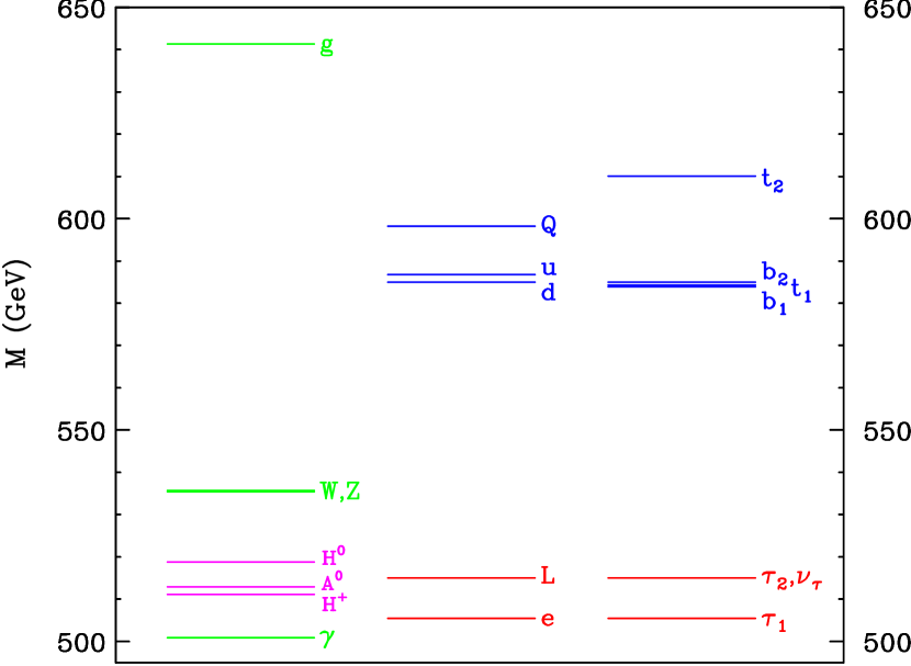
Figure 17: One-loop corrected mass spectrum of the first KK level for $R^{-1}=500$ GeV, $\Lambda R=20$ and $m_{h}=120$ GeV. The states $t_{1,2}$, $b_{1,2}$, and $\tau_{1,2}$ correspond to the mass eigenstates of the first KK excitations of the left- and right-handed SM fermions. (Fig. 1 from Ref. [62].)

for a compactification size relevant to upcoming collider experiments.

I should emphasize that there are several assumptions built into this radiatively-corrected spectrum. One is that the matching contributions to the brane-localized kinetic terms are assumed to be zero when evaluated at the cutoff scale. This leads to a finite correction that should be compared against a log-enhanced correction. However, since the log is relatively small, of order $\ln 30\sim 3.4$, the finite contribution could easily compete or dominate over this correction. Also, the spectrum assumes that there are no brane-localized quadratically-divergent contributions to the Higgs (mass)².

Nevertheless, it is intriguing that the spectrum is so qualitatively similar to a moderately degenerate supersymmetric spectrum. The spin of the KK excitations is of course equal to the spin of the corresponding SM (zero mode) field, whereas superpartners have spin that differ by $1/2$ from their SM counterparts. Unfortunately, measurements of the spin of newly discovered heavy particles at hadron colliders is not easy. This had led to suggestions that a KK spectrum could easily be mistaken for a degenerate supersymmetric spectrum [62].

Another similarity to supersymmetry is that UED possesses an auxiliary discrete symmetry that (if exact) forces pair production of the lightest level-one KK excitations and prevents the lightest level-one KK excitation from decaying into SM particles. The latter property implies that a stable particle exists in the spectrum, potentially a dark matter candidate.

If the spectrum of the level-one KK excitations follows precisely that of Eqs. (175), then the lightest KK particle is the KK photon. Saying “KK photon” is somewhat misleading, however, since the neutral gauge boson mass matrix in the ($B^{(n)}$, $W^{3(n)}$) basis

$$\left(\begin{array}[]{cc}\frac{n^{2}}{R^{2}}+\delta m^{2}_{B^{(n)}}+\frac{1}{4}g^{\prime 2}v^{2}&\frac{1}{4}g^{\prime}gv^{2}\\ \frac{1}{4}g^{\prime}gv^{2}&\frac{n^{2}}{R^{2}}+\delta m^{2}_{W^{(n)}}+\frac{1}{4}g^{2}v^{2}\end{array}\right)$$ (176)

depends on both the tree-level contributions (proportional to $v^{2}$) and the radiative corrections. The effective mixing angle, $\sin^{2}\theta_{W}^{(n)}$ for the $n^{\rm th}$ mode is much smaller than the Weinberg angle, shown in Fig. 18.

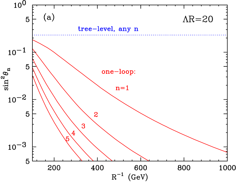
Figure 18: The effective Weinberg angle $\theta^{(n)}$ that determines the gauge content of the lightest level-$n$ KK mode, $\gamma^{(n)}=\cos\theta^{(n)}B^{(n)}-\sin\theta^{(n)}W^{3(n)}$. (Fig. 5 from Ref. [61].)

Clearly, for $1/R\gtrsim 500$ GeV combined with $\Lambda R\sim 20$, $\gamma^{(1)}\simeq B^{(1)}$ to within a percent, and so for all subsequent purposes we can consider them equivalent. From now on I’ll just use $B^{(1)}$ to refer to the lightest level-one KK excitation of the neutral gauge bosons.

4.9 UED Dark Matter

It is amusing that $B^{(1)}$ happens to be the candidate for dark matter in UED models. The close analogy with supersymmetry would seem to continue here, since the supersymmetric partner to the hypercharge gauge boson, the Bino ($\tilde{B}$), is the typical candidate for supersymmetric dark matter. But, this is where the similarity ends.

In supersymmetry, Bino annihilation typically proceeds through sfermion exchange, shown in Fig. 19(a). Since the Binos

Figure 19: Relevant annihilation and scattering processes for (a) supersymmetry and (b),(c) UED. The supersymmetric annihilation diagram (a) is $s$-wave suppressed by a factor $m_{f}^{2}/m_{B^{(1)}}$, whereas the UED diagram (b) is unsuppressed. Observable annihilation in the Sun occurs through diagram (b) with $f=\nu$. Annihilation in the galactic neighborhood to positrons occurs through diagram (b) with $f=\ell$. Scattering off nuclei occurs via diagram (c) with $f=q$, suitably “dressed” into a proton or neutron.

are Majorana fermions, Fermi statistics requires that they have their spins oppositely directed when prepared in an initial $s$-wave. This means that a chirality flip of the fermions is required, and thus a mass insertion in the diagram. This causes the cross section to be suppressed by a factor $m_{f}^{2}/m_{\tilde{B}}^{2}$.

In UED, $B^{(1)}$ annihilation also proceeds through KK fermion annihilation shown in Fig. 19(b), but because the incoming states are bosons, there is no $s$-wave suppression. This means that the mass range for $B^{(1)}$ to make up the dark matter of the Universe is significantly higher than the range of Bino masses for supersymmetric dark matter. We can estimate the thermally-averaged annihilation cross section by assuming that only diagrams of type (b) shown in Fig. 19 are present. Given the KK spectrum above, Eqs. (175), the radiative correction to level-one KK fermions is typically at the few to tens of percent level. A reasonable approximation is to assume that the mass of the exchanged KK particle $f^{(1)}$ is roughly degenerate with $B^{(1)}$. The cross section is then simply $1/m_{B^{(1)}}^{2}$ times the coupling factors, which are just $g_{1}^{4}\sum_{i}(Y_{f}^{i})^{4}$. The final result is

$$\langle\sigma v\rangle=\frac{95g_{1}^{4}}{324\pi m_{B^{(1)}}^{2}}$$ (177)

where this cross section with numerical factors was worked out in Ref. [65]. If you take a rough estimate of the relic density given in Kolb and Turner [75]

$$\Omega h^{2}\sim\frac{0.77\times 10^{-37}\;{\rm cm}^{2}}{\langle\sigma v\rangle}$$ (178)

and then plug in the thermally-averaged cross section above, one obtains

$$\Omega h^{2}\sim 0.1\left(\frac{m_{B^{(1)}}}{1\;{\rm TeV}}\right)^{2}$$ (179)

which is accurate to within about 15% of the numerical results given in Ref. [65]. A plot of the relic density is shown in Fig. 20, along with several additional

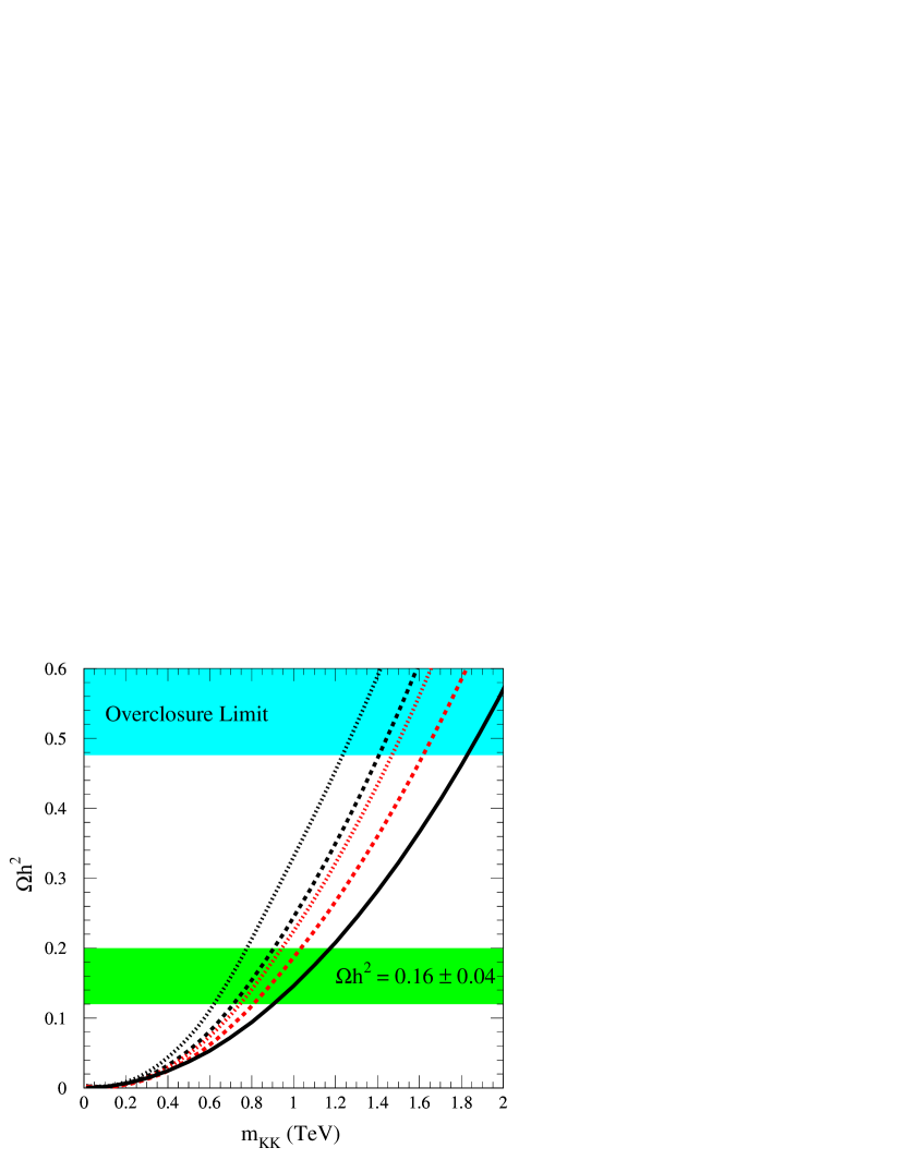
Figure 20: Prediction for $\Omega_{B^{(1)}}h^{2}$. The solid line is the case for $B^{(1)}$ alone, and the dashed and dotted lines correspond to the case in which there are one (three) flavors of nearly degenerate $e_{R}^{(1)}$. For each case, the black curves (upper of each pair) denote the case where the fractional mass difference between the RH KK lepton and $B^{(1)}$ is 1%, while the red curves (lower of each pair) correspond to 5%. Note that the “favorable range” of $\Omega h^{2}$ for dark matter is now out-of-date; current cosmological data suggest $\Omega h^{2}\sim 0.1$, just below the bottom of the shaded band. (Fig. 3 from Ref. [65].)

curves that represent including coannihilation with one to three generations of the level-one KK excitations of the right-handed leptons.

An interesting outcome of the analysis of Ref. [65] is that coannihilation with light KK leptons causes an increase in the effective annihilation cross section and thus a decrease in the mass range of the KK particle. This happens because the additional KK particles, when close enough in mass to $B^{(1)}$, have small annihilation and coannihilation cross sections, freeze out later, causing them to act as additional components to dark matter. These right-handed (RH) KK leptons decay into $B^{(1)}$ after their mutual interactions are too slow compared with the expansion rate, and thus they decay into $B^{(1)}$, boosting the $B^{(1)}$ relic density, or equivalently lowering the mass range of $B^{(1)}$ when the relic density is held fixed.

This result, however, is unique to right-handed KK leptons. As shown by two groups Refs. [77, 78], coannihilation with left-handed KK leptons, KK quarks, KK gluons, etc., all have cross sections that are larger than $B^{(1)}$ annihilation, causing the total effective cross section to go up. Holding the relic density fixed, this implies the mass range of $B^{(1)}$ must also increase. If the KK quarks and KK gluon are below about $1.1$ times the mass of $B^{(1)}$, these coannihilation effects can cause the mass range for $B^{(1)}$ to go up to the few TeV range. On face value, such a small separation between the mass of $B^{(1)}$ and the strongly interacting level-one KK particles is not expected from the radiative corrections to the masses of the first KK level computed in [61]. However, if the cutoff scale is not much larger than the compactification scale, and thus matching corrections are comparable in size while opposite in sign to compensate, the level-one KK spectrum could be much more degenerate.

UED dark matter can be detected by the usual methods, namely direct detection by scattering off nuclei, as well as indirect detection through annihilation in the Sun to neutrinos or annihilation in our galactic neighborhood to positrons.

4.10 Direct Detection of UED Dark Matter

First consider the direct detection of $B^{(1)}$ dark matter. Dark matter particles are currently non-relativistic, with velocity $v\sim 10^{-3}$. For weak scale dark matter, the recoil energy from scattering off nuclei is far less than for scattering off electrons, and thus one need only consider elastic scattering off nucleons and nuclei.

At the quark level, $B^{(1)}$ scattering goes through KK quarks, such as shown in Fig. 19(c). The amplitudes and cross sections for the quark level processes are easy to calculate, but then these processes must be convoluted with structure functions for nucleons and nuclei. The interactions divide into spin-dependent and spin-independent parts [79]. Higgs exchange contributes to scalar couplings, while KK quark exchange contributes to both.

In Refs. [80, 81] both spin-independent and spin-dependent cross sections were calculated and are shown in Fig. 21. This figure assumes all level-one KK quarks are

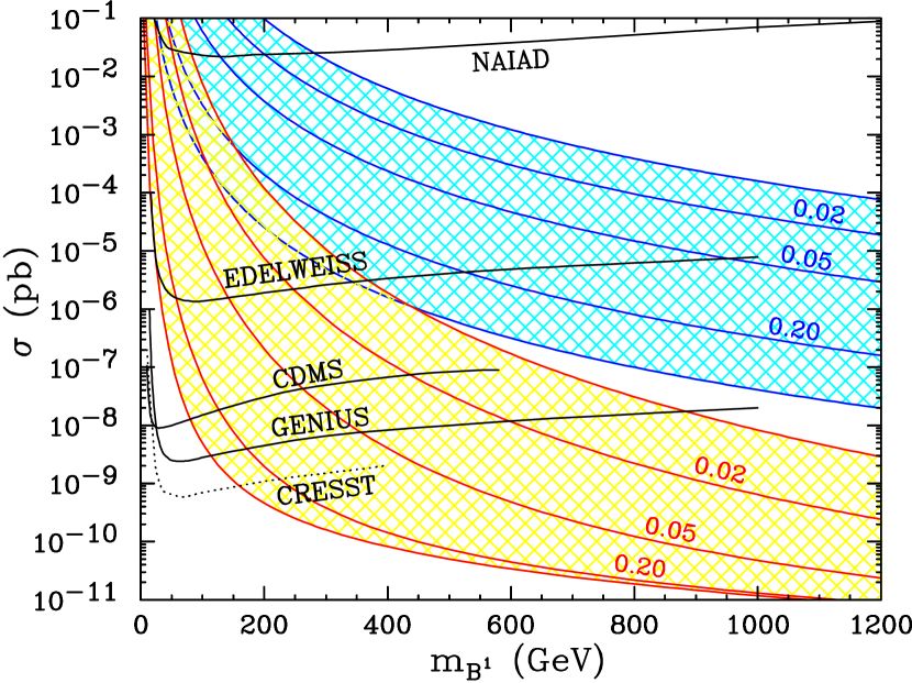
Figure 21: Predicted spin-dependent proton cross sections (dark-shaded, blue), along with the projected sensitivity of a 100 kg NAIAD array; and predicted spin-independent proton cross sections (light-shaded, red), along with the current EDELWEISS sensitivity, and projected sensitivities of CDMS, GENIUS, and CRESST. The predictions are for $m_{h}=120$ GeV and $0.01\leq r=(m_{q^{1}}-m_{B^{(1)}})/m_{B^{(1)}}\leq 0.5$, with contours for specific intermediate $r$ labeled. (Fig. 1 from Ref. [80].)

degenerate with mass $m_{q^{(1)}}$ that is different from $m_{B^{(1)}}$. Projected sensitivities of near future experiments are also shown in Fig. 21. For scattering off individual nucleons, scalar cross sections are suppressed relative to spin-dependent ones by $\sim m_{p}/m_{B^{(1)}}$. However, this effect is compensated in large nuclei where spin-independent rates are enhanced by $\sim A^{2}$ ($A$ is the nuclei mass number). In the case of bosonic UED dark matter, the latter effect dominates, and the spin-independent experiments have the best prospects for detection with sensitivity to $m_{B^{(1)}}$ far above current limits.

4.11 Indirect Detection of UED Dark Matter

Figure 22: The number of events per year in a detector with effective area equal to one square kilometer. Contours are shown for $r_{q^{(1)}_{R}}=0.1$, $0.2$, and $0.3$. The $r_{q^{(1)}_{R}}=0.3$ is shown merely for comparison, since this mass ratio is larger than would be expected from the one-loop radiative correction calculations of the KK mode masses. The relic density of the $B^{(1)}$’s lies within the range $\Omega_{B^{(1)}}h^{2}=0.16\pm 0.04$ for the solid sections of each line. Matching to the WMAP data, in which $\Omega_{B^{(1)}}h^{2}\sim 0.1$ is preferred, corresponds roughly to the left-hand side dash-to-solid transition for each curve. (Fig. 2 from [82].)

Weakly interacting dark matter particles are expected to become gravitationally trapped in large bodies, such as the Sun, and annihilate into neutrinos or other particles that decay into neutrinos. The calculation of the flux of neutrinos from particle dark matter annihilation in the Sun has been explored in some detail, particularly the case of neutralino dark matter (for reviews, see Refs. [18, 20]). The basic idea is to begin with the relatively well-known local dark matter density from the galactic rotation data, compute the interaction cross section of the particle dark matter with nuclei in the Sun, compare the capture rate with the annihilation rate to determine if these processes are in equilibrium, and then compute the flux of neutrinos that result from this rate capture and annihilation. There is a huge detector at the south pole that has instrumented a large area of antarctic ice by stringing detectors down deep holes. The first version of this experiment had an effective area of $0.1\;{\rm km}^{2}$ (called AMANDA) that is now in progress towards expansion to $1\;{\rm km}^{2}$ (called IceCube).

The calculation of the annihilation rate in the Sun involves similar scattering processes to what we found for direct detection, except that now the dominant process is simply scattering off protons. The new ingredient is to determine when the capture rate equilibrates with the annihilation rate, which is determined by the mass of the (core of the) Sun, the dark matter density and (relative) velocity, as well as the microscopic scattering cross section. Since the particle dark matter candidate in UED is rather heavy, it is not surprising that the elastic scattering is not particularly large, and a detailed calculation [82] shows that $B^{(1)}$ dark matter just barely comes into equilibrium after 4.5 billion years. This gives the maximal neutrino signal emitted from the Sun.

The actual outgoing flux depends on the annihilation fraction directly into neutrinos, as well as indirectly through decays. Muon neutrinos are the main actors, since at the energies relevant to $B^{(1)}$ annihilation, neutrino telescopes only observe muon tracks generated in charged-current interactions. In Ref. [82] the heavier level-one KK modes were approximated to have about the same mass, but this mass was taken to be slightly larger than $m_{B^{(1)}}$ by a fraction

$$r_{f^{(1)}}\equiv\frac{m_{f^{(1)}}-m_{B^{(1)}}}{m_{B^{(1)}}}\;,$$ (180)

typically about $0.1$–$0.2$ given the spectrum from Eqs. (175). Using the neutrino energy spectrum, the event rate expected at an existing or future neutrino telescope can be calculated. This is shown in Fig. 22 for a detector with an effective area of $1\;{\rm km}^{2}$. Combining the spectrum determined by the one-loop radiative corrections with a relic density appropriate for dark matter, the expectation is to get between a few to tens of events per year at the IceCube detector.

Finally, there are speculations that UED dark matter annihilation in the galactic halo might account for the positron excess, see Ref. [83] for details.

5 Conclusions

In these lectures I have showed how the phenomenology of extra dimensions is very rich, should Nature choose to follow one or more of the ideas discussed in this review. I have tried to give a overview of what I perceive to be the main characteristic signals of the specific extra dimensional models that I discussed. Nevertheless, there are several related models and a host of other aspects to extra dimensions that I did not have the time or space to review. This remains a very active field of investigation with new ideas continually being developed.

How likely is any given extra dimensional proposal? This is not a question that has any scientific answer, even though physicists try hard to quantify their qualitative instincts. This much can be said with relative certainty: In all cases the cutoff scale of the Standard Model is drastically lowered from the Planck scale to near the TeV scale. Since the lore of quantum gravity is that all global symmetries are broken by Planck scale effects, naturalness suggests cutoff-scale suppressed higher dimensional operators should appear at the 1/TeV level with order one coefficients. If this were true, all of these models would be ruled out immediately by $B$ and $L$ violating operators, operators leading to FCNC, and operators modifying precision electroweak observables. As model builders, we must conclude that either the cutoff scale (i.e., the quantum gravity scale) is larger or there are mechanisms to suppress or eliminate these dangerous effects. Some of these remarkably creative mechanisms were discussed or referenced in the preceding sections. As phenomenologists, however, we are blissfully free to assume that these operators are suppressed by an unspecified mechanism or simply tuned to be small, and then we have the opportunity to probe the physics of these scenarios directly in colliders and indirectly in all sorts of ways from astrophysics to table-top experiments.

During the lectures, I repeatedly emphasized that while extra dimensions are interesting in themselves, the real take home lesson is to understand how to turn “great model A” into “predictions 1,2,3” and compare with “experiments X,Y,Z”. Extra dimensions provide a fascinating and exciting set of models to illustrate precisely this important exercise. As we approach the next energy frontier with the LHC and future experiments, I hope these lectures instill some of the techniques to turn new physics ideas into a testable theory. Good luck developing your own great ideas and turning them into calculable phenomenology!

References

- [1] N. Arkani-Hamed, S. Dimopoulos and G. R. Dvali, Phys. Lett. B 429, 263 (1998) [arXiv:hep-ph/9803315].
- [2] L. Randall and R. Sundrum, Phys. Rev. Lett. 83, 3370 (1999) [arXiv:hep-ph/9905221].
- [3] T. Appelquist, H. C. Cheng and B. A. Dobrescu, Phys. Rev. D 64, 035002 (2001) [arXiv:hep-ph/0012100].
- [4] T. Kaluza, Sitzungsber. Preuss. Akad. Wiss. Berlin (Math. Phys. ) 1921, 966 (1921); O. Klein, Z. Phys. 37, 895 (1926) [Surveys High Energ. Phys. 5, 241 (1986)].
- [5] B. Zwiebach, “A first course in string theory,” Cambridge University Press (2004).
- [6] R. Sundrum, arXiv:hep-th/0508134.
- [7] C. Csaki, J. Hubisz and P. Meade, arXiv:hep-ph/0510275.
- [8] N. Arkani-Hamed, A. G. Cohen and H. Georgi, Phys. Rev. Lett. 86, 4757 (2001) [arXiv:hep-th/0104005].
- [9] C. T. Hill, S. Pokorski and J. Wang, Phys. Rev. D 64, 105005 (2001) [arXiv:hep-th/0104035].
- [10] N. Arkani-Hamed, H. Georgi and M. D. Schwartz, Annals Phys. 305, 96 (2003) [arXiv:hep-th/0210184]; N. Arkani-Hamed and M. D. Schwartz, Phys. Rev. D 69, 104001 (2004) [arXiv:hep-th/0302110]; M. D. Schwartz, Phys. Rev. D 68, 024029 (2003) [arXiv:hep-th/0303114].
- [11] N. Arkani-Hamed, S. Dimopoulos and G. R. Dvali, Phys. Rev. D 59, 086004 (1999) [arXiv:hep-ph/9807344].
- [12] E. Witten, Nucl. Phys. B 443, 85 (1995) [arXiv:hep-th/9503124]; P. Horava and E. Witten, Nucl. Phys. B 460, 506 (1996) [arXiv:hep-th/9510209]; J. D. Lykken, Phys. Rev. D 54, 3693 (1996) [arXiv:hep-th/9603133]; T. Banks and M. Dine, Nucl. Phys. B 479, 173 (1996) [arXiv:hep-th/9605136]. I. Antoniadis, N. Arkani-Hamed, S. Dimopoulos and G. R. Dvali, Phys. Lett. B 436, 257 (1998) [arXiv:hep-ph/9804398].
- [13] See for example I. Antoniadis, Phys. Lett. B 246, 377 (1990); I. Antoniadis and K. Benakli, Phys. Lett. B 326, 69 (1994) [arXiv:hep-th/9310151]; K. R. Dienes, E. Dudas and T. Gherghetta, Phys. Lett. B 436, 55 (1998) [arXiv:hep-ph/9803466]; K. R. Dienes, E. Dudas and T. Gherghetta, Nucl. Phys. B 537, 47 (1999) [arXiv:hep-ph/9806292].
- [14] T. Han, G. D. Kribs and B. McElrath, Phys. Rev. Lett. 90, 031601 (2003) [arXiv:hep-ph/0207003].
- [15] E. G. Adelberger, B. R. Heckel and A. E. Nelson, Ann. Rev. Nucl. Part. Sci. 53, 77 (2003) [arXiv:hep-ph/0307284].
- [16] C. D. Hoyle, D. J. Kapner, B. R. Heckel, E. G. Adelberger, J. H. Gundlach, U. Schmidt and H. E. Swanson, Phys. Rev. D 70, 042004 (2004) [arXiv:hep-ph/0405262].
- [17] L. J. Hall, Prepared for 30th International Conference on High-Energy Physics (ICHEP 2000), Osaka, Japan, 27 Jul - 2 Aug 2000
- [18] G. Jungman, M. Kamionkowski and K. Griest, Phys. Rept. 267, 195 (1996) [arXiv:hep-ph/9506380].
- [19] K. A. Olive, arXiv:astro-ph/0301505.
- [20] G. Bertone, D. Hooper and J. Silk, Phys. Rept. 405, 279 (2005) [arXiv:hep-ph/0404175].
- [21] G. F. Giudice, R. Rattazzi and J. D. Wells, Nucl. Phys. B 544, 3 (1999) [arXiv:hep-ph/9811291].
- [22] H. van Dam and M. J. G. Veltman, Nucl. Phys. B 22, 397 (1970); V. I. Zakharov, JETP Lett. 12, 312 (1970).
- [23] N. Arkani-Hamed, S. Dimopoulos and J. March-Russell, Phys. Rev. D 63, 064020 (2001) [arXiv:hep-th/9809124].
- [24] T. Banks, M. Dine and A. E. Nelson, JHEP 9906, 014 (1999) [arXiv:hep-th/9903019].
- [25] C. Csaki, M. Graesser and J. Terning, Phys. Lett. B 456, 16 (1999) [arXiv:hep-ph/9903319].
- [26] E. A. Mirabelli, M. Perelstein and M. E. Peskin, Phys. Rev. Lett. 82, 2236 (1999) [arXiv:hep-ph/9811337].
- [27] T. Han, J. D. Lykken and R. J. Zhang, Phys. Rev. D 59, 105006 (1999) [arXiv:hep-ph/9811350].
- [28] J. L. Hewett, Phys. Rev. Lett. 82, 4765 (1999) [arXiv:hep-ph/9811356].
- [29] S. Eidelman et al. [Particle Data Group], Phys. Lett. B 592, 1 (2004).
- [30] G. G. Raffelt, Ann. Rev. Nucl. Part. Sci. 49, 163 (1999) [arXiv:hep-ph/9903472].
- [31] S. Cullen and M. Perelstein, Phys. Rev. Lett. 83, 268 (1999) [arXiv:hep-ph/9903422].
- [32] N. Arkani-Hamed, S. Dimopoulos, N. Kaloper and J. March-Russell, Nucl. Phys. B 567, 189 (2000) [arXiv:hep-ph/9903224].
- [33] A. Burrows et al., arXiv:astro-ph/9709278.
- [34] L. J. Hall and D. R. Smith, Phys. Rev. D 60, 085008 (1999) [arXiv:hep-ph/9904267].
- [35] K. Agashe, A. Delgado, M. J. May and R. Sundrum, JHEP 0308, 050 (2003) [arXiv:hep-ph/0308036]; K. Agashe, R. Contino and A. Pomarol, Nucl. Phys. B 719, 165 (2005) [arXiv:hep-ph/0412089].
- [36] C. Csaki, C. Grojean, L. Pilo and J. Terning, Phys. Rev. Lett. 92, 101802 (2004) [arXiv:hep-ph/0308038].
- [37] N. J. Nunes and M. Peloso, Phys. Lett. B 623, 147 (2005) [arXiv:hep-th/0506039].
- [38] S. B. Giddings, S. Kachru and J. Polchinski, Phys. Rev. D 66, 106006 (2002) [arXiv:hep-th/0105097].
- [39] L. Randall and R. Sundrum, Phys. Rev. Lett. 83, 4690 (1999) [arXiv:hep-th/9906064].
- [40] C. Csaki, arXiv:hep-ph/0404096.
- [41] H. Davoudiasl, J. L. Hewett and T. G. Rizzo, Phys. Rev. Lett. 84, 2080 (2000) [arXiv:hep-ph/9909255].
- [42] W. D. Goldberger and M. B. Wise, Phys. Rev. Lett. 83, 4922 (1999) [arXiv:hep-ph/9907447].
- [43] C. Csaki, M. L. Graesser and G. D. Kribs, Phys. Rev. D 63, 065002 (2001) [arXiv:hep-th/0008151].
- [44] T. Tanaka and X. Montes, Nucl. Phys. B 582, 259 (2000) [arXiv:hep-th/0001092].
- [45] C. Charmousis, R. Gregory and V. A. Rubakov, Phys. Rev. D 62, 067505 (2000) [arXiv:hep-th/9912160].
- [46] O. DeWolfe, D. Z. Freedman, S. S. Gubser and A. Karch, Phys. Rev. D 62, 046008 (2000) [arXiv:hep-th/9909134].
- [47] C. Csaki, M. Graesser, L. Randall and J. Terning, Phys. Rev. D 62, 045015 (2000) [arXiv:hep-ph/9911406].
- [48] W. D. Goldberger and M. B. Wise, Phys. Lett. B 475, 275 (2000) [arXiv:hep-ph/9911457].
- [49] H. L. Verlinde, Nucl. Phys. B 580, 264 (2000) [arXiv:hep-th/9906182].
- [50] N. Arkani-Hamed, M. Porrati and L. Randall, JHEP 0108, 017 (2001) [arXiv:hep-th/0012148].
- [51] R. Rattazzi and A. Zaffaroni, JHEP 0104, 021 (2001) [arXiv:hep-th/0012248].
- [52] I. R. Klebanov, arXiv:hep-th/0009139; J. M. Maldacena, arXiv:hep-th/0309246.
- [53] K. m. Cheung, Phys. Rev. D 63, 056007 (2001) [arXiv:hep-ph/0009232].
- [54] G. F. Giudice, R. Rattazzi and J. D. Wells, Nucl. Phys. B 595, 250 (2001) [arXiv:hep-ph/0002178].
- [55] M. Shiozawa et al. [Super-Kamiokande Collaboration], Phys. Rev. Lett. 81, 3319 (1998) [arXiv:hep-ex/9806014].
- [56] S. Nussinov and R. Shrock, Phys. Rev. Lett. 88, 171601 (2002) [arXiv:hep-ph/0112337].
- [57] N. Arkani-Hamed and M. Schmaltz, Phys. Rev. D 61, 033005 (2000) [arXiv:hep-ph/9903417].
- [58] H. Davoudiasl, R. Kitano, G. D. Kribs and H. Murayama, Phys. Rev. D 71, 113004 (2005) [arXiv:hep-ph/0502176].
- [59] T. Appelquist, B. A. Dobrescu, E. Ponton and H. U. Yee, Phys. Rev. Lett. 87, 181802 (2001) [arXiv:hep-ph/0107056].
- [60] B. A. Dobrescu and E. Poppitz, Phys. Rev. Lett. 87, 031801 (2001) [arXiv:hep-ph/0102010].
- [61] H. C. Cheng, K. T. Matchev and M. Schmaltz, Phys. Rev. D 66, 036005 (2002) [arXiv:hep-ph/0204342].
- [62] H. C. Cheng, K. T. Matchev and M. Schmaltz, Phys. Rev. D 66, 056006 (2002) [arXiv:hep-ph/0205314].
- [63] M. Battaglia, A. Datta, A. De Roeck, K. Kong and K. T. Matchev, JHEP 0507, 033 (2005) [arXiv:hep-ph/0502041].
- [64] A. Datta, K. Kong and K. T. Matchev, Phys. Rev. D 72, 096006 (2005) [Erratum-ibid. D 72, 119901 (2005)] [arXiv:hep-ph/0509246].
- [65] G. Servant and T. M. P. Tait, Nucl. Phys. B 650, 391 (2003) [arXiv:hep-ph/0206071].
- [66] J. D. Lykken, arXiv:hep-th/9612114.
- [67] Z. Chacko, M. A. Luty and E. Ponton, JHEP 0007, 036 (2000) [arXiv:hep-ph/9909248].
- [68] L. Alvarez-Gaume and E. Witten, Nucl. Phys. B 234, 269 (1984).
- [69] G. D. Kribs, Phys. Rev. D 69, 111701 (2004) [arXiv:hep-ph/0304256].
- [70] E. Witten, Phys. Lett. B 117, 324 (1982).
- [71] H. Georgi, A. K. Grant and G. Hailu, Phys. Lett. B 506, 207 (2001) [arXiv:hep-ph/0012379].
- [72] M. E. Peskin and T. Takeuchi, Phys. Rev. D 46, 381 (1992).
- [73] T. G. Rizzo and J. D. Wells, Phys. Rev. D 61, 016007 (2000) [arXiv:hep-ph/9906234].
- [74] R. S. Chivukula, D. A. Dicus, H. J. He and S. Nandi, Phys. Lett. B 562, 109 (2003) [arXiv:hep-ph/0302263].
- [75] E. W. Kolb and M. S. Turner, “The Early Universe,” Addison-Wesley (1990).
- [76] K. Griest and D. Seckel, Phys. Rev. D 43, 3191 (1991).
- [77] F. Burnell and G. D. Kribs, Phys. Rev. D 73, 015001 (2006) [arXiv:hep-ph/0509118].
- [78] K. Kong and K. T. Matchev, arXiv:hep-ph/0509119.
- [79] M. W. Goodman and E. Witten, Phys. Rev. D 31, 3059 (1985).
- [80] H. C. Cheng, J. L. Feng and K. T. Matchev, Phys. Rev. Lett. 89, 211301 (2002) [arXiv:hep-ph/0207125].
- [81] G. Servant and T. M. P. Tait, New J. Phys. 4, 99 (2002) [arXiv:hep-ph/0209262].
- [82] D. Hooper and G. D. Kribs, Phys. Rev. D 67, 055003 (2003) [arXiv:hep-ph/0208261].
- [83] D. Hooper and G. D. Kribs, Phys. Rev. D 70, 115004 (2004) [arXiv:hep-ph/0406026].